A Hybrid Feature Selection Framework Using Improved Sine Cosine Algorithm with Metaheuristic Techniques

Abstract

Feature selection is the procedure of extracting the optimal subset of features from an elementary feature set, to reduce the dimensionality of the data. It is an important part of improving the classification accuracy of classification algorithms for big data. Hybrid metaheuristics is one of the most popular methods for dealing with optimization issues. This article proposes a novel feature selection technique called MetaSCA, derived from the standard sine cosine algorithm (SCA). Founded on the SCA, the golden sine section coefficient is added, to diminish the search area for feature selection. In addition, a multi-level adjustment factor strategy is adopted to obtain an equilibrium between exploration and exploitation. The performance of MetaSCA was assessed using the following evaluation indicators: average fitness, worst fitness, optimal fitness, classification accuracy, average proportion of optimal feature subsets, feature selection time, and standard deviation. The performance was measured on the UCI data set and then compared with three algorithms: the sine cosine algorithm (SCA), particle swarm optimization (PSO), and whale optimization algorithm (WOA). It was demonstrated by the simulation data results that the MetaSCA technique had the best accuracy and optimal feature subset in feature selection on the UCI data sets, in most of the cases.

1. Introduction

With the explosive growth of data resources in modern society, data mining not only has a crucial effect on various industries, but has also become the key to the core competitiveness of various industries [1,2,3]. Data mining is the operation of extracting hidden patterns from extensive data in conditions of incomplete, noisy, and random row data, which is helpful for people to make decisions [4,5,6]. However, due to the huge amount of data and the existence of redundant data, it is difficult to obtain the information directly from big data that can help in decision making. Based on the above statements, we can see that data pre-processing has a meaningful impact on the success of big data mining [7,8,9]. In addition, feature selection is a key step in data preprocessing. [10,11,12].

For deterministic datasets, since the presence of irrelevant features does not affect the accuracy of the classification algorithm, training the classifier using the primary feature set will increase the computational overhead of the classifier and will not enhance the classification performance of the classifier [13,14,15]. Therefore, feature selection enables reducing the feature dimensionality of the original dataset. [16,17]. This can not only improve the efficiency of classifier, but also save computational resources [18,19,20].

There are various main models for feature selection [21,22]: the filtering model, embedding model, and packing model [23]. The main idea of the filtering model is to score each feature using a proxy measurement, then obtain the importance ranking sequence of all features, and finally choose the optimal feature subset among the sort sequence, according to the set threshold of the number of features. In addition, the filtering model first chooses the optimal subset of features, and then trains the learner. Common proxy metrics include the chi-square test, information gain, correlation coefficient, and so on [24,25,26]. The main idea of the embedded model is to complete the feature selection operation in conjunction with the learner fitting operation, to obtain the feature subset with higher classification accuracy [27,28]. The package model treats the optimization problem for a subset of features as an optimization issue [29,30]. The package model first generates several different feature subsets, then calculates the fitness of all feature subsets by using the adaptation function, and, finally, finds the feature subset with the highest adaptation value, as the best feature subset. There are many common metaheuristic optimization algorithms that can address this problem [31], examples include particle swarm optimization (PSO) [32], genetic algorithm (GA) [33], and sine cosine algorithm (SCA) [34].

Meta-heuristic optimization is a common approach to solving global optimization issues. Unlike the traditional optimization techniques, such as simulated annealing with gradient descent, the metaheuristic algorithm is a flexible optimization method that can ignore gradient variations. The SCA is an optimization that is subject to population intelligence among metaheuristic algorithms [35]. However, similarly to the different population intelligence-based algorithms, the optimization strategy of the SCA is prone to local optimization and unbalanced exploration [36], which leads to the difficulty of finding the optimal subset in feature selection using the SCA. For the purpose of settling the above problem, this article puts forward an improved SCA (MetaSCA) feature selection model. The principal contributions of the work are listed below.

(1)

We propose a hybrid feature selection framework, using an improved SCA with metaheuristic techniques to reduce the dimensionality of data in the face of the curse of dimensionality due to a large number of features in a dataset.

(2)

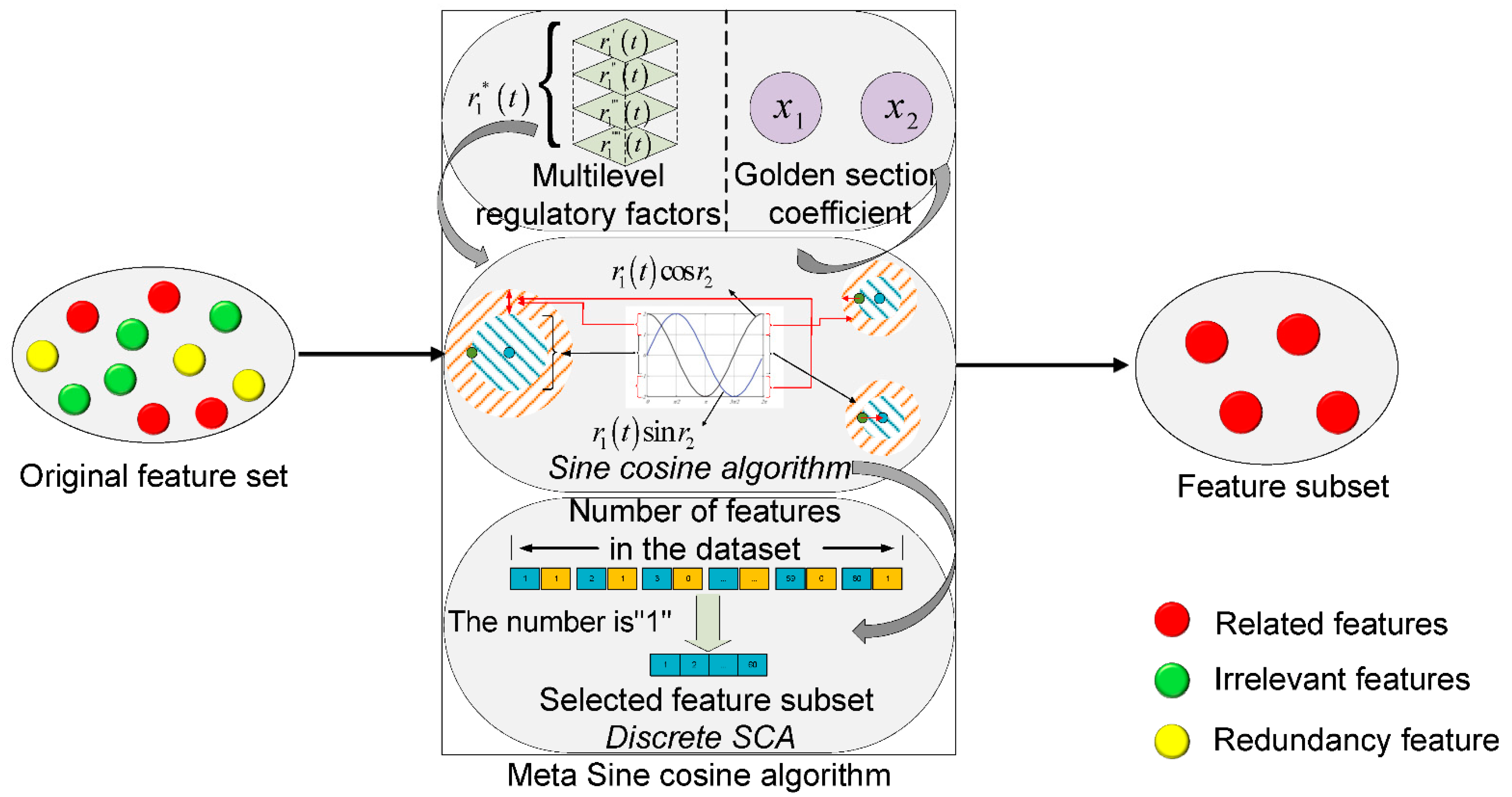
We analyze the optimization performance of the standard SCA algorithm and point out that the algorithm has difficulty in selecting the best feature subset during feature selection. An improved SCA (MetaSCA), based on the multilevel regulatory factor strategy and the golden section coefficient strategy, is proposed to enhance the superiority-seeking effect of the SCA and implemented for the solution of the optimal feature subset.

(3)

We tested the method with several datasets, to explore the performance of the method in feature selection. From the simulation results, we can see that the MetaSCA technique achieved good results in seeking the best feature subset.

The remainder of the article is organized as follows: Section 2 lists some related works in the literature. Section 3 describes the feature selection model and the problems to be solved in this article. Section 4 investigates the SCA and analyzes the optimization performance of the SCA. Based on this, the improved MetaSCA is proposed in this paper to solve the feature selection problem. Section 5 gives the simulation results of the MetaSCA in feature selection and discusses the potential of the scheme for feature selection. Section 6 gives the conclusions and features the work.

2. Related Works

In the past few years of investigation on big data classification and artificial intelligence, the number of features employed in applications has expanded from a few dozen to hundreds [37]. However, this excess of features will not only cause the curse of dimensionality, but also has a negative impact on the problems explored. Therefore, after obtaining a large number of data features, we need to select the relevant ones that are helpful to the problem from all the features. Feature selection is a method for achieving this goal [19,22,38]. Moreover, feature selection is broadly classified into filtering models, embedding models, and packing models. As one of the packing models, heuristic search is a method that uses heuristic information to continuously reduce the search space, which reduces the impact of excessive computation in finding the best feature subset in a high-dimensional feature area [39]. Therefore, metaheuristic search methods are combined with classifier models to acquire the best feature subset. Several metaheuristic models are given below that handle feature selection.

Two feature selection models founded on the whale optimization algorithm (WOA) have been proposed. The first model embedded the simulated annealing (SA) algorithm into the WOA, while the second one used the SA to refine the optimal solution obtained after each iteration of the WOA. [40]. Based on the WOA, two packing feature selection methods have been proposed. In the first method, the tournament and roulette selection mechanisms were used to replace the random operator in the conventional WOA. In the other method, the crossover and mutation operators were utilized to refine the WOA [41]. Feature selection founded on accelerated particle swarm optimization was created to enhance the accuracy of classification for high-dimensional data, when processing big data [32]. The method was applied to a set of high-dimensional data for feature selection and experimental evaluation. The simulation indicated that the lightweight feature selection acquired good results.

A new algorithm (UFSACO) contingent on the ant colony optimization algorithm was proposed and applied in feature selection [42]. The UFSACO did not use a learning algorithm and found the optimal feature subset through multiple iterations. This method had the advantages of low computational complexity and could solve the feature selection in high-dimensional data sets. The simulation results demonstrated the effectiveness of the UFSACO. An evolutionary crossover and mutation operator algorithm founded on the gravitational search algorithm (GSA) was presented in [43], to complete the task of feature selection. Simulation results showed the superiority of the algorithm in feature selection [43]. A fresh competitive binary gray wolf optimization method was put forward to accomplish the feature selection task in electromyography (EMG) signal classification. This method was compared with the binary gray wolf algorithm, the binary particle swarm optimization algorithm, and the GA. The simulation data illustrated that the method [44] not only had a better classification performance in using the selected optimal feature subset, but also had big advantages in feature reduction.

For the subset of feature selection, an enhanced Harris hawks optimization (IHHO) contingent on Harris hawks optimization (HHO) was put forward to select the optimal feature subset in a feature selection problem [45]. IHHO embedded the salp swarm algorithm (SSA) into conventional HHO, and compared this method with other feature selection methods. The simulation results indicated that using the optimal feature subset selected by IHHO to train the classifier could obtain a better classification. Integrated improved binary particle swarm optimization (iBPSO) with correlation-based feature selection (CFS) for cancer dataset classification resulted in a better performance accuracy of classification [46].

For feature selection, [47] an improved since cosine algorithm (ISCA) with elitism strategy and a new solution update mechanism was presented. The ISCA was compared for its performance in feature selection on data sets with the GA, PSO, and the SCA. Experimental results revealed that the algorithm advanced in [47] not only decreased the number of features, but also improved the classification performance. An improved Salp swarm optimizer, named ISSAFD, was proposed for feature selection in [48], based on the SCA and interrupt operator. The sinusoidal function was used to update the follower position in the SCA, to overcome the disadvantage of falling into the local optimum in the exploration stage. In addition, interruption strategies were added to strengthen the population diversity and to maintain a balance between global and local searches [48].

A novel hybrid optimization algorithm (SCAGA) based on the SCA and GA was advanced to handle the task of feature selection [49]. Evaluation of its fitness was made using the k-nearest neighbor algorithm for classification accuracy. The SCAGA was compared with the conventional SCA, ant colony optimization (ACO), and PSO on University of California Irvine (UCI) data sets for proficiency of feature selection. The experimental comparison showed that the SCAGA achieved the best performance in the test set. According to binary particle swarm optimization (BPSO) and the SCA, a hybrid optimization (HBPSOSCA) was proposed to select feature subsets with rich information from high-dimensional features for cluster analysis [50]. In [51], two binary metaheuristic algorithms based on the SCA called the SBSCA and the VBSCA for feature selection in medical data were presented. These algorithms generated each solution using two transfer functions. The simulation comparison results showed that the two methods proposed in [51] had a higher classification accuracy than the other four compared binary algorithms on the five medical datasets of the UCI repository.

In this study, an enhanced sine cosine algorithm (MetaSCA) is advanced for feature selection, using the multi-level regulatory factor strategy and the golden sine strategy. First, we transformed the continuous solution of the SCA into binary form, by mapping to determine feature selection and dropout. Then, the influence of the multi-level regulatory factor on the subset of features during SCA optimization was investigated with respect to diversity perspective. For the purpose of a more balanced exploration and exploitation in the optimization process, a multi-level regulatory factor strategy is proposed. Finally, the golden sine strategy is introduced to narrow down the feature solution space through golden partitioning and search only the space that yields good results.

3. System Model and Analysis

3.1. Feature Selection Model

An object often contains multiple features when dealing with classification problems. These characteristics fall into the following three broad categories.

• Related features: Such features help to complete the classification task and improve the fit of an algorithm.
• Irrelevant features: Irrelevant features that do not help to improve the fit of an algorithm, and which are not relevant to the task at hand.
• Redundancy feature: The improvement in classification performance brought by redundant features can also be obtained from other features.

Feature selection is the process of selecting all relevant features and discarding the redundant and irrelevant ones, to maximize the classification rate of the classifier and diminish the complexity of the original dataset when faced with all the features of the dataset. The feature selection framework put forward in this article is exhibited in Figure 1. The MetaSCA will be introduced in Section 4.

3.2. Problem Formulation

To decrease the difficulty of the learning task and increase the classification efficiency of the classification model, only relevant features need to be selected for training and fitting a classification algorithm. However, we cannot determine in advance which features are relevant. Therefore, we specify that the subset of features that contains fewer features, but that is better for the classification accuracy obtained by the classifier, is the optimal feature subset.

Assuming that the total quantity of features in the dataset is denoted as $m$, the original set of features is expressed as $F$ and the feature subset is represented as $F^{*}$. $F_i=1$ represents the selected feature in $F$. The problem of feature selection model can be formulated as follows:

$$\begin{array}{cc}Minimize& f\left(F^{*}\right)=\omega \times error\left(F^{*}\right)+\left(1-\omega \right)\times \frac{{{\displaystyle \sum }}_{i=1}^m{F}_i=1}{m}\\ Subject to& c1.F^{*}=\left\{F_i=1|\forall i\in m\right\}.\end{array}$$

(1)

where

$f\left(F^{*}\right)$—represents the fitness of feature subset $F^{*}$;

$error\left(F^{*}\right)$—stands for the error rate after classifying datasets using the feature subset;

${\displaystyle \sum }_{i=1}^m{F}_i=1$ represents the entire count of features in the feature subset $F^{*}$;

$\omega$ is a constant, which is used to determine the influence of $error\left(F^{*}\right)$ and $\frac{{{\displaystyle \sum }}_{i=1}^m{F}_i=1}{m}$ on the fitness function $f\left(F^{*}\right)$, respectively;

Let $c1$ be the feature subset that contains all features that are marked 1 in the original feature set.

4. Hybrid Framework with Metaheuristic Techniques

4.1. Sine Cosine Process

4.1.1. Conventional SCA Procedure

In this section, we give the optimization process of the conventional SCA.

Table 1. Symbols and their meanings.

Symbol	Definition
$X_t\left(i, j\right)$	Position of the i-th individual in iteration t
$X_t^{best}\left(i, j\right)$	Position of the best individual in the first t iterations
$r_1^{*}\left(t\right)$	Multilevel regulatory factor
$r_1\left(t\right)$	Regulatory factor
$r_2, r_3, r_4$	Random number with value range
$F_1$	Feature subset of the first generation
$F_t\left(i,j\right)$	i—th feature subset in the t—th iteration
$F_t^{best}\left(i,j\right)$	Optimal feature subset in the first t iterations
$E\left(F_t\right)$	Mathematical expectation of feature subset
D$\left(F_t\right)$	Variance of feature subset
I$\left(F_t\right)$	Diversity of feature subset
$pop$	Number of initially generated feature subsets
$dim$	Number of features in the original dataset
$f\left(x\right)$	Evaluation function
$T$	Maximum number of iterations
$a$	Lower boundary on the value of the feature subset
$b$	Upper boundary on the value of the feature subset
$x_1$	Golden section coefficient
$x_2$	Golden section coefficient

contains some symbols, and their corresponding meanings, that are used in this paper.

This algorithm has the advantages of simple parameters and clear results [35,52,53]. At the same time, the disadvantages of the SCA are obvious, such as the tendency to fall into the local optimum and a slow convergence rate [54]. The position update is mainly determined by the sine or cosine function, as shown in Equation (2).

$$X_{t+1}\left(i,j\right)=\left\{\begin{array}{c}{X}_t\left(i,j\right)+r_1\left(t\right)sin{r}_2\left|r_3{X}_t^{best}\left(i,j\right)-X_t\left(i,j\right)\right|, r_4<0.5\\ X_t\left(i,j\right)+r_1\left(t\right)cos{r}_2\left|r_3{X}_t^{best}\left(i,j\right)-X_t\left(i,j\right)\right|, r_4\ge 0.5\end{array}.\right.$$

(2)

where

$X_{t+1}\left(i,j\right)$—represents the position of individual $i$ in the $t+1$ round of dimension;

$j$, $X_t\left(i,j\right)$—represents the position of individual $i$ in the $t$ round of dimension $j$;

$X_t^{best}\left(i,j\right)$—represents the position of the global optimal solution in the previous $t$ rounds;

$r_1\left(t\right)$—represents the amplitude factor;

$r_1\left(t\right)=\alpha \left(1-\frac{t}{T}\right), \alpha =2, r_2\in \left[0, 2\pi \right], r_3\in \left[-2, 2\right], r_4\in \left[0, 1\right]$, and $r_2,r_3,r_4$ parameters are uniformly distributed random numbers.

The parameter $r_1$ determines the moving direction of $X_{t+1}\left(i,j\right)$; this direction could be either between the space of $X_t\left(i,j\right)$ and $X_t^{best}\left(i,j\right)$ or outside it. Moreover, $r_1$ also defines the exploration and exploitation of the update process of SCA. The $r_2$ defines how much $X_t\left(i,j\right)$ moves toward or away from $X_t^{best}\left(i,j\right)$. The $r_3$ parameter defines the degree of influence of the optimal solution $X_t^{best}\left(i,j\right)$ on the current solution $X_t\left(i,j\right)$. On the condition that $r3>1$ stochastically, the degree influence of X and Y should be weakened, otherwise they should be strengthened. The $r_4$ parameter controls the switch of the SCA, between the sine transform and cosine transform.

Figure 2 shows the conceptual schematic of the influence of the sine and cosine functions in the scope of $\left[-2, 2\right]$. The parameter $r_2$ determines whether the updated position of the solution appears between or outside the current solution and the optimal solution. When the value of $r_1\left(t\right)sin{r}_2$ or $r_1\left(t\right)cos{r}_2$ is in the scope of $\left[-2\right., \left.-1\right)\cup \left(1, \left.2\right]\right.$, the SCA conducts exploration. When the value of a is in the scope of $\left[-1, 1\right]$, the SCA conducts exploitation. Algorithm 1 shows the specific process of the SCA optimization.

Algorithm 1 Standard sine cosine algorithm

1. Input: Number of solution $pop$, dimension of solution $dim$, maximum number of iterations $T$, objective fitness function $f\left(x\right)$.

2. Initialize a solution set with $dim$ and $pop$ quality.

3. Calculate the fitness function value of each solution $X_t$ in the solution set according to $f\left(x\right)$, and find the solution $X_t^{best}$ with the smallest fitness value.

4.  Do (for each iteration)

5.    Update parameters $r_1\left(t\right),r_2,r_{3,} r_4$;

6.     Update the position of each solution $X_t$ in the solution set according to Formula 1;

7.    Calculate the fitness function value of each solution according to $f\left(x\right)$.

8.    Update current optimal solution $X_t^{best}$.

9.  While$(t<T$)

10. Output: Global optimal solution $X_t^{best}$ after iteration.

4.1.2. Analysis of the SCA in Feature Selection

In the initial stage of optimization using the SCA in feature selection, the SCA will randomly select multiple sets of features out of the original feature set to create $pop$ group feature subsets. Then, each feature subset is scored using the evaluation function, and the feature subset with the highest score is determined as the best feature subset. Next, the initialized feature subsets are perturbed according to Equation (2) to form new feature subsets with the number of $pop$. In addition, an evaluation function is used to assess the score of each new feature subset, and the feature subset with the best score is compared with the best feature subset in the previous round, to obtain the current best feature subset. The above process is repeated to obtain the best feature subset after the maximum round of iterations.

A key point in the SCA feature selection process is that the optimization strategy of the SCA affects the diversity of feature subsets. Next, we analyze the change of feature subset diversity during the process of the SCA updating the best feature subset. Assuming the formation of the initial feature subset is uniformly distributed, it has the probability density function of $F\sim u\left(a,b\right), f\left(F\right)=\frac{1}{b-a}, a\le F\le b$, where $F$ is the value of the feature subset, and $a$ and $b$ are the upper and lower boundaries of the range of values of the feature subset, respectively.

The expected value $E\left(F_1\right)$ and variance $D\left(F_1\right)$ of the first-generation feature subset are as follows:

$$\begin{gathered} E\left(F_1\right)={{\displaystyle \int }}_a^b\frac{F_1}{b-a}d{F}_1={\left.\frac{1}{2}\frac{F_1{}^2}{b-a}\right|}_a^b=\frac{b^2-a^2}{2\left(b-a\right)}=\frac{a+b}{2}, \\ E{\left(F_1\right)}^2={{\displaystyle \int }}_a^b\frac{F_1{}^2}{b-a}d{F}_1=\frac{1}{b-a}\frac{b^3-a^3}{3}=\frac{b^2+ab+a^2}{3}. \end{gathered}$$

(3)

$$D\left(F_1\right)=E{\left(F_1\right)}^2-{\left(E\left(F_1\right)\right)}^2=\frac{b^2+ab+a^2}{3}-{\left(\frac{a+b}{2}\right)}^2=\frac{{\left(b-a\right)}^2}{12}.$$

(4)

In this paper, the center of gravity is applied to portray the diversity of feature subsets. The diversity of $t$-generation feature subset $I\left(F_{t+1}\right)$ is defined as:

$$I\left(F_{t+1}\right)=\frac{1}{pop\times dim}{\displaystyle \sum }_{i=1}^{pop}{\displaystyle \sum }_{j=1}^{dim}{\left[F_{t+1}\left(i,j\right)-\frac{1}{N}\left({\displaystyle \sum }_{i=1}^N{F}_{t+1}\left(i,j\right)\right)\right]}^2.$$

$E\left(I\left(F_{t+1}\right)\right)$ is used to represent the expected value of $I\left(F_{t+1}\right)$:

$$E\left(I\left(F_{t+1}\right)\right)=\frac{1}{pop\times dim}{\displaystyle \sum }_{i=1}^{pop}{\displaystyle \sum }_{j=1}^{dim}E{\left[F_{t+1}\left(i,j\right)-\frac{1}{pop}\left({\displaystyle \sum }_{i=1}^{pop}{F}_{t+1}\left(i,j\right)\right)\right]}^2.$$

(5)

 Theorem  1. 

During the pursuit for the best feature subset by the SCA, the expectation value of the diversity of the feature subset in round$t+1$varies with the adjustment factor$r_1^2\left(t\right)$and the random number$r_3$.

 Proof of Theorem  1. 

First, ${\left[F_{t+1}\left(i,j\right)-\frac{1}{pop}\left({\displaystyle \sum }_{i=1}^{pop}{F}_{t+1}\left(i,j\right)\right)\right]}^2$ is expanded to obtain:

$$E{\left[F_{t+1}\left(i,j\right)-\frac{1}{pop}\left({\displaystyle \sum }_{i=1}^{pop}{F}_{t+1}\left(i,j\right)\right)\right]}^2=\left(\begin{array}{c}\underset{A}{\underbrace{E{\left[F_{t+1}\left(i,j\right)-E\left(F_{t+1}\left(i,j\right)\right)\right]}^2}-}\\ \underset{B}{\underbrace{2E\left(\left[F_{t+1}\left(i,j\right)-E\left(F_{t+1}\left(i,j\right)\right)\right]\times \left[\frac{1}{pop}{\displaystyle \sum }_{i=1}^{pop}{F}_{t+1}\left(i,j\right)-E\left(F_{t+1}\left(i,j\right)\right)\right]\right)}+}\\ \underset{C}{\underbrace{E{\left[\frac{1}{pop}{\displaystyle \sum }_{i=1}^{pop}{F}_{t+1}\left(i,j\right)-E\left(F_{t+1}\left(i,j\right)\right)\right]}^2}}\end{array}\right)$$

□

Second, expanded by Equation (5):

$$E\left(I\left(F_{t+1}\right)\right)==\frac{1}{pop\times dim}\times {\displaystyle \sum }_{i=1}^{pop}{\displaystyle \sum }_{j=1}^{dim}\left(\begin{array}{c}\underset{A}{\underbrace{E{\left[F_{t+1}\left(i,j\right)-E\left(F_{t+1}\left(i,j\right)\right)\right]}^2}-}\\ \underset{B}{\underbrace{2E\left(\left[F_{t+1}\left(i,j\right)-E\left(F_{t+1}\left(i,j\right)\right)\right]\times \left[\frac{1}{pop}{\displaystyle \sum }_{i=1}^{pop}{F}_{t+1}\left(i,j\right)-E\left(F_{t+1}\left(i,j\right)\right)\right]\right)}+}\\ \underset{C}{\underbrace{E{\left[\frac{1}{pop}{\displaystyle \sum }_{i=1}^{pop}{F}_{t+1}\left(i,j\right)-E\left(F_{t+1}\left(i,j\right)\right)\right]}^2}}\end{array}\right).$$

(6)

We then transform term A in Equation (6) to:

$$E{\left[F_{t+1}\left(i,j\right)-E\left(F_{t+1}\left(i,j\right)\right)\right]}^2=D\left(F_{t+1}\left(i,j\right)\right).$$

(7)

Expand item B in Equation (6) to:

$$\begin{gathered} E\left(\left[F_{t+1}\left(i,j\right)-E\left(F_{t+1}\left(i,j\right)\right)\right]\times \left[\frac{1}{pop}{\displaystyle \sum }_{i=1}^{pop}{F}_{t+1}\left(i,j\right)-E\left(F_{t+1}\left(i,j\right)\right)\right]\right) \\ =\frac{1}{pop}\left({\displaystyle \sum }_{i=1}^{pop}\begin{array}{c}E\left(\left[F_{t+1}\left(i,j\right)-E\left(F_{t+1}\left(i,j\right)\right)\right]\times \left[F_{t+1}\left(i,j\right)-E\left(F_{t+1}\left(i,j\right)\right)\right]\right)\\ +E{\left[F_{t+1}\left(i,j\right)-E\left(F_{t+1}\left(i,j\right)\right)\right]}^2\end{array}\right) \\ =\frac{1}{pop}\left(E{\left[F_{t+1}\left(i,j\right)-E\left(F_{t+1}\left(i,j\right)\right)\right]}^2\right) \\ =\frac{1}{pop}D\left(F_{t+1}\left(i,j\right)\right). \end{gathered}$$

(8)

Let us expand term C in Equation (6) to:

According to formulas $E{\left[X\right]}^2=E{\left[X\right]}^2-{\left(E\left(X\right)\right)}^2+{\left(E\left(X\right)\right)}^2$ and $D\left(X\right)=E{\left[X\right]}^2-{\left(E\left(X\right)\right)}^2$, expand Equation (6) to:

$$\begin{gathered} E{\left[\frac{1}{pop}{\displaystyle \sum }_{i=1}^{pop}{F}_{t+1}\left(i,j\right)-E\left(F_{t+1}\left(i,j\right)\right)\right]}^2 \\ =\left(\begin{array}{c}E{\left[\frac{1}{pop}{\displaystyle \sum }_{i=1}^{pop}{F}_{t+1}\left(i,j\right)-E\left(F_{t+1}\left(i,j\right)\right)\right]}^2\\ -{\left(E\left[\frac{1}{pop}{\displaystyle \sum }_{i=1}^{pop}{F}_{t+1}\left(i,j\right)-E\left(F_{t+1}\left(i,j\right)\right)\right]\right)}^2\\ +{\left(E\left[\frac{1}{pop}{\displaystyle \sum }_{i=1}^{pop}{F}_{t+1}\left(i,j\right)-E\left(F_{t+1}\left(i,j\right)\right)\right]\right)}^2\end{array}\right) \\ =\left(\begin{array}{c}D\left(\frac{1}{pop}{\displaystyle \sum }_{i=1}^{pop}{F}_{t+1}\left(i,j\right)-E\left(F_{t+1}\left(i,j\right)\right)\right)\\ +{\left(E\left[\frac{1}{pop}{\displaystyle \sum }_{i=1}^{pop}{F}_{t+1}\left(i,j\right)-E\left(F_{t+1}\left(i,j\right)\right)\right]\right)}^2\end{array}\right) \\ =\left(\begin{array}{c}\frac{1}{po{p}^2}\left({\displaystyle \sum }_{i=1}^{pop}D\left(F_{t+1}\left(i,j\right)\right)\right)\\ +{\left(E\left[F_{t+1}\left(i,j\right)-\frac{1}{POP}{\displaystyle \sum }_{I=1}^{POP}E\left(F_{t+1}\left(i,j\right)\right)\right]\right)}^2\end{array}\right) \end{gathered}$$

(9)

In order to study the transformation of sine and cosine in Equation (2) at the same time, relation $f\left(r_2, r_4\right)$ is introduced as follows:

$$f\left(r_2,r_4\right)=\left\{\begin{array}{c}\sin r_2, r_4>0.5\\ \cos r_2, r_4\le 0.5\end{array},\right.$$

(10)

Using Equation (10) to improve Equation (2) we get the expression as follows:

$$F_{t+1}\left(i,j\right)=F_t\left(i,j\right)+r_1\left(t\right)\times f\left(r_2,r_4\right)\left|r_3{F}_t^{best}\left(i,j\right)-F_t\left(i,j\right)\right|.$$

(11)

Equation (12) is for calculating the expectation and variance of relationship $f\left(r_2, r_4\right)$:

$$\begin{gathered} E\left(\sin r_2\right)={{\displaystyle \int }}_0^{2\pi }\sin r_2\times \frac{1}{2\pi }d{r}_2=-\frac{1}{2\pi }\times {\left.\cos r_2\right|}_0^{2\pi }=0. \\ E\left(\cos r_2\right)={{\displaystyle \int }}_0^{2\pi }\cos r_2\times \frac{1}{2\pi }d{r}_2=\frac{1}{2\pi }\times {\left.\sin r_2\right|}_0^{2\pi }=0. \\ E\left(f\left(r_2,r_4\right)\right)=E\left(\sin r_2\right)\times p\left\{r_4>0.5\right\}+E\left(\cos r_2\right)\times p\left\{r_4>0.5\right\}=0. \\ D\left(f\left(r_2,r_4\right)\right)=E\left[\left(f\left(r_2,r_4\right)\right)-E{\left(f\left(r_2,r_4\right)\right)}^2\right]=E\left[{\left(f\left(r_2,r_4\right)\right)}^2\right] \\ =E{\left(\sin r_2\right)}^2\times p\left\{r_4>0.5\right\}+E{\left(\cos r_2\right)}^2\times p\left\{r_4<0.5\right\} \\ =\frac{1}{2\pi }{{\displaystyle \int }}_0^{2\pi }{\left(\sin r_2\right)}^{2}d{r}_2\times \frac{1}{2}+\frac{1}{2\pi }{{\displaystyle \int }}_0^{2\pi }{\left(\cos r_2\right)}^{2}d{r}_2\times \frac{1}{2} \\ =\frac{1}{2}\times {\left.\frac{1}{2\pi }\left(\frac{r_2}{2}-\frac{\sin 2r_2}{4}\right)\right|}_0^{2\pi }+\frac{1}{2}\times {\left.\frac{1}{2\pi }\left(\frac{r_2}{2}+\frac{\sin 2r_2}{4}\right)\right|}_0^{2\pi } \\ =\frac{1}{2}\times \frac{1}{2}+\frac{1}{2}\times \frac{1}{2}={0.5}_{ } \end{gathered}$$

(12)

According to Equations (11) and (12), it can be shown that the expected value of the feature subset in the ($t+1)$-th round is:

$$\begin{gathered} E\left(F_{t+1}\left(i,j\right)\right)=E\left[F_t\left(i,j\right)+r_1\left(t\right)f\left(r_2,r_4\right)\left|r_3{F}_t^{best}\left(i,j\right)-F_t\left(i,j\right)\right|\right] \\ =E\left(F_t\left(i,j\right)\right)+r_1\left(t\right)E\left(f\left(r_2,r_4\right)\right)E\left|r_3{F}_t^{best}\left(i,j\right)-F_t\left(i,j\right)\right| \\ =E\left(F_t\left(i,j\right)\right). \end{gathered}$$

(13)

It can be obtained from Equation (13) that the expected value of the $\left(t+1\right)$-th round feature subset is the same as that of the $t-\mathrm{th}$ round feature subset. From Equation (3) and Equation (13), it can be seen that the expected value of the population is constant with respect to the value range of the population.

$$\begin{gathered} D\left(F_{t+1}\left(i,j\right)\right)=E{\left[F_{t+1}\left(i,j\right)\right]}^2-{\left(E\left[F_{t+1}\left(i,j\right)\right]\right)}^2 \\ =E{\left[F_t\left(i,j\right)+r_1\left(t\right)f\left(r_2,r_4\right)\left|r_3{F}_t^{best}\left(i,j\right)-F_t\left(i,j\right)\right|\right]}^2 \\ -{\left(E\left[F_{t+1}\left(i,j\right)\right]\right)}^2 \\ =E{\left[F_t\left(i,j\right)\right]}^2+2r_1\left(t\right)E\left(f\left(r_2,r_4\right)\right)E\left[F_t\left(i,j\right)\left|r_3{F}_t^{best}\left(i,j\right)-F_t\left(i,j\right)\right|\right] \\ +r_1^2\left(t\right)E\left(f{\left(r_2,r_4\right)}^2\right)E{\left[\left|r_3{F}_t^{best}\left(i,j\right)-F_t\left(i,j\right)\right|\right]}^2-{\left(E\left[F_{t+1}\left(i,j\right)\right]\right)}^2 \\ \stackrel{E\left(f\left(r_2,r_4\right)\right)=0}{\Rightarrow }E{\left[F_t\left(i,j\right)\right]}^2-{\left(E\left[F_{t+1}\left(i,j\right)\right]\right)}^2 \\ +r_1^2\left(t\right)E\left(f{\left(r_2,r_4\right)}^2\right)E{\left[\left|r_3{F}_t^{best}\left(i,j\right)-F_t\left(i,j\right)\right|\right]}^2 \\ \stackrel{D\left(f\left(r_2,r_4\right)\right)=E\left({\left(f\left(r_2,r_4\right)\right)}^2\right)=0.5}{\Rightarrow }E{\left[F_t\left(i,j\right)\right]}^2-{\left(E\left[F_{t+1}\left(i,j\right)\right]\right)}^2 \\ +\frac{1}{2}{r}_1^2\left(t\right)E{\left[\left|r_3{F}_t^{best}\left(i,j\right)-F_t\left(i,j\right)\right|\right]}^2 \\ =D\left(F_t\left(i,j\right)\right)+\frac{1}{2}{r}_1^2\left(t\right)E{\left[\left|r_3{F}_t^{best}\left(i,j\right)-F_t\left(i,j\right)\right|\right]}^2. \end{gathered}$$

(14)

Substituting Equations (7)–(9) and (14) into Equation (6) we obtain the expression as follows:

$$\begin{gathered} E\left[I\left(F_{t+1}\right)\right]=\frac{1}{pop\times dim}{\displaystyle \sum }_{i=1}^{pop}{\displaystyle \sum }_{j=1}^{dim}\left(\begin{array}{c} D\left[F_{t+1}\left(i,j\right)\right]-\frac{2}{pop}D\left[F_{t+1}\left(i,j\right)\right]+\\ \frac{1}{po{p}^2}D\left[F_{t+1}\left(i,j\right)\right]+\\ {\left(E\left(F_{t+1}\left(i,j\right)\right)-\frac{1}{pop}{\displaystyle \sum }_{i=1}^{pop}E\left[F_{t+1}\left(i,j\right)\right]\right)}^2\end{array}\right) \\ =\frac{{\left(pop-1\right)}^2}{po{p}^3\times dim}{\displaystyle \sum }_{i=1}^{pop}{\displaystyle \sum }_{j=1}^{dim}D\left[F_{t+1}\left(i,j\right)\right]+\frac{1}{pop\times dim}I\left(E\left[F_{t+1}\left(i,j\right)\right]\right)= \\ =\frac{{\left(pop-1\right)}^2}{po{p}^3\times dim}{\displaystyle \sum }_{i=1}^{pop}{\displaystyle \sum }_{j=1}^{dim}\left(D\left[F_t\left(i,j\right)\right]+\frac{1}{2}{r}_1^2\left(t\right)E{\left[\left|r_3{F}_t^{best}\left(i,j\right)-F_t\left(i,j\right)\right|\right]}^2\right) \\ +\frac{1}{pop\times dim}I\left(E\left[F_t\left(i,j\right)\right]\right). \end{gathered}$$

(15)

After determining the quantity of feature subsets, that of features in the original dataset, and the range of values for the feature subsets, the expected value of $t+1$-th round of feature subset diversity can be obtained from Equation (15), which is determined by $D\left[F_t\left(i,j\right)\right]$, $r_1^2\left(t\right)E{\left[\left|r_3{F}_t^{best}\left(i,j\right)-F_t\left(i,j\right)\right|\right]}^2$ and $I\left(E\left[F_t\left(i, j\right)\right]\right)$. In addition, it can be seen from Equation (3) and Equation (13) that $I\left(E\left[F_t\left(i, j\right)\right]\right)$ is determined not to change. It can be proven from Equation (4) and Equation (14) that $D\left[F_t\left(i,j\right)\right]$ is related to $r_1^2\left(t\right)E{\left[\left|r_3{F}_t^{best}\left(i,j\right)-F_t\left(i,j\right)\right|\right]}^2$. Thus, the expected value of the diversity of the $t+1$-th round feature subset is determined by the adjustment factor $r_1^2\left(t\right)$ and the random number $r_3$. This completes the proof.

According to theorem 1, when pursuing the best feature subset using the SCA, the diversity of the feature subset in the $t$-th round of iterative optimization is determined by the control factor $r_1\left(t\right)$ and the random number $r_3$, provided that the number of initial feature subsets, the total number of features in the original data set, and the range of values of the features have been previously determined. In addition, a higher population diversity facilitates the global search but makes convergence slower. In contrast, a low population diversity facilitates the local search but tends to fall into the local optimum. In the conventional SCA, the control factor $r_1\left(t\right)$ decreases linearly from 2 to 0 with an increasing number of iterations. When $t\in \left[0, \left.\frac{T}{2}\right), r_1\left(t\right)>1\right.$, the $r_1^2\left(t\right)$ to $r_1\left(t\right)$ index is expanded, the algorithm is biased towards a global search. At that time of $t\in \left[\left.\frac{T}{2}, T\right), r_1\left(t\right)\le 1\right.$, the $r_1^2\left(t\right)$ to $r_1\left(t\right)$ index was reduced, which accelerated the convergence of the population.

4.2. Feature Selection with Metaheuristic

According to the expectation in Equation (15) of feature subset diversity in conventional SCA optimization, the SCA focuses on exploration in the first half of the iteration time and on exploitation in the second half of the iteration time. Additionally, the improvement of the optimal feature subset $F_t^{best}\left(i\right)$ in updating other feature subsets is biased due to the uncertainty of the random number $r_3$. To address these problems, a multilevel golden mean SCA (MetaSCA) is proposed.

4.2.1. Multilevel Regulatory Factor Strategy

The value of the regulatory factor in the conventional SCA decreases linearly with the number of iterations. When $r_1\left(t\right)<1$, the convergence of the algorithm is accelerated. If the algorithm gets stuck in a local optimum at this stage, the optimization will stagnate. To address this drawback, a multilevel regulatory factor strategy is put forward in this article, as exhibited in Figure 3, which divides the regulatory factor into four levels, according to the number of iteration rounds.

The total number of iteration rounds is $T$, which is divided into four segments, where $T_1\in \left[0, \left.\frac{1}{4}T\right), T_2\in \left[\frac{1}{4}T, \left.\frac{1}{2}T\right), T_3\in \left[\frac{1}{2}T, \left.\frac{3}{4}T\right), T_4\in \left[\frac{3}{4}T, \left.T\right]\right.\right. \right.\right.$. In the $T_1$ and $T_3$ time periods, the regulatory factor is set to strengthen the global explore capability of the SCA. In $T_2$ and $T_4$ time periods, the regulatory factor is changed to strengthen the local exploitation capability. The multilevel regulatory factor is defined as follows:

$$r_1^{*}\left(t\right)=\left\{\begin{array}{c}a\times {\left(\frac{1}{2}\right)}^{1-\frac{t}{T_1}} ,t\in \left[0,\left.\frac{1}{4}T\right)\right.\\ tanh\left[a\times \left(1-\frac{t-T_1}{T_2-T_1}\right)\right] ,t\in \left[\frac{1}{4}T,\left.\frac{1}{2}T\right)\right.\\ \begin{array}{c}a\times {\left(\frac{1}{2}\right)}^{1-\frac{t-T_2}{T_3-T_2}} ,t\in \left[\frac{1}{2}T,\left.\frac{3}{4}T\right)\right.\\ tanh\left[a\times \left(1-\frac{t-T_3}{T_4-T_3}\right)\right],t\in \left[\frac{3}{4}T,\left.T\right)\right.\end{array}\end{array}\right. .$$

(16)

Substitute $a=2$ into $a\times {\left(\frac{1}{2}\right)}^{1-\frac{t}{T}}$ and $tanh\left(a\times \left(1-\frac{t}{T}\right)\right)$ to find the limit. We have:

$$\begin{array}{c}\underset{t\to 0}{\lim }\left[2\times {\left(\frac{1}{2}\right)}^{1-\frac{t}{T}}\right]=\underset{t\to 0}{\lim }{\left(\frac{1}{2}\right)}^{\frac{t}{T}}=1,\\ \underset{t\to T}{\lim }\left[2\times {\left(\frac{1}{2}\right)}^{1-\frac{t}{T}}\right]=\underset{t\to T}{\lim }{\left(\frac{1}{2}\right)}^{\frac{t}{T}}=2,\\ \begin{array}{c} \underset{t\to 0}{\lim }\left[tanh\left[2\times \left(1-\frac{t}{T}\right)\right]\right]=tanh\left(2\right),\\ \underset{t\to T}{\lim }\left[tanh\left[2\times \left(1-\frac{t}{T}\right)\right]\right]=0. \end{array}\end{array}$$

(17)

From Equations (16) and (17), when $t\in \left[0, \left.\frac{1}{4}T\right)\right.$ and $t\in \left[\frac{1}{2}T, \left.\frac{3}{4}T\right)\right.$, the multilevel regulatory factor $r_1^{*}\left(t\right)$ increases from $1$ to $2$, so that the algorithm focuses on global search in this stage. When $t\in \left[\frac{1}{4}T, \left.\frac{1}{2}T\right)\right.$ and $t\in \left[\frac{3}{4}T,T\right]$, the multilevel regulatory factor $r_1^{*}\left(t\right)$ decreases from $tanh\left(2\right)$ to $0$, so that the process focuses on local search in this stage. After the above improvements, the algorithm alternates between global and local search during the iterative process, to avoid falling into the local optimum.

4.2.2. Golden Selection Coefficient Strategy

The golden section is inspired by the unit circle scan of the sine function. Similarly to the spatial search of the problem solution, the search area is reduced by the golden mean, to approximate the optimal solution [55]. The golden partition coefficients do not require gradient information and the contraction step is fixed. The golden partition coefficients $x_1$ and $x_2$ are applied to the position update process to accomplish a good balance between global and local search, as shown in Figure 4. The improvement with this strategy reduces the search space and allows the individual to approach the optimal value quickly during the position update process.

The expressions of $x_1$ and $x_2$ are shown in Equations (18) and (19)

$$x_1=\alpha \times \left(1-\lambda \right)+\beta \times \lambda ,$$

(18)

$$x_2=\alpha \times \lambda +\beta \times \left(1-\lambda \right).$$

(19)

where

$\alpha , \beta$ are the initial values of the golden section ratio search;

$\alpha =-\pi , \beta =\pi$, and $\lambda$ is the golden section ratio, $\lambda =\frac{\sqrt{5}-1}{2}$.

After adding the golden section coefficient, the feature subset is updated as follows:

$$F_{t+1}\left(i,j\right)=\left\{\begin{array}{c}{F}_t\left(i,j\right)+r_1\left(t\right)\sin r_2\left|x_1{F}_t^{best}\left(i,j\right)-x_2{F}_t\left(i,j\right)\right|,r_4<0.5\\ F_t\left(i,j\right)+r_1\left(t\right)\cos r_2\left|x_1{F}_t^{best}\left(i,j\right)-x_2{F}_t\left(i,j\right)\right|,r_4\ge 0.5\end{array}\right..$$

(20)

4.2.3. Metaheuristic Process

In this section, the MetaSCA, an improved version of the SCA that handles feature selection, based on a multilevel regulatory factor strategy and the golden mean coefficient strategy proposed in the previous section, is detailed. The feature selection process of the MetaSCA is given in Algorithm 2. The detailed implementation procedure is exhibited in Algorithm 2.

Algorithm 2 The MetaSCA_process for feature selection

1. Input: The number of feature subsets $pop$, number of features in the training set $dim$, fitness function $f\left(x\right)$, maximum numbers of iterations $T$.

2. To initialize $pop$ feature sets, and select the feature marked “1” from the $dim$ features of each feature set to form a feature subset $F$.

3. To calculate the fitness value of each feature subset according to $f\left(x\right)$. Determine the minimum fitness value $G^{best}$ and the corresponding optimal feature subset $F^{best}$.

4. for$t<T$do

5.  for each feature subset do

6.    Update parameters $r_1^{*}\left(t\right),r_2,r_{3,} r_4$

7.    if$r_4<0.5$

8.     Update feature subset by $F_t+r_1^{*}\left(t\right)\sin r_2\left|x_1{F}_t^{best}-x_2{F}_t\right|$

9.    else

10.     Update feature subset by $F_t+r_1^{*}\left(t\right)\cos r_2\left|x_1{F}_t^{best}-x_2{F}_t\right|$

11.    end if

12.    Discretize $F_{t+1}$ according to formula 23 to obtain a new feature subset

13.     Calculate the fitness value $f\left(F_{t+1}\right)$ of the new feature subset according to $f\left(x\right)$

14.    if$f\left(F_{t+1}\right)<G^{best}$

15.     $G^{best}=f\left(F_{t+1}\right)$

16.     $F^{best}=F_{t+1}$

17.    end if

18. end for

19. end for

20. Select the classifier and employ the best subset of features to fit the training set.

21. The trained classifier is applied to classify the test set and the classification accuracy (acc) is calculated.

22. Output: Optimal feature subset $F^{best}$, Optimal fitness value $G^{best}$, Classification accuracy acc.

Step 1: Input Dataset. The dataset is input and split into a 70% training set and a 30% test set.

Step 2: Initialize feature subsets. $pop$ feature sets are generated based on a given number of $pop$. Each feature set contains multiple one-dimensional binary vectors. The number of vectors is the same as the number of features in the original dataset. One cell of each vector represents the feature sequence number, and the other cell stores either a 0 or 1. The features marked with number 1 are selected for the feature subset and used to classify the data. The specific process is shown in Figure 5. The numbers 0 and 1 in the cells are shown below

$$Sigmoid\left(F_t\left(i,j\right)\right)=\frac{1}{1+e^{-F_t\left(i,j\right)}}$$

(21)

$$F_{t+1}\left(i,j\right)=\left\{\begin{array}{c}1, rand\ge Sigmoid\left(F_t\left(i,j\right)\right)\\ 0, rand<Sigmoid\left(F_t\left(i,j\right)\right)\end{array}\right..$$

(22)

where

$F_t\left(i, j\right)$—represents the $j-th$ feature in the $i-th$ feature set.

$rand$—represents a random number within the range of $\left[0, 1\right]$.

We use Equations (21) and (22) to convert the numbers in the original solution into $0$ and $1,$ to realize discretization.

Step 3: Calculate the fitness value of the feature subset. The fitness values of all feature subsets are calculated according to Equation (1). In addition, the feature subset corresponding to the minimum fitness value is found, and the minimum fitness value at this point is recorded.

Step 4: Transform to get new feature subsets and update optimal feature subset. The feature subsets are transformed according to Equations (20)–(22). The number and type of feature subsets can be changed. After transforming all feature subsets, the fitness value of each new feature subset is recalculated using the fitness function. If the best fitness value obtained in this step is smaller than the previous one, the best fitness value is updated and the best feature subset is obtained.

Step 5: Repeat iteration to acquire the final best feature subset. Repeat step 4 until the maximum number of iterations is reached. The global minimum adaptation value and the optimal feature subset are obtained.

Step 6: Classify data sets using the optimal feature subset. The classifier is selected, then the best subset of features from step 5 is applied to fit the classifier, and the fitted classifier is applied to classify the test set, to obtain classification accuracy.

5. Performance

5.1. Datasets and Parameters

Seven datasets were collected from the center for Machine Learning and Intelligent Systems at the UCI. The names of the datasets are Sonar, Ionosphere, Vehicle, Cancer, Wine, WDBC, and Diabetes. All details of the utilized UCI datasets are enumerated in

Table 2. Test datasets.

Test Data Set	Dataset Name	Characteristic Number	Number of Samples	Number of Categories
1	Sonar	60	208	2
2	Ionosphere	34	351	2
3	Vehicle	18	846	3
4	Cancer	9	683	2
5	Wine	13	178	3
6	WDBC	30	569	2
7	Diabetes	8	768	2

. The size of the dimension in the MetaSCA model is equal to the quantity of features in the datasets. Furthermore, the number of features in these datasets includes a variety of different values, from 8 to 60. Therefore, the effect of the MetaSCA in feature selection can be demonstrated, from a few features to very many features.

Each dataset was randomly split into 70% for the training set and 30% for the test set, before using the dataset to test the results of the MetaSCA_FS.

5.2. Evaluation Setup

The proposed MetaSCA was run alone 10 times, with 300 iterations each time when selecting features for each dataset. Part of the specific parameters and values of the model are listed in

Table 3. Parameters in the MetaSCA model.

Parameters	Values
Number of optimization particles	30
Maximum number of iterations	300
Dimension	Number of features in the datasets
Number of experiments per dataset	10
Weight of classification error rate in fitness function	0.8

.

The indexes (average fitness, optimal fitness, worst fitness, standard deviation, classification accuracy, proportion of selected feature subset in the total features, and average running time) were used on each dataset, to evaluate the best feature subset with the algorithm. The evaluation criteria were as follows:

• Average fitness. This index describes the average fitness value after running 10 experiments on each data set. Its calculation formula is shown in Equation (23).

$$Average fitness=\frac{1}{N}{\displaystyle \sum }_{i=1}^N{G}_i^{best}.$$

(23)

where

• $N$—illustrates the quantity of experimental runs;
• $G_i^{best}$—illustrates the optimal fitness resulting from run number $i$.

• Optimal fitness. This represents the smallest fitness in the fitness set acquired after 10 experiments on each data set. We have its selection method:

$$The optimal fitness=Min\left\{G_1^{best},G_2^{best},\cdots ,G_i^{best}\right\}.$$

(24)

• Worst fitness. This index shows the worst fitness value in the fitness set obtained after many experiments. We have:

$$The worst fitness=Max\left\{G_1^{best},G_2^{best},\cdots ,G_i^{best}\right\}.$$

(25)

• Standard deviation. This shows the degree of dispersion between fitness in the fitness set obtained after many experiments. In addition, the smaller the standard deviation, the smaller the numerical difference between fitness, which means that the feature selection model is more stable. We have:

$$std=\sqrt{\frac{1}{N}{\displaystyle \sum }_{i=1}^N{\left(G_i^{best}-Average fitness\right)}^2}.$$

(26)

• Classification accuracy. This describes the classification accuracy of the classifier on the test set after fitting the classifier using a subset of the chosen features:

$$acc=\frac{1}{N}{\displaystyle \sum }_{i=1}^N\sqrt{{\displaystyle \sum }_{j=1}^P{\left(y_{pr{e}_j}-y_{tru{e}_j}\right)}^2}.$$

(27)

where

$P$ is the total quantity of samples in the test set;

$y_{tru{e}_j}$ and $y_{pr{e}_j}$ are the true category labels and predicted category labels of the test sample $j$, respectively.

• Proportion of selected feature subset. This represents the proportion of the quantity of feature subsets selected in the total quantity of features. The smaller the proportion, the fewer the number of feature subsets. The calculation method is given as follows:

$$proportion=\frac{1}{N}{\displaystyle \sum }_{i=1}^N\frac{nunber\left(G_i^{best}\right)}{M}.$$

(28)

where

• $M$ represents the total quantity of original features in the datasets, $nunber\left(G_i^{best}\right)$ represents the quantity of features marked as “1” in the feature subset obtained in the $i-th$ experiment.

• Average running time. This represents the average time that the feature selection model runs when selecting feature subsets, which can be obtained by:

$$Average running time=\frac{1}{N}{\displaystyle \sum }_{i=1}^{N}time\left(G_i^{best}\right).$$

(29)

where

$time\left(G_i^{best}\right)$ is the running time resulting from run number $i$.

5.3. Evaluation Results

Table 4. Comparison of the MetaSCA and other methods in optimization of the fitness function.

Dataset	Statistical Indicators	MetaSCA	SCA	PSO	WOA
Sonar	Average fitness	0.12092	0.12558	0.15142	0.14263
	The standard fitness	0.00566	0.00764	0.00860	0.01029
	The optimal fitness	0.11079	0.11142	0.13349	0.12142
	The worst fitness	0.12476	0.13412	0.15923	0.15015
Ionosphere	Average fitness	0.07677	0.10978	0.07819	0.09511
	The standard fitness	0.00719	0.00818	0.00654	0.00576
	The optimal fitness	0.06548	0.09400	0.06803	0.08479
	The worst fitness	0.07802	0.11831	0.08568	0.10410
Vehicle	Average fitness	0.27294	0.27931	0.28440	0.28080
	The standard fitness	0.00678	0.00343	0.00759	0.00611
	The optimal fitness	0.26027	0.27454	0.27139	0.27270
	The worst fitness	0.28083	0.28250	0.29343	0.28731
Cancer	Average fitness	0.06124	0.06913	0.07176	0.06514
	The standard fitness	0.00325	0.00526	0.00367	0.00385
	The optimal fitness	0.06023	0.06827	0.07102	0.06457
	The worst fitness	0.06174	0.07073	0.07263	0.06586
Wine	Average fitness	0.05065	0.07578	0.06125	0.06096
	The standard fitness	0.00687	0.00843	0.00284	0.00625
	The optimal fitness	0.04615	0.06547	0.06096	0.05782
	The worst fitness	0.06096	0.08126	0.06153	0.07154
WDBC	Average fitness	0.06309	0.06391	0.06445	0.06752
	The standard fitness	0.00323	0.00522	0.00536	0.00455
	The optimal fitness	0.05801	0.05403	0.05672	0.05871
	The worst fitness	0.06538	0.06935	0.07005	0.07274
Diabetes	Average fitness	0.23279	0.24740	0.25432	0.24318
	The standard fitness	0.00286	0.00437	0.00462	0.00326
	The optimal fitness	0.22461	0.24025	0.24663	0.23257
	The worst fitness	0.23865	0.25132	0.25851	0.24938

illustrates the experimental details of the fitness function in the case of using the K-nearest neighbor algorithm (KNN (n = 3)) as a classifier. It includes the average fitness value, the optimal fitness value, the worst fitness value, and the fitness standard deviation for the four algorithms, including the MetaSCA, SCA, PSO, and WOA, on the seven UCI datasets.

A smaller fitness value means a superior optimization of feature selection. In addition, the smaller the worst fitness, the superior the worst fitness obtained by the feature selection model when optimizing the fitness function. A comparison of results of the MetaSCA with the SCA, PSO, and the WOA reveals that the MetaSCA achieved better performance with respect to the average fitness and the worst fitness, according to Table 4. Bold indicates the best value. In the comparison of the standard deviation index of fitness, although the MetaSCA did not obtain the best value on the Ionospheric dataset, Wine dataset, and Vehicle, it obtained a smaller standard fitness in more than half of all datasets. The results obtained in the optimal fitness criterion show that the MetaSCA obtained the best optimal fitness in all datasets, except the WDBC dataset. As determined from the above experimental results, the MetaSCA feature selection model proposed in this paper with KNN (n = 3) as the classifier performed best, in terms of the fitness function.

Figure 6 indicates the average running times of the four algorithms after 10 optimizations of the fitness function with KNN (n = 3) as the classifier. As the results demonstrate in Figure 6, the mean running times of the four methods were almost the same when finding the best feature subset with the same dataset. However, the MetaSCA method had a shorter running time on all datasets compared to the conventional SCA. An important factor is that the MetaSCA introduces the golden partition coefficient strategy to reduce the search space when discovering the optimal feature subset, so the search for the optimal feature subset can be completed faster and the running time of the feature selection model can be shortened. In addition, compared with the average running time of the PSO and the WOA, only the latter had a slightly shorter running time than the MetaSCA on the Wine dataset and the WBDC dataset, while the MetaSCA ran faster than both the WOA and PSO on the other datasets. This indicates that in most cases the MetaSCA surpassed the three different optimizations, regarding the speed for selecting the best subset of features.

Figure 7a shows the average classification accuracy of the four feature selection models, running 10 times on seven data sets. From Figure 7a, and by observing the classification accuracy of the four feature selection models on seven datasets, it can be seen that the MetaSCA in this paper achieved the best classification accuracy on all datasets. Figure 7b shows the ratio between the selected optimal feature subset and the total features. We can seen from Figure 7b that the number of optimal feature subsets selected by MetaSCA feature selection model on the wine dataset is significantly smaller than that of the SCA, PSO and the WOA. The results of feature selection ratio on the other six data sets were similar. Moreover, the MetaSCA did not obtain the worst feature selection ratio on any of the data sets. Combining the results in Figure 7a,b above, it can be concluded that the MetaSCA feature selection model achieved a higher classification accuracy, with the same or smaller proportion of optimal feature subsets, compared with the SCA, PSO, and the WOA.‘

Seven data sets, namely Sonar, Ionosphere, Vehicle, Cancer, Wine, WBDC and Diabetes, were selected to compare the stability of the feature selection models of the MetaSCA, the SCA, the WOA, and PSO. Figure 8a–g exhibit the stability comparison results of the four algorithms for feature selection on the Sonar, Ionosphere, Vehicle, Cancer, Wine, WBDC and Diabetes datasets, respectively. The red, black, blue and green boxes represent the results obtained from MetaSCA, SCA, PSO and WOA respectively. The horizontal line above the box body in each comparison figure at the top represents the maximum classification accuracy obtained after the method was run on the data set 10 times. Accordingly, the horizontal line at the bottom of the box corresponds to the minimum classification accuracy, and the horizontal line in the box represents the median of 10 results. In addition, the larger the volume of the box, the greater the degree of discretization, and the more unstable the result of this optimal method. First, as shown in Figure 8a–g, after 10 repetitions of classification, the highest classification accuracy obtained by the MetaSCA was superior than the other three optimization algorithms, except for the highest classification accuracy of the four feature selection methods on the wine dataset (Figure 8e); all algorithms achieved a 100% accuracy. Furthermore, combining the results of the seven comparison graphs in Figure 8a through Figure 8g, the worst classification accuracy obtained by the MetaSCA model was also higher than those of the SCA, PSO, and the WOA, in the comparison of the worst classification accuracy on different data sets. Finally, the discreteness of the classification accuracy of the four optimizations on different datasets is compared. Among the three data sets of Sonar (Figure 8a), Ionosphere (Figure 8b), and Wine (Figure 8e), the MetaSCA model had the least degree of dispersion. Moreover, the discreteness of the classification accuracy with the MetaSCA feature selection model was better than the results of the SCA model with all data sets.

With the aim of testing the influence of different classifiers in the feature selection model, the classifier was changed from the original KNN (N = 3) to SVM (c = 1, gamma = 1) model. The MetaSCA and SCA were chosen to deal with feature selection and classification for the abovementioned seven datasets. The MetaSCA and SCA were run 10 times on each dataset, to acquire the mean of the 10 classification accuracies and the average of the proportion of the optimal feature subset selected by the model, out of the total number of features. The experimental simulation comparison data are indicated in Figure 9. First, the proportion of optimal feature subsets selected by the MetaSCA was less than that of the SCA in all used datasets, except for equaling it on the vehicle dataset. In addition, on the premise of the same or a smaller proportion of optimal feature subset, the classification accuracy acquired by the MetaSCA was higher than the result by the SCA for all datasets. Among them, on the vehicle dataset, the classification accuracy of the MetaSCA was significantly higher than that of SCA model. Although the SCA achieved the same number of optimal feature subsets as the MetaSCA on the Ionosphere dataset, the classification accuracy of the SCA was still lower than result of the MetaSCA. The comparisons above show that when the classifier was SVM (c = 1, gamma = 1), the performance of the MetaSCA was also superior to that of the conventional SCA. This further confirms the effectiveness of the MetaSCA advanced in this article.

6. Conclusions

The goal of this work was to propose an improved sine cosine algorithm for feature selection. The objective was to select the optimal subset of features when faced with a deterministic data set and then train the classifier using the optimal feature subset to obtain a better classification accuracy. We demonstrated the effect of the regulatory factor $r_1\left(t\right)$ and parameter $r_3$ on the expected value of feature subset diversity. A hybrid metaheuristic optimation (MetaSCA) was proposed, based on a multilevel regulatory factor strategy and golden sine strategy for feature selection. First, the strategy of multilevel regulatory factor $r_1^{*}\left(t\right)$ was introduced to improve the balance between exploration and exploitation of the SCA, in order to avoid the SCA from sinking into the local optimum when dealing with the feature selection issue. Then, the golden sine algorithm was used to diminish the feature seek area, so that the MetaSCA can only find the best feature subset in the better feature area. The MetaSCA was implemented for feature selection in seven common UCI datasets, for performance evaluation, and the evaluation results were contrasted with the conventional SCA and different metaheuristic optimizations, such as PSO and the WOA. From the comparison of the results, the MetaSCA feature selection method had a better performance than the other metaheuristic optimizations and selected the optimal feature subset quickly with a higher classification accuracy. In future work, considering the need to extract the best feature subset from a multitude of features, the metaheuristic can be improved, to enable a significant increase in the speed of feature selection.

References

1. Wu, X.; Zhu, X.; Wu, G.-Q.; Ding, W. Data mining with big data. IEEE Trans. Knowl. Data Eng. 2014, 26, 97–107. [Google Scholar]
2. Maimon, O.; Rokach, L. (Eds.) Data Mining and Knowledge Discovery Handbook; Springer: New York, NY, USA, 2005. [Google Scholar]
3. Koh, H.C.; Tan, G. Data mining applications in healthcare. J. Healthc. Inf. Manag. 2011, 19, 65. [Google Scholar]
4. Grossman, R.L.; Kamath, C.; Kegelmeyer, P.; Kumar, V.; Namburu, R. (Eds.) Data Mining for Scientific and Engineering Applications; Springer Science Business Media: Berlin/Heidelberg, Germany, 2013. [Google Scholar]
5. Larose, D.T.; Larose, C.D. Discovering Knowledge in Data: An Introduction to Data Mining; John Wiley & Sons: Hoboken, NJ, USA, 2014. [Google Scholar]
6. Zhang, S.; Zhang, C.; Yang, Q. Data preparation for data mining. Appl. Artif. Intell. 2003, 17, 375–381. [Google Scholar] [CrossRef]
7. Mia, M.; Królczyk, G.; Maruda, R.; Wojciechowski, S. Intelligent optimization of hard-turning parameters using evolutionary algorithms for smart manufacturing. Materials 2019, 12, 879. [Google Scholar] [CrossRef] [Green Version]
8. Glowacz, A. Thermographic Fault Diagnosis of Ventilation in BLDC Motors. Sensors 2021, 21, 7245. [Google Scholar] [CrossRef]
9. Łuczak, P.; Kucharski, P.; Jaworski, T.; Perenc, I.; Ślot, K.; Kucharski, J. Boosting intelligent data analysis in smart sensors by integrating knowledge and machine learning. Sensors 2021, 21, 6168. [Google Scholar] [CrossRef]
10. Chandrashekar, G.; Sahin, F. A survey on feature selection methods. Comput. Electr. Eng. 2014, 40, 16–28. [Google Scholar] [CrossRef]
11. Li, J.; Cheng, K.; Wang, S.; Morstatter, F.; Trevino, R.P.; Tang, J.; Liu, H. Feature selection: A data perspective. ACM Comput. Surv. 2017, 50, 1–45. [Google Scholar] [CrossRef]
12. Kumar, V.; Minz, S. Feature selection: A literature review. SmartCR 2014, 4, 211–229. [Google Scholar] [CrossRef]
13. Miao, J.; Niu, L. A survey on feature selection. Procedia Comput. Sci. 2016, 91, 919–926. [Google Scholar] [CrossRef] [Green Version]
14. Jaworski, T.; Kucharski, J. An algorithm for reconstruction of temperature distribution on rotating cylinder surface from a thermal camera video stream. Prz. Elektrotechniczny Electr. Rev. 2013, 89, 91–94. [Google Scholar]
15. Jun, S.; Kochan, O.; Kochan, R. Thermocouples with built-in self-testing. Int. J. Thermophys. 2016, 37, 1–9. [Google Scholar] [CrossRef]
16. Glowacz, A.; Tadeusiewicz, R.; Legutko, S.; Caesarendra, W.; Irfan, M.; Liu, H.; Brumercik, F.; Gutten, M.; Sulowicz, M.; Daviu, J.A.; et al. Fault diagnosis of angle grinders and electric impact drills using acoustic signals. Appl. Acoust. 2021, 179, 108070. [Google Scholar] [CrossRef]
17. Xue, B.; Zhang, M.; Browne, W.N.; Yao, X. A survey on evolutionary computation approaches to feature selection. IEEE Trans. Evol. Comput. 2015, 20, 606–626. [Google Scholar] [CrossRef] [Green Version]
18. Cai, J.; Luo, J.; Wang, S.; Yang, S. Feature selection in machine learning: A new perspective. Neurocomputing 2018, 300, 70–79. [Google Scholar] [CrossRef]
19. Jović, A.; Brkić, K.; Bogunović, N. A review of feature selection methods with applications. In Proceedings of the 2015 38th International Convention on Information and Communication Technology, Electronics and Microelectronics (MIPRO), Opatija, Croatia, 25–29 May 2015; pp. 1200–1205. [Google Scholar]
20. Korobiichuk, I.; Mel’nick, V.; Shybetskyi, V.; Kostyk, S.; Kalinina, M. Optimization of Heat Exchange Plate Geometry by Modeling Physical Processes Using CAD. Energies 2022, 15, 1430. [Google Scholar] [CrossRef]
21. Sánchez-Maroño, N.; Alonso-Betanzos, A.; Tombilla-Sanromán, M. Filter methods for feature selection–a comparative study. In International Conference on Intelligent Data Engineering and Automated Learning; Springer: Berlin/Heidelberg, Germany, 2007; pp. 178–187. [Google Scholar]
22. Alelyani, S.; Tang, J.; Liu, H. Feature selection for clustering: A review. In Data Clustering; CRC: Boca Raton, FL, USA, 2018; pp. 29–60. [Google Scholar]
23. Hancer, E.; Xue, B.; Zhang, M. Differential evolution for filter feature selection based on information theory and feature ranking. Knowl. Based Syst. 2018, 140, 103–119. [Google Scholar] [CrossRef]
24. Uysal, A.K.; Gunal, S. A novel probabilistic feature selection method for text classification. Knowl. Based Syst. 2012, 36, 226–235. [Google Scholar] [CrossRef]
25. Urbanowicz, R.J.; Meeker, M.; La Cava, W.; Olson, R.S.; Moore, J.H. Relief-based feature selection: Introduction and review. J. Biomed. Inform. 2018, 85, 189–203. [Google Scholar] [CrossRef]
26. Fang, M.T.; Chen, Z.J.; Przystupa, K.; Li, T.; Majka, M.; Kochan, O. Examination of abnormal behavior detection based on improved YOLOv3. Electronics 2021, 10, 197. [Google Scholar] [CrossRef]
27. Maldonado, S.; López, J. Dealing with high-dimensional class-imbalanced datasets: Embedded feature selection for SVM classification. Appl. Soft Comput. 2018, 67, 94–105. [Google Scholar] [CrossRef]
28. Song, W.; Beshley, M.; Przystupa, K.; Beshley, H.; Kochan, O.; Pryslupskyi, A.; Pieniak, D.; Su, J. A software deep packet inspection system for network traffic analysis and anomaly detection. Sensors 2020, 20, 1637. [Google Scholar] [CrossRef] [PubMed] [Green Version]
29. Panthong, R.; Srivihok, A. Wrapper feature subset selection for dimension reduction based on ensemble learning algorithm. Procedia Comput. Sci. 2015, 72, 162–169. [Google Scholar] [CrossRef] [Green Version]
30. Sun, S.; Przystupa, K.; Wei, M.; Yu, H.; Ye, Z.; Kochan, O. Fast bearing fault diagnosis of rolling element using Lévy Moth-Flame optimization algorithm and Naive Bayes. Eksploat. Niezawodn. 2020, 22, 730–740. [Google Scholar] [CrossRef]
31. Brezočnik, L.; Fister, I.; Podgorelec, V. Swarm intelligence algorithms for feature selection: A review. Appl. Sci. 2018, 8, 1521. [Google Scholar] [CrossRef] [Green Version]
32. Fong, S.; Wong, R.; Vasilakos, A.V. Accelerated PSO Swarm Search Feature Selection for Data Stream Mining Big Data. IEEE Trans. Serv. Comput. 2015, 9, 33–45. [Google Scholar] [CrossRef]
33. Jadhav, S.; He, H.; Jenkins, K. Information gain directed genetic algorithm wrapper feature selection for credit rating. Appl. Soft Comput. 2018, 69, 541–553. [Google Scholar] [CrossRef] [Green Version]
34. Hafez, A.I.; Zawbaa, H.M.; Emary, E.; Hassanien, A.E. Sine cosine optimization algorithm for feature selection. In Proceedings of the 2016 International Symposium on Innovations in Intelligent Systems and Applications (INISTA), Sinaia, Romania, 2–5 August 2016; pp. 1–5. [Google Scholar]
35. Mirjalili, S. SCA: A sine cosine algorithm for solving optimization problems. Knowl. Based Syst. 2016, 96, 120–133. [Google Scholar] [CrossRef]
36. Abd Elaziz, M.E.; Ewees, A.A.; Oliva, D.; Pengfei, D. Abd Elaziz, M.E.; Ewees, A.A.; Oliva, D.; Pengfei, D. A hybrid method of sine cosine algorithm and differential evolution for feature selection. In International Conference on Neural Information Processing; Springer: Cham, Switzerland, 2017; pp. 145–155. [Google Scholar]
37. Tang, J.; Alelyani, S.; Liu, H. Feature selection for classification: A review. In Data Classification: Algorithms and Applications; CRC: Boca Raton, FL, USA, 2014; p. 37. [Google Scholar]
38. Venkatesh, B.; Anuradha, J. A review of feature selection and its methods. Cybern. Inf. Technol. 2019, 19, 3–26. [Google Scholar] [CrossRef] [Green Version]
39. Oreski, S.; Oreski, G. Genetic algorithm-based heuristic for feature selection in credit risk assessment. Expert Syst. Appl. 2014, 41, 2052–2064. [Google Scholar] [CrossRef]
40. Mafarja, M.M.; Mirjalili, S. Hybrid whale optimization algorithm with simulated annealing for feature selection. Neurocomputing 2017, 260, 302–312. [Google Scholar] [CrossRef]
41. Mafarja, M.; Mirjalili, S. Whale optimization approaches for wrapper feature selection. Appl. Soft Comput. 2018, 62, 441–453. [Google Scholar] [CrossRef]
42. Tabakhi, S.; Moradi, P.; Akhlaghian, F. An unsupervised feature selection algorithm based on ant colony optimization. Eng. Appl. Artif. Intell. 2014, 32, 112–123. [Google Scholar] [CrossRef]
43. Taradeh, M.; Mafarja, M.; Heidari, A.A.; Faris, H.; Aljarah, I.; Mirjalili, S.; Fujita, H. An evolutionary gravitational search-based feature selection. Inf. Sci. 2019, 497, 219–239. [Google Scholar] [CrossRef]
44. Too, J.; Abdullah, A.R.; Saad, N.M.; Ali, N.M.; Tee, W. A New Competitive Binary Grey Wolf Optimizer to Solve the Feature Selection Problem in EMG Signals Classification. Computers 2018, 7, 58. [Google Scholar] [CrossRef] [Green Version]
45. Zhang, Y.; Liu, R.; Wang, X.; Chen, H.; Li, C. Boosted binary Harris hawks optimizer and feature selection. Eng. Comput. 2020, 37, 3741–3770. [Google Scholar] [CrossRef]
46. Jain, I.; Jain, V.K.; Jain, R. Correlation feature selection based improved-Binary Particle Swarm Optimization for gene selection and cancer classification. Appl. Soft Comput. 2018, 62, 203–215. [Google Scholar] [CrossRef]
47. Sindhu, R.; Ngadiran, R.; Yacob, Y.M.; Zahri, N.A.H.; Hariharan, M. Sine–cosine algorithm for feature selection with elitism strategy and new updating mechanism. Neural Comput. Appl. 2017, 28, 2947–2958. [Google Scholar] [CrossRef]
48. Neggaz, N.; Ewees, A.A.; Elaziz, M.A.; Mafarja, M. Boosting salp swarm algorithm by sine cosine algorithm and disrupt operator for feature selection. Expert Syst. Appl. 2019, 145, 113103. [Google Scholar] [CrossRef]
49. Abualigah, L.; Dulaimi, A.J. A novel feature selection method for data mining tasks using hybrid Sine Cosine Algorithm and Genetic Algorithm. Clust. Comput. 2021, 24, 2161–2176. [Google Scholar] [CrossRef]
50. Kumar, L.; Bharti, K.K. A novel hybrid BPSO–SCA approach for feature selection. Nat. Comput. 2019, 20, 39–61. [Google Scholar] [CrossRef] [Green Version]
51. Taghian, S.; Nadimi-Shahraki, M.H. Binary sine cosine algorithms for feature selection from medical data. arXiv 2019, arXiv:1911.07805. [Google Scholar] [CrossRef]
52. Abualigah, L.; Diabat, A. Advances in sine cosine algorithm: A comprehensive survey. Artif. Intell. Rev. 2021, 54, 2567–2608. [Google Scholar] [CrossRef]
53. Gupta, S.; Deep, K. Improved sine cosine algorithm with crossover scheme for global optimization. Knowl. Based Syst. 2019, 165, 374–406. [Google Scholar] [CrossRef]
54. Gupta, S.; Deep, K.; Engelbrecht, A.P. Memory guided sine cosine algorithm for global optimization. Eng. Appl. Artif. Intell. 2020, 93, 103718. [Google Scholar] [CrossRef]
55. Tanyildizi, E.; Demir, G. Golden sine algorithm: A novel math-inspired algorithm. Adv. Electr. Comput. Eng. 2017, 17, 71–78. [Google Scholar] [CrossRef]
Figure 1. MetaSCA for feature selection.
Energies 15 03485 g001
Figure 2. The optimization process of the SCA.
Energies 15 03485 g002
Figure 3. Multilevel regulatory factor.
Energies 15 03485 g003
Figure 4. Golden section coefficient.
Energies 15 03485 g004
Figure 5. Selecting a feature subset from the total features.
Energies 15 03485 g005
Figure 6. Average running time of the algorithms.
Energies 15 03485 g006
Figure 7. Classification accuracy and feature selection ratio (KNN, neighbors = 3). (a) comparison results of classification accuracy; (b) comparison results of feature selection rate.
Energies 15 03485 g007
Figure 8. Stability comparison of feature selection models (KNN, neighbors = 3). (a) stability comparison on Sonar dataset; (b) stability comparison on Ionosphere dataset; (c) stability comparison on Vehicle dataset; (d) stability comparison on Cancer dataset; (e) stability comparison on Wine dataset; (f) stability comparison on WBDC dataset; (g) stability comparison on Diabetes dataset.
Energies 15 03485 g008aEnergies 15 03485 g008b
Figure 9. Classification accuracy and feature selection ratio (SVM, c = 1, gamma = 1).
Energies 15 03485 g009