A Comprehensive Performance Evaluation Method Targeting Efficiency and Noise for Muzzle Brakes Based on Numerical Simulation

Abstract

The installation of muzzle brake changes the flow direction of propellant gas, which leads to a decline in the recoil force but an increase in the muzzle flow noise of the side rear. Therefore, the coordination between high efficiency and low harm of muzzle brake is one of the factors limiting its optimization. To address this problem, a numerical method for evaluating the comprehensive performance of muzzle brake targeting muzzle brake efficiency and impulse noise is proposed in the present study. The two performance indexes are calculated using a computational fluid dynamics (CFD)-computational aeroacoustics (CAA) coupled method. Afterwards, a corresponding experiment is conducted to verify its feasibility. Furthermore, the comprehensive performance of muzzle brakes with three different structures are analysed based on the two indexes obtained by the proposed numerical method. The results reveal that both indexes can be influenced by the structure of muzzle brakes. The increased braking efficiency is almost accompanied by increased impulse noise, but the functional relation is not linear dependence. Thus, the comprehensive performance can be improved by optimization of the structure. The evaluation method proposed in this paper has theoretical significance for optimizing muzzle brakes, which is of great engineering value.

1. Introduction

In the firing process of a barrel weapon, a large number of high-temperature, high-speed and high-pressure propellant gas is sprayed out at the moment when the end of the projectile leaves the muzzle, producing a strong impact load on the barrel and thus affecting the firing accuracy and manoeuvrability of the weapon. Muzzle brake is an energy conversion device connected to the muzzle, which can change the flow direction and distribution ratio of propellant gas for eliminating the recoil force generated by the gas. Up to now, the contradiction between weapon power and mobility for large calibre machine guns can be most effectively resolved by installing a muzzle brake, but it also results in negative effects such as increased impulse noise intensity at the side and rear of muzzle, which further brings serious physical and psychological harm to shooters. Therefore, it is of great importance to realize the high efficiency and low harm of a muzzle brake in the process of its design optimization.

Traditionally, a muzzle brake is designed in three steps, as shown in Figure 1. Firstly, the efficiency of muzzle brake η_T, that is, the ratio of decreased recoil force caused by muzzle brake to that without muzzle brake, is proposed as the total design index. Secondly, the structure of muzzle brake is designed according to the efficiency index and processed into a prototype brake based on theoretical calculation. Thirdly, the actual muzzle brake efficiency is measured through experiments together with the index correlated of side effects, such as the sound pressure level at the position of shooters, which was considered as the additional limit index and the value cannot exceed personnel safety standards. The modification is finally determined according to the experimental results until the brake efficiency and personnel safety standards are met.

Thus, it can be seen that the design process is largely based on experiment. Repeated processing and tests are cumbersome and require a lot of manpower, financial resources and time. With the development of computer technology, numerical simulation has become a viable alternative for studying [1,2,3,4]. Techniques and specialized codes of computational fluid dynamic (CFD) have been developed to simulate complex unsteady muzzle flow field [5,6,7,8]. On these basis, Zhang et al. [9] conducted a numerical simulation study on the projectile launching process under different muzzle conditions close to reality and found that the numerical simulation could be an effective way for the design of new muzzle brakes. Gao et al. [10] compared the traditional methods for calculating muzzle brake efficiency based on theory and experience with the new one based on numerical simulation. The analysis of the merits and demerits of these methods indicated that numerical method was better fitted to the muzzle brake with complex structure.

The studies referenced above only focus on the muzzle brake efficiency, as CFD method is not suitable for calculating muzzle noise in far fields which requires an oversized computational domain and stringent precision. With the remarkable improvement in computational aeroacoustics (CAA), researchers tend to investigate the muzzle noise field. Lee et al. [11] compared CFD methods with CAA methods by simulating a distributed monopole problem and developed a CFD-CAA coupled method. The developed method was applied to practical high-pressure condition, and the noise field is discussed by calculating the noise field both with and without silencer based on a two-dimensional model. Wang et al. [12] improved the CAA part of the coupled method by using the Ffowcs Williams and Hawkings (FW-H) equation, and obtained the directivity of jet noise discharging from small calibre rifle without a muzzle device. In recent years, the development of computing equipment and technology makes it possible to simulate the three-dimensional jet noise under complex boundary conditions [13,14,15,16]. Zhao et al. [17,18] investigated the influence of muzzle brake on the characteristics of muzzle impulse noise through simulation analysis. The results indicated that the installation of muzzle brake leads to the lateral diversion of flow field around the muzzle and thus affects the distribution of impulse noise. However, existing studies based on numerical methods are made targeting efficiency or noise individually. It is essential to establish a method taking into account of the two, so as to evaluate the comprehensive performance of a muzzle brake.

A numerical method targeting both the efficiency and noise is proposed in this paper. Firstly, the muzzle flow and noise fields caused by complex flow discharging from a large calibre machine gun with a typical muzzle brake are calculated by a CFD-CAA coupled method. The muzzle brake efficiency is obtained according to the large eddy simulation (LES) results and the value of sound pressure level at the designated sound receiving points is determined by FW-H equation. Then the feasibility of the numerical simulation is verified by comparing with the corresponding experimental results. Afterwards, the comprehensive performance of three muzzle brakes with various structures are further evaluated by the proposed numerical method.

2. Mathematical Models

2.1. LES Method

The small fluctuations in density and pressure are the source of noise [19]. LES is used to resolve the larger eddies while the effects of smaller eddies not resolved by the grid size are modelled to capture the turbulent fluctuation. Thus, it is more accurate than Reynolds-averaged Navier–Stokes (RANS), but less demanding than direct numerical simulation (DNS). LES provides a spatial filtering method to calculate the continuity and N-S equations, respectively. The corresponding equations are transformed as:

$$\frac{\partial \rho }{\partial \mathrm{t}}+\frac{\partial }{\partial x_i}\left(\rho \overline{u_i}\right)=0$$

(1)

$$\frac{\partial }{\partial \mathrm{t}}\left(\rho \overline{u_i}\right)+\frac{\partial }{\partial x_j}\left(\rho \overline{u_i}\overline{u_j}\right)=\frac{\partial }{\partial x_j}\left(\mu \frac{\partial {\sigma }_{ij}}{\partial x_j}\right)-\frac{\partial \overline{p}}{\partial x_i}-\frac{\partial {\tau }_{ij}}{\partial x_j}$$

(2)

where $\overline{u_i}$ is the filtered average velocity component. As the stress tensor σ_ij caused by molecular viscosity, and the subgrid-scale stress τ_ij are determined by:

$${\sigma }_{ij}=\left[\mu \left(\frac{\partial \overline{u_i}}{\partial x_j}+\frac{\partial \overline{u_j}}{\partial x_i}\right)\right]-\frac{2}{3}\mu \frac{\partial \overline{u_i}}{\partial x_i}{\delta }_{ij}$$

(3)

$${\tau }_{ij}=\rho \overline{u_i{u}_j}-\rho \overline{u_i}\overline{u_j}$$

(4)

where δ_ij denotes the Kronecker function. A Smagorinsky-Lilly model is referred [20] as subgrid stress calculation method in this paper.

2.2. FW-H Acoustic Analogy Method

The FW-H equation is named after Ffowcs Williams and Hawkings, which explains the generalized function theory. Considering the continuity and momentum equations, it can be expressed as [21]:

$$\begin{array}{ll}\frac{1}{c_0^2}\frac{{\partial }^2{p}^{\prime }}{\partial t^2}-{\nabla }^2{p}^{\prime }=& \frac{{\partial }^2}{\partial x_i\partial x_j}\left[T_{ij}H\left(f\right)\right]-\\ & \frac{\partial }{\partial x_i}\{\left[P_{ij}{n}_j+\rho u_i\left(u_n-v_n\right)\right]\delta \left(f\right)\}+\\ & \frac{\partial }{\partial t}\{\left[{\rho }_o{v}_n+\rho \left(u_n-v_n\right)\right]\delta \left(f\right)\}\end{array}$$

(5)

where p′ represents the pressure fluctuations and c₀ denotes the velocity of sound, T_ij and P_ij are the stress tensors of Lighthill and compressible fluid, respectively, u_n and v_n are the velocity components normal to the surface f = 0 of fluid and surface, respectively, H(f) is the Heaviside function and δ(f) is the Dirac delta function. The acoustic radiation sources are explained by the three variables on the right side of the equation: The first one denotes the quadrupole characteristics by the fluid turbulent stress itself; the second one indicates the dipole characteristics according to the dispersion of the unstable forces applied to interfaces; the third one represents the monopole characteristics due to the unsteady mass flow.

3. Numerical Method and Uncertainty Analysis

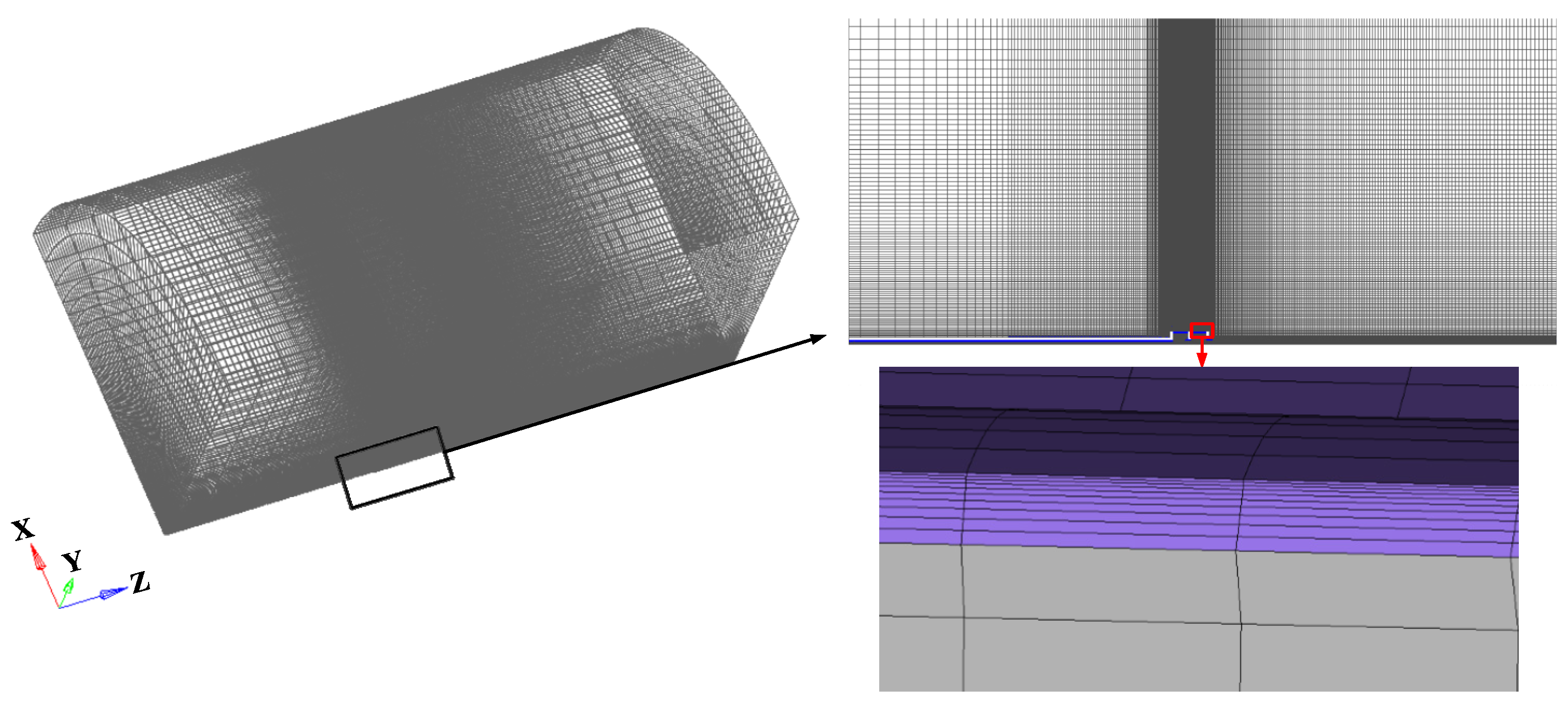
3.1. Numerical Setup

A large calibre machine gun with a typical muzzle brake, as shown in Figure 2, was taken as the research object. Based on the circumferential symmetry of its structure, the analysis is focus on the quarter of the object geometry, which leads to a minimal number of grids and improved computational efficiency. The computational domain is performed in Figure 3, where d is the muzzle diameter. The positive direction of Z axis represents the jet direction and the central point of bore bottom section is set as the coordinate origin.

The boundary conditions are displayed in Figure 3a. The separate boundaries of no-slip wall (in gray) and pressure-outlet (in pink) are set for the outer surfaces and muzzle flow field domain, respectively. In addition, the symmetry plane was set as the symmetry boundary condition (in yellow). The start time of calculation was set to the end of the interior ballistics, which represents the initial flow of propellant gas after the projectile leaves the muzzle. The initial distribution of pressure and velocity in the chamber, as shown in Figure 4, were calculated by the internal ballistics equations [22], and the temperature inside the bore was set as an average value of 2000 K. While the area outside the bore was the atmospheric condition of 300 K and 101,325 Pa.

3.2. Numerical Method

The calculation process involves two steps, as shown in Figure 5. Firstly, in the CFD part, the unsteady flow of turbulence is modelled by the LES method. After the quasi-stationary flow state is reached, the sound pressure at the receiving position is determined by the FW-H acoustic analogy equation based on the source data obtained from the LES results of acoustic integration surface. The location of the FW-H surfaces is shown in Figure 3b. Several sound receivers varying with radius and angles are demonstrated in Figure 6, where r = 2 m and θ varies every 10° following the counterclockwise direction of the downstream jet in the range of 0°~150°. ANSYS FLUENT 19.0 software is used for the numerical simulations. The flux calculation is carried out with a 3nd order MUSCL method and an AUSM flux scheme. The time integration is performed with an implicit 2nd order Runge-Kutta scheme. The parameters of unsteady flow field on the integral surface were collected every 5 time steps (Δ t = 2.50 × 10⁻⁶ s), which results in a total time of 0.025 s.

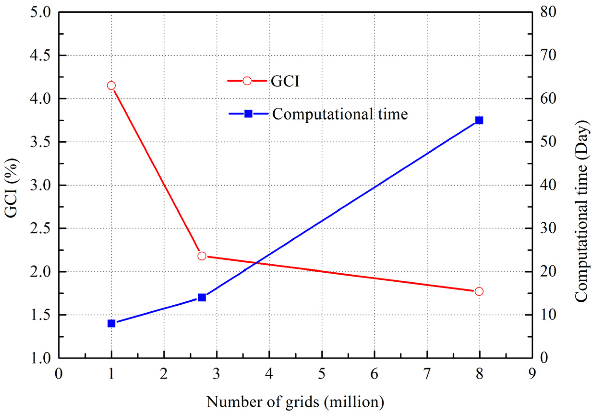
3.3. Grid Convergence Study

The resolution of muzzle flow and noise fields was improved using the structured mesh as grid topology. The first boundary layer was obtained by y⁺ = 1 and the other 9 layers were created with a growth rate of 1.2. Additionally, the grids away from the jet region are coarsened so that the acoustic waves cannot reach the external boundaries to avoid spurious reflexions. The grid convergence was further studied to determine the mesh size by evaluating the Grid Convergence Index [23,24]. Three sets of grids with different densities were generated as presented in

Table 1. Grid mesh parameters.

	Type	Number of Grid Cells	Average Skewness
1	Coarse	1,001,200	0.85
2	Medium	2,720,810	0.88
3	Fine	7,989,430	0.90

. Grid 2 and Grid 3 refined the mesh near the region of muzzle brake and jet flow on the basis of the same topology structure as Grid 1. The grid model of Grid 2 was displayed in Figure 7 as an example.

The grid convergence was verified by taking the pressure as the variable and the value of points at r = 0.2 m, θ = 30°, 60° and 90° on the XZ plane, which were set as P1, P2 and P3, respectively, were calculated. The results of GCI are shown in

Table 2. Calculated results of GCI.

Point	Grid	Pressure/Pa	GCI
P1	1	103,391.9	4.03%
	2	101,828.6	2.12%
	3	101,507.5	1.72%
P2	1	102,995.9	3.54%
	2	101,626.2	1.86%
	3	101,344.8	1.51%
P3	1	103,721.8	4.89%
	2	101,831.2	2.56%
	3	101,443.2	2.08%

. It can be seen that the GCI at all three points decreases with the increase of grid density. This observation is consistent with the situation that the denser the grid is, the closer the discretization result is to the exact solution and the smaller the discretization error is, indicating that the grid encryption is reasonable. According to the grid convergence index criterion [23,24], the grid can be considered to have reached convergence if the GCI of two continuous grids is less than 3%, therefore, the results of the second and third grids met the requirements of grid convergence, and that is, the results of numerical simulation are independent of the grid.

3.4. Computational Cost

The computing platform with 10 independent nodes connected by Infiniband was used in this study. Each node has two 6-core processors and 48 GB of local memory. Comparison between computational time and GCI of three sets is shown in Figure 8. The GCI of Grid 2 demonstrates a similar performance to that of a more refined Grid 3, but only one-fifth of the computation time is required. Thus, the mesh size of Grid 2 with 2.72 million three-dimensional grid cells was used in our study.

4. Model Validation

4.1. Numerical Results

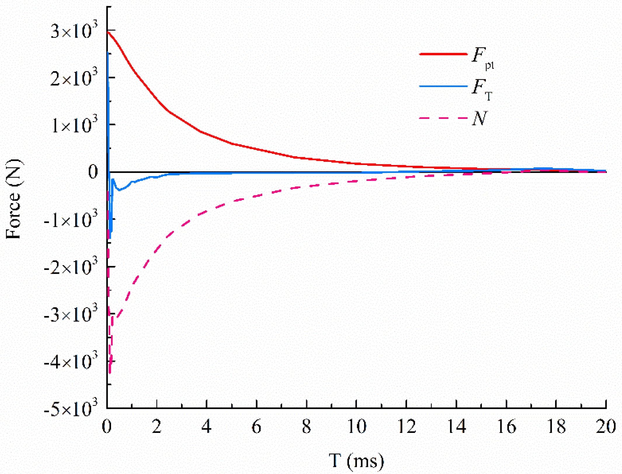
4.1.1. Muzzle Brake Efficiency

The stress analysis diagram of the recoil part is shown in Figure 9, where F_pt is the force at the bottom of the bore, and N is the reaction force caused by the muzzle brake. Without a muzzle brake, the barrel is only affected by F_pt and once a muzzle brake is installed, the reaction force N from muzzle brake should also be included, that is, the resultant force of free recoil part F_T = F_pt + N.

According to the definition of muzzle brake efficiency, it can be calculated by:

$${\eta }_T=1-\frac{M_0}{M_1}\frac{{\left(q{v}_0+{\beta }_T\omega v_0\right)}^2}{{\left(q{v}_0+\beta \omega v_0\right)}^2}$$

(6)

where M₀ and M₁ are the mass of free recoil part without and with a muzzle brake, respectively; q is the mass of projectile; v₀ is the initial velocity of projectile; ω is the charge of propellant; β and β_T are the function coefficient of propellant gas without and with a muzzle brake, respectively. The calculation equations are expressed as:

$$\beta =0.5+\frac{{\displaystyle {\int }_0^{\tau }{F}_{pt}dt}}{\omega v_0}$$

(7)

$${\beta }_T=0.5+\frac{{\displaystyle {\int }_0^{\tau }{F}_{T}dt}}{\omega v_0}$$

(8)

As the numerical simulation is unsteady and lasts for the whole after-effect period, the total impulse I₀ and I_n under the two conditions can be integrated through the force obtained during the simulation as:

$$I_0={\displaystyle {\int }_0^{\tau }{F}_{pt}dt}$$

(9)

$$I_n={\displaystyle {\int }_0^{\tau }{F}_{T}dt}$$

(10)

By sorting out Equation (6), the calculation formula of muzzle brake efficiency based on simulated results can be described as:

$${\eta }_T=1-\frac{M_0{\left[\left(q+0.5\omega \right)v_0+I_n\right]}^2}{M_1{\left[\left(q+0.5\omega \right)v_0+I_0\right]}^2}$$

(11)

The forces varying with time during the after-effect period is shown in Figure 10. According to the force curves, it can be seen that the initial value of F_pt was large and decreased with the continuous outflow of propellant gas, eventually reaching equilibrium close to the atmospheric pressure. The reaction force N had the opposite direction to F_pt and exceeded its value in a very short time. Therefore, the resultant force F_T exerted on the barrel compensated the recoil force and reduced the recoil speed, thus eliminating the recoil.

The total impulse I₀ and I_n were computed by the integration of F_T and F_pt with time, respectively, as shown in Figure 11. According to Figure 10, t = 18 ms, when the pressure in the barrel equals to atmospheric pressure, was considered as the moment at which the chamber empties gas at. Thus, the corresponding value of impulse was used to calculate the muzzle brake efficiency. Taking the mass of projectile q = 0.0482 kg, the charge amount ω = 0.017 kg, and assuming that the recoil mass with and without muzzle brake was approximately equal, the muzzle brake efficiency was calculated by Equation (11) to be 29.02%.

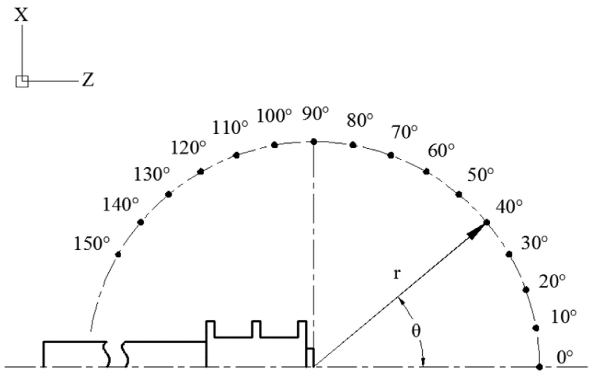
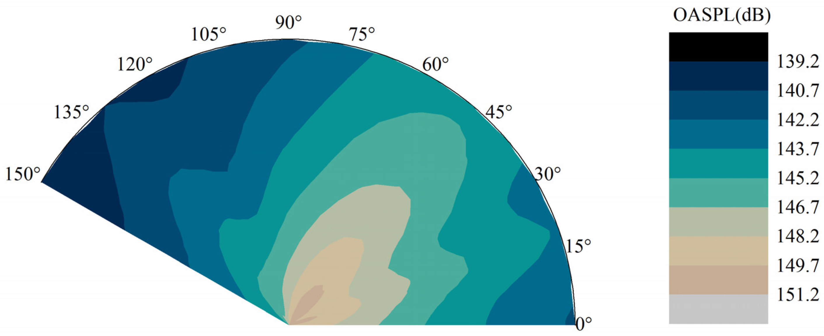
4.1.2. Muzzle Impulse Noise

The Sound Pressure Level (SPL) was determined by the following correlation:

$$SPL=20{\log }_{10}\frac{p^{\prime }}{p_{ref}}$$

(12)

$$OASPL=10{\log }_{10}\left({\displaystyle \sum _i{10}^{\frac{SP{L}_i}{10}}}\right)$$

(13)

where p′ is the sound pressure, p_ref is the reference sound pressure, taking p_ref = 2 × 10⁻⁵ Pa; SPL_i is the sound pressure level from the ith harmonic wave.

The calculated noise directivity map and OASPL distribution are shown in Figure 12. As can be seen from the figure, the muzzle impulse noise field demonstrated obvious directivity with the instalment of a muzzle brake. The sound energy was mostly concentrated in the azimuth range of θ = 40° to 70°, and reached the maximum value at the position of θ = 50°. Furthermore, it can be observed that the OASPL increased at θ = 135° due to the shunt effect of the side hole, making the influence area of the gas jet extend to the side and rear of the barrel.

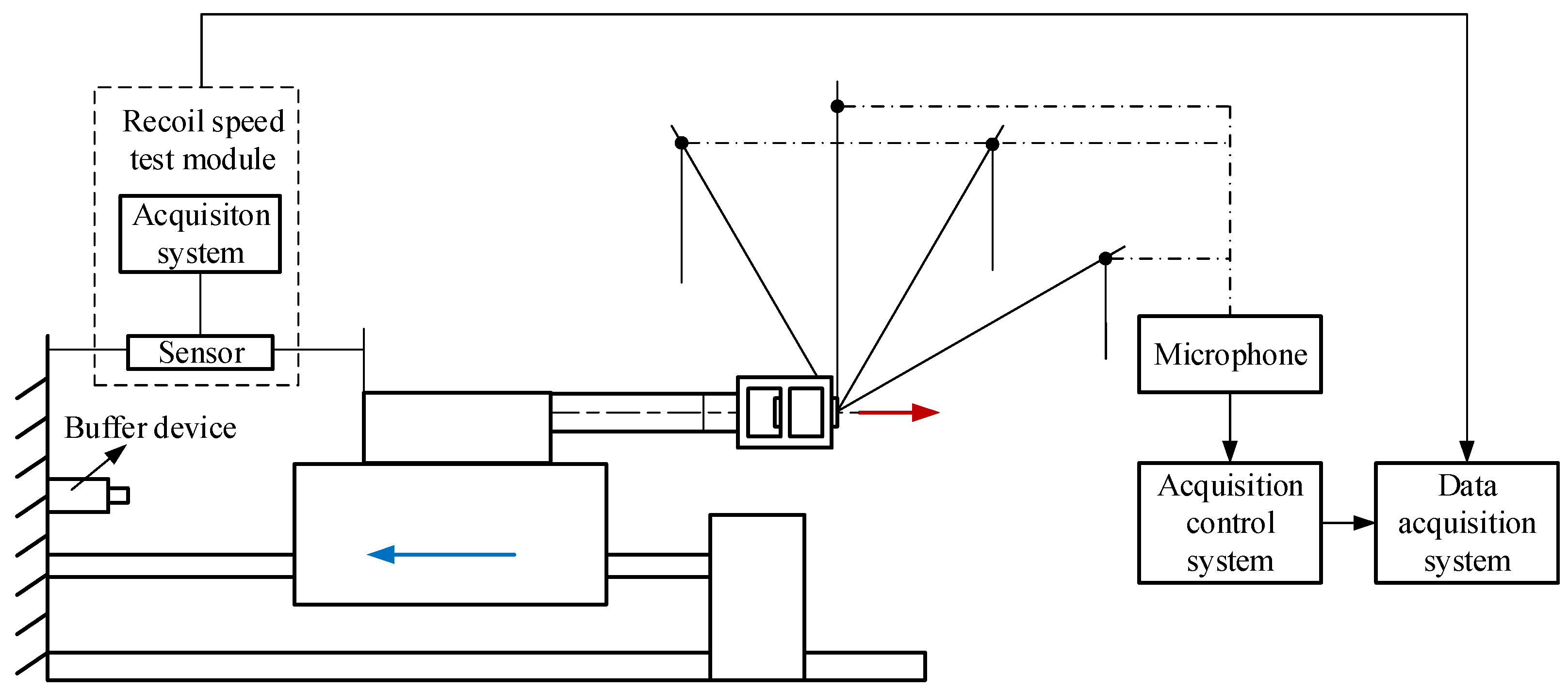
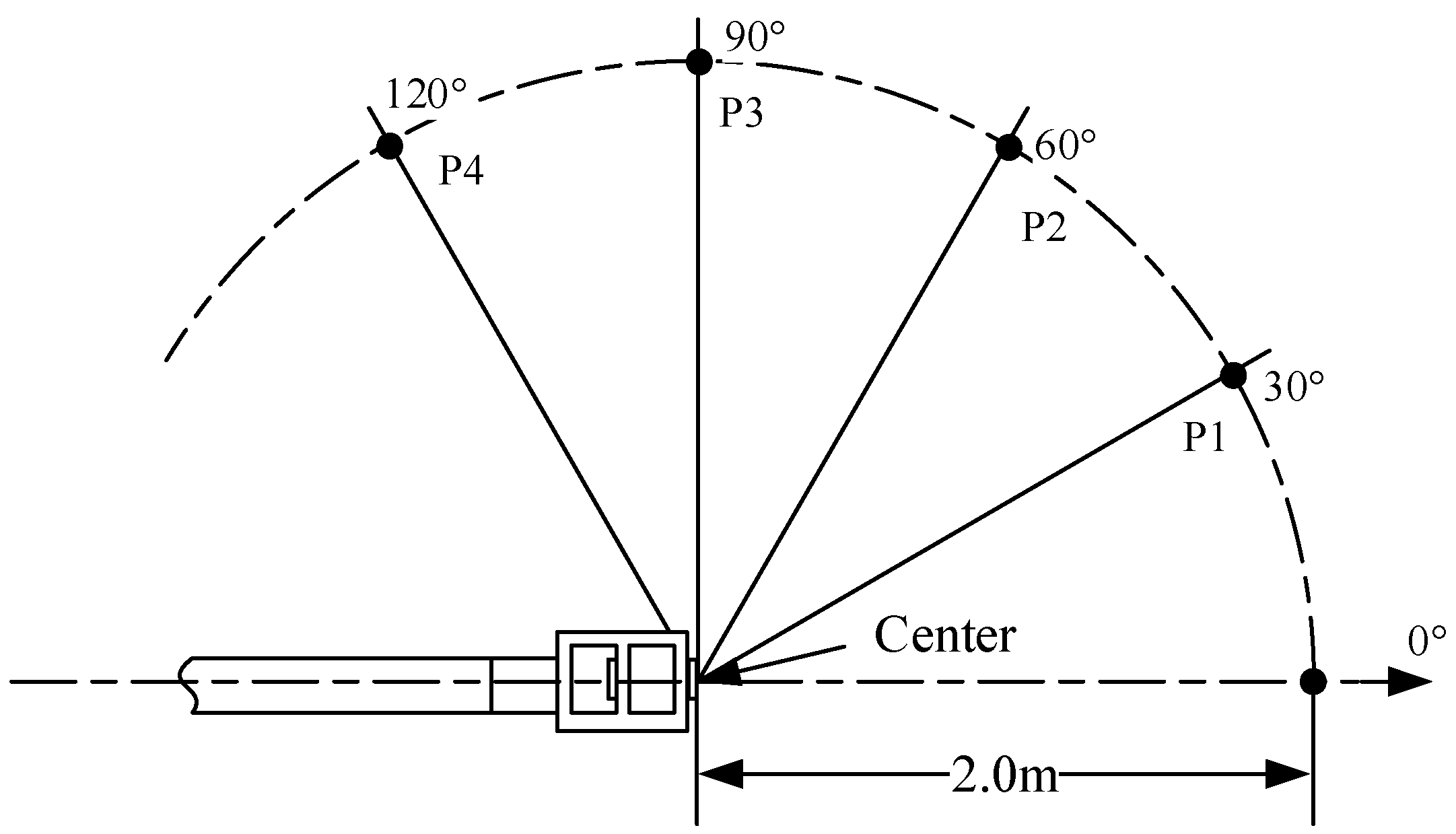
4.2. Experimental Setup

In order to verify the numerical method in current study, a corresponding experiment was conducted in a 150 m outdoor target. The experiment was divided into two parts; the muzzle brake efficiency and the impulse noise were tested, respectively. The schematic diagram of experimental scheme is shown in Figure 13. The test system mainly consisted of recoil speed test module, microphones, an acquisition control system with data preprocessing module and a data acquisition system with post-processing module.

The value of braking efficiency is obtained based on the method of measuring the maximum free recoil speed. During the test, the weapon was placed on the free recoil mount. While the weapon was fired and the projectile moved forward (as shown by the red arrow), the free recoil part moved backward (as shown by the blue arrow) due to the recoil force. The acquisition system connected with the sensors was used as a recoil speed test module to collect the free recoil speed, and the muzzle brake efficiency was further calculated based on the test data. Ten single shots were fired and recorded with and without a muzzle brake. The formula for calculating muzzle brake efficiency based on the experimental data is expressed as:

$${\eta }_T=1-\frac{M_1{V}_1{}^2}{M_0{V}_0{}^2}$$

(14)

where M₀ and M₁ are the mass of free recoil part without and with a muzzle brake, respectively; V₀ and V₁ are the average recoil velocity for ten rounds of free recoil part without and with a muzzle brake, respectively.

When the noise test was conducted, a tripod support was used to replace the free recoil mount and the sound pressure signals were, respectively, measured with radius of 2.0 m at 0°, 30°, 60°, 90° and 120° counterclockwise from the downstream direction of the jet, as shown in Figure 14. The BSWA MA421 quarter-inch free field high intensity microphones without the foam windscreen were selected, all of which were connected to the acquisition control system, SIRIUS-HS 8xCHG of DEWESoft Company. The microphones were mounted on a weighted tripod to make sure the axis vertical to the ground and the height horizontal to the gun barrel axis. The signal of individual shots was recorded by DEWESoftx2 software at a sampling frequency of 102,400 Hz.

4.3. Comparison of Simulated and Experimental Results

The comparison results of muzzle brake efficiency are shown in

Table 3. Comparison between the calculated and experimental results of muzzle brake efficiency.

	Measured	Calculated	Difference/%
muzzle brake efficiency/%	29.7	29.02	2.29

.

The experimental data collected by the microphones from various measurement points was processed by wavelet analysis method [17,25,26] and the average OASPL for 10 rounds at all the measurement points after processing is shown in

Table 4. Comparison between the calculated and experimental results of OASPL.

Point (r = 2.0 m)	θ/°	OASPL/dB		Difference/%
		Measured	Calculated
P1	30	149.75	142.95	−4.54
P2	60	150.63	144.05	−4.37
P3	90	148.87	141.78	−4.71
P4	120	147.20	140.56	−4.51

, together with the comparison with the calculated results.

The deviations between the calculated and measured data of the muzzle brake efficiency and OASPL are both within 5%, suggesting that the simulation method can be applied to practical scenarios.

5. Comprehensive Performance Evaluation of Muzzle Brakes with Various Structures

The verified method was further used to evaluate the comprehensive performance of three differently structured muzzle brakes, targeting muzzle brake efficiency and OASPL of muzzle impulse noise as the design indexes at the same time.

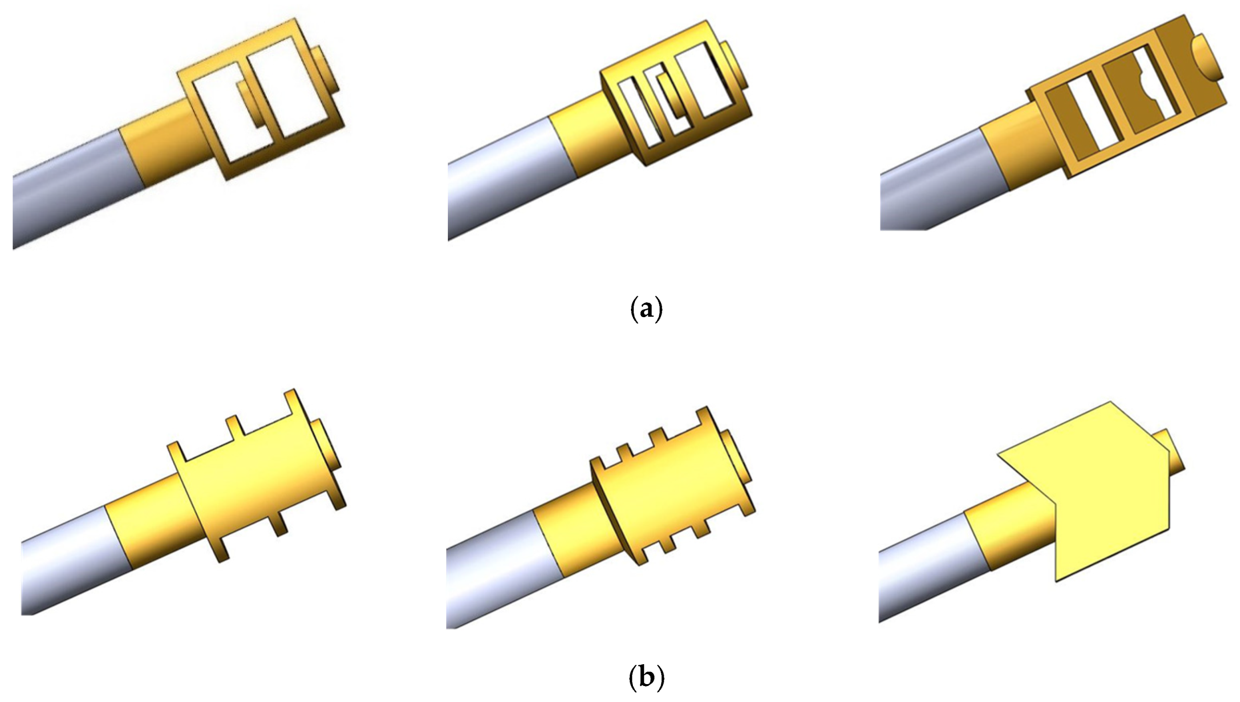
5.1. Design Details and Numerical Setup

Three muzzle brakes with various structures are visualized in Figure 15. The first one is the common cylindrical muzzle brake with two-cavities and double-rows. The second one increases the complexity as three-cavity multi-row cylindrical structure. The cavity half cone angle is reduced correspondingly from 90° to 73°. The last type instead of cylindrical design chooses inverted V-shaped with two chambers, double rows, and the cavity half cone angle of 115°.

The validated model is used for simulation. The numerical setup such as the initial and boundary conditions are the same as that in Section 3.1. The sound receiving points located at 0.5 m, 1.0 m and 2.0 m to the left of the shooter’s head to assess the negative impact of noise, as shown in Figure 16.

5.2. Results and Discussion

The Mach number contour distribution over time inside the muzzle brake for different structures are visualized in Figure 17, Figure 18 and Figure 19. As the simplest structure, the first muzzle brake clearly demonstrates the recoil compensation processes, as shown in Figure 17. The propellant gas impacts the reflection baffle when expanding through the two cavities, which results in the concentration of the pressure in the front wall of the muzzle brake and generation of the force opposite to the recoil force. The second muzzle brake is relatively more complex, as shown in Figure 18. Most of the high pressure is concentrated on the front wall of the second cavity with more severe fluctuations. As for inverted V-shaped muzzle brake in Figure 19, it has the highest efficiency because of the maximum contact area between the muzzle brake and the propellant gas. It can be observed that with the rapid expansion, the propellant gas hits the reflection baffle with faster speed reduction and greater reaction force.

Pressure and velocity contours of the flow field for three muzzle brakes are distributed in Figure 20 and Figure 21, respectively. The value evolutes over time and they differ based on different structures of muzzle brakes. It can be noticed that at t = 0.25 ms, individual shock waves are formed for each side hole jet with corresponding exit parameter and angle. Due to the relatively small distance between side holes, jet boundaries cross to each other and the bottle-shaped shock waves in the side holes interact to form a larger shock bottle after 0.25 ms. The shock waves are continuing developing which can be observed at bullet hole and side hole positions when time passes 0.75 ms. Afterwards, the decay period starts as can be seen at time equals to 2.5 ms. It can be concluded that the muzzle brake structure has large influence on pressure and velocity. The inverted V-shaped structure has the most obvious recoil effect as the angle between the direction of airflow in the side hole and the jet axis is greater than 90°. Thus, the propellant gas is directed to the rear of the muzzle brake to produce a larger reaction force. As for the cylindrical muzzle brakes, the second type is preferable with stronger bullet hole jet and more uniform bottle-shaped shock waves, which leads to a greater recoil compensation.

The resultant force F_T on the barrel is plotted in Figure 22. The largest reversing force is created by installing V-shaped muzzle brake. Therefore, such type of muzzle brake can effectively reduce the weapon’s free recoil speed and has a higher efficiency. Despite of small discrepancies, the similar trend of forces can be observed for the two cylindrical muzzle brakes. The main difference is at the beginning of after-effect period and type 2 creates a larger force. The efficiency and OASPL at the designated sound receiving point of the three muzzle brakes are shown in

Table 5. Comparison of muzzle brake efficiency and comprehensive noise performance.

	Muzzle Brake Efficiency/%	Point A (r = 0.5 m)		Point B (r = 1.0 m)		Point C (r = 2.0 m)
		OASPL/dB	Difference	OASPL/dB	Difference	OASPL/dB	Difference
Without	-	141.31	-	141.56	-	137.46	-
Type1	29%	143.54	2.23	143.24	1.68	142.24	4.78
Type2	31%	140.90	−0.41	143.49	1.93	146.07	8.61
Type3	37%	142.64	1.33	145.53	3.97	144.75	7.29

.

Based on the analysis above, it can be observed that the structure parameters, such as the side hole shape and opening angle, have direct influence on the propellant gas distribution in the internal area and structure of the muzzle flow field, thereby affecting the brake efficiency and directivity of noise. Only from the perspective of braking efficiency, the third muzzle brake is the best; from the influence of impulse noise, almost all of the points have increased OASPL after the instalment of a muzzle brake, but the third type has the greatest impact on the noise in the left side of the shooter compared with the case without a muzzle brake. To further evaluate the comprehensive performance, an evaluation index Z_T is defined as:

$$Z_T\left(n\right)={\omega }_1{f}_1\left(n\right)+{\displaystyle \sum }_{i=2}^k{\omega }_i{f}_i\left(0\right)/f_i\left(n\right)$$

(15)

where n is the type number; f_i (n) is the evaluation index of each sub target; f₁ is the braking efficiency and f₂~f_k are the sound pressure level at different points, which are normalized according to the case without a muzzle brake, defined as n = 0 to be the standardized reference. ω_i is the weight coefficient and ${\displaystyle \sum _{i=1}^k{\omega }_i=1}$. According to the previous research experience, the muzzle brake efficiency is the main performance index, so it is taken here ω₁ = 0.7, ω₂ = 0.15, ω₃ = 0.1, and ω₄ = 0.05. The calculated Z_T of three muzzle brakes is 0.50, 0.51 and 0.55, respectively. According to the definition of Z_T, the higher value, the better comprehensive performance. Therefore, it can be concluded that among the three types, the V-shaped muzzle brake of type 3 is preferable.

6. Conclusions

In this paper, a comprehensive performance evaluation method targeting muzzle brake efficiency and impulse noise based on the LES/FW-H numerical method was proposed. As a result of this study, the concluding remarks are made as:

(1) There is a good agreement between the numerical results and the experimental data and it is obvious that the method proposed in this paper is feasible;

(2) For the evaluated three types, the installation of muzzle brakes will inevitably cause the change of the noise value at the same measuring point, but the relationship between the changes of brake efficiency and OASPL is not a simple linear function.

The comprehensive performance evaluation method based on the numerical simulation is highly recommended for preliminary design and optimization of muzzle brakes. Further analysis can be carried out according to the changes influenced by a single structural parameter of muzzle brakes, which can provide a reference for its structural optimization.

References

1. Ramezanizadeh, M.; Puia, A.; Ahmadi, M.; Chau, K.-w. Experimental and numerical analysis of a nanofluidic thermosyphon heat exchanger. Eng. Appl. Comput. Fluid Mech. 2019, 13, 40–47. [Google Scholar] [CrossRef]
2. Abadi, A.M.; Sadi, M.; Farzaneh-Gord, M.; Ahmadi, M.H.; Chau, K.-w. A numerical and experimental study on the energy efficiency of a regenerative Heat and Mass Exchanger utilizing the counter-flow Maisotsenko cycle. Eng. Appl. Comput. Fluid Mech. 2020, 14, 1–12. [Google Scholar] [CrossRef] [Green Version]
3. Kim, Y.H.; Lee, M.; Hwang, I.J.; Kim, Y.J. Noise Reduction of an Extinguishing Nozzle Using the Response Surface Method. Energies 2019, 12, 4346. [Google Scholar] [CrossRef] [Green Version]
4. Nishad, K.; Ries, F.; Li, Y.; Sadiki, A. Numerical Investigation of Flow through a Valve during Charge Intake in a DISI—Engine Using Large Eddy Simulation. Energies 2019, 12, 2620. [Google Scholar] [CrossRef] [Green Version]
5. Sakamoto, K.; Matsunaga, K.; Fukushima, J.; Tanaka, A. Numerical analysis of the propagating blast wave in a firing range. In Proceedings of the 19th International Symposium in Ballistic, Interlaken, Switzerland, 7–11 May 2001; pp. 289–296. [Google Scholar]
6. Cler, D.L.; Chevaugeon, N.; Shephard, M.S.; Flaherty, J.E.; Remacle, J. Computational fluid dynamics application to gun muzzle blast—A validation case study. In Proceedings of the 41st Aerospace Sciences Meeting and Exhibit, Reno, Nevada, 6–9 January 2003. [Google Scholar] [CrossRef]
7. Cayzac, R.; Carette, E.; Patry, J.N. Computational Fluid Dynamics and Experimental Validations of the Direct Coupling Between Interior, Intermediate and Exterior Ballistics Using the Euler Equations. J. Appl. Mech. 2011, 78, 1774–1800. [Google Scholar] [CrossRef]
8. Chen, M.; Li, Z.; Mi, B. A Study of Muzzle Brake Structure Characteristics Based on CFD. Ordnance Ind. Autom. 2013, 32, 4–7. [Google Scholar] [CrossRef]
9. Zhang, H.; Chen, Z.; Jiang, X.; Li, H. Investigations on the exterior flow field and the efficiency of the muzzle brake. J. Mech. Sci. Technol. 2013, 27, 95–101. [Google Scholar] [CrossRef]
10. Gao, J.; Liu, S.H. Computation Methods of Muzzle Brake Efficiency. Mech. Eng. Autom. 2013, 2013, 176–177. [Google Scholar] [CrossRef]
11. Lee, I.C.; Lee, D.J.; Ko, S.H.; Dong, S.L.; Kang, G.J. Numerical analysis of a blast wave using CFD-CAA hybrid method. In Proceedings of the 12th Aiaa/Ceas Aeroacoustics Conference, Cambridge, MA, USA, 8–10 May 2006. [Google Scholar] [CrossRef] [Green Version]
12. Wang, Y.; Jiang, X.H.; Yang, X.P.; Guo, Z.Q.J.E.; Waves, S. Numerical simulation on jet noise induced by complex flows discharging from small caliber muzzle. Explos. Shock Waves 2014, 34, 508–512. [Google Scholar] [CrossRef]
13. Bogey, C.; Marsden, O.; Bailly, C. Effects of moderate Reynolds numbers on subsonic round jets with highly disturbed nozzle-exit boundary layers. Phys. Fluids 2012, 24, 53. [Google Scholar] [CrossRef] [Green Version]
14. Wan, Z.H.; Zhou, L.; Yang, H.H.; Sun, D.J. Large eddy simulation of flow development and noise generation of free and swirling jets. Phys. Fluids 2013, 25, 564–587. [Google Scholar] [CrossRef]
15. Bogey, C.; Marsden, O.; Bailly, C. Influence of initial turbulence level on the flow and sound fields of a subsonic jet at a diameter-based Reynolds number of 105. J. Fluid Mech. 2012, 701, 352–385. [Google Scholar] [CrossRef] [Green Version]
16. Brès, G.A.; Jaunet, V.; Rallic, M.L.; Jordan, P.; Colonius, T.; Lele, S.K. Large eddy simulation for jet noise: The importance of getting the boundary layer right. In Proceedings of the Aiaa/Ceas Aeroacoustics Conference, Dallas, TX, USA, 22–26 June 2015. [Google Scholar] [CrossRef] [Green Version]
17. Zhao, X.Y.; Zhou, K.D.; HE, L.; LU, Y.; Li, J.S. Wavelet Analysis and Numerical Simulation of Jet Noise induced by a Large Caliber Small Arms. Acta Armamentarii 2019, 40, 2195–2203. [Google Scholar] [CrossRef]
18. Zhao, X.Y.; Zhou, K.D.; He, L.; Lu, Y.; Zheng, Q. Numerical Simulation and Experiment on Impulse Noise in a Small Caliber Rifle with Muzzle Brake. Shock Vib. 2019, 2019, 1–12. [Google Scholar] [CrossRef]
19. Rodi, W. Turbulence Modeling and Simulation in Hydraulics: A Historical Review. J. Hydraul. Eng. 2017, 143, 03117001. [Google Scholar] [CrossRef]
20. Lilly, D.K. A proposed modification of the Germano subgrid-scale closure method. Phys. Fluids A Fluid Dyn. 1998, 4, 633–635. [Google Scholar] [CrossRef]
21. Ffowcs Williams, J.E.; Hawkings, D.L. Sound Generation by Turbulence and Surfaces in Arbitrary Motion. Philos. Trans. R. Soc. Lond. Ser. A Math. Phys. Sci. 1969, 264, 321–342. [Google Scholar] [CrossRef]
22. Carlucci, D.E.; Jacobson, S.S. Interior Ballistics; Taylor and Francis: Oxford, UK, 2014; p. 2014. [Google Scholar]
23. Roache, P. Error bars for CFD. In Proceedings of the 41st Aerospace Sciences Meeting and Exhibit, Reno, Nevada, 6–9 January 2003. [Google Scholar] [CrossRef]
24. Manna, P.; Dharavath, M.; Sinha, P.K.; Chakraborty, D. Optimization of a flight-worthy scramjet combustor through CFD. Aerosp. Sci. Technol. 2013, 27, 138–146. [Google Scholar] [CrossRef]
25. Carter, P.H. Unknown transient detection using wavelets. Wavelet Appl. 1994, 2242, 137–149. [Google Scholar] [CrossRef]
26. Zhou, F.; Jiang, Y.; Zhang, X.; Hao, J. Time-frequency Analysis of Test Data from Complex Noise of Rocket Engine Jet. J. Proj. Rocket. Missiles Guid. 2012, 32, 145–147. [Google Scholar] [CrossRef]
Figure 1. Steps of traditional design methods.
Energies 15 03576 g001
Figure 2. Schematic diagram of muzzle brake. (a) 3D view. (b) Top view (section).
Energies 15 03576 g002
Figure 3. Computational domain and boundary conditions. (a) 3D view. (b) Section view.
Energies 15 03576 g003
Figure 4. Initial conditions.
Energies 15 03576 g004
Figure 5. Flow chart of the CFD-CAA hybrid method.
Energies 15 03576 g005
Figure 6. Receiver locations in the far fields.
Energies 15 03576 g006
Figure 7. Computational grid model.
Energies 15 03576 g007
Figure 8. Comparison between computational time and GCI.
Energies 15 03576 g008
Figure 9. Force analysis of recoil part.
Energies 15 03576 g009
Figure 10. Force varying with time.
Energies 15 03576 g010
Figure 11. Impulse varying with time.
Energies 15 03576 g011
Figure 12. Direction diagram of OASPL on Plane XZ.
Energies 15 03576 g012
Figure 13. Schematic diagram of experimental scheme.
Energies 15 03576 g013
Figure 14. Measurement point locations in the far field.
Energies 15 03576 g014
Figure 15. Schematic diagram of muzzle brakes with three different structures. (a) Side view. (b) Top view.
Energies 15 03576 g015
Figure 16. Diagram of receiver locations.
Energies 15 03576 g016
Figure 17. Distribution of Mach number in muzzle brake of type 1. (a) t = 0.05 ms. (b) t = 0.10 ms. (c) t = 0.20 ms.
Energies 15 03576 g017
Figure 18. Distribution of Mach number in muzzle brake of type 2. (a) t = 0.05 ms. (b) t = 0.10 ms. (c) t = 0.20 ms.
Energies 15 03576 g018
Figure 19. Distribution of Mach number in muzzle brake of type 3. (a) t = 0.05 ms. (b) t = 0.10 ms. (c) t = 0.20 ms.
Energies 15 03576 g019
Figure 20. Pressure contour distribution of three different muzzle brake. (a) t = 0.25 ms. (b) t = 0.50 ms. (c) t = 0.75 ms. (d) t = 2.50 ms. (from left to right the muzzle brakes were defined previously as one to three types).
Energies 15 03576 g020
Figure 21. Velocity contour distribution of three different muzzle brake. (a) t = 0.25 ms. (b) t = 0.50 ms. (c) t = 0.75 ms. (d) t = 2.50 ms. (from left to right the muzzle brakes were defined previously as one to three types).
Energies 15 03576 g021
Figure 22. Force varying with time of three different muzzle brakes.
Energies 15 03576 g022