
Projecting and Forecasting the Latent Volatility for the Nasdaq OMX Nordic/Baltic Financial Electricity Market Applying Stochastic Volatility Market Characteristics


Abstract
:1. Introduction
2. Literature and Methodologies
3. Nordic/Baltic Electricity Market’s Front Year and Front Quarter Contracts
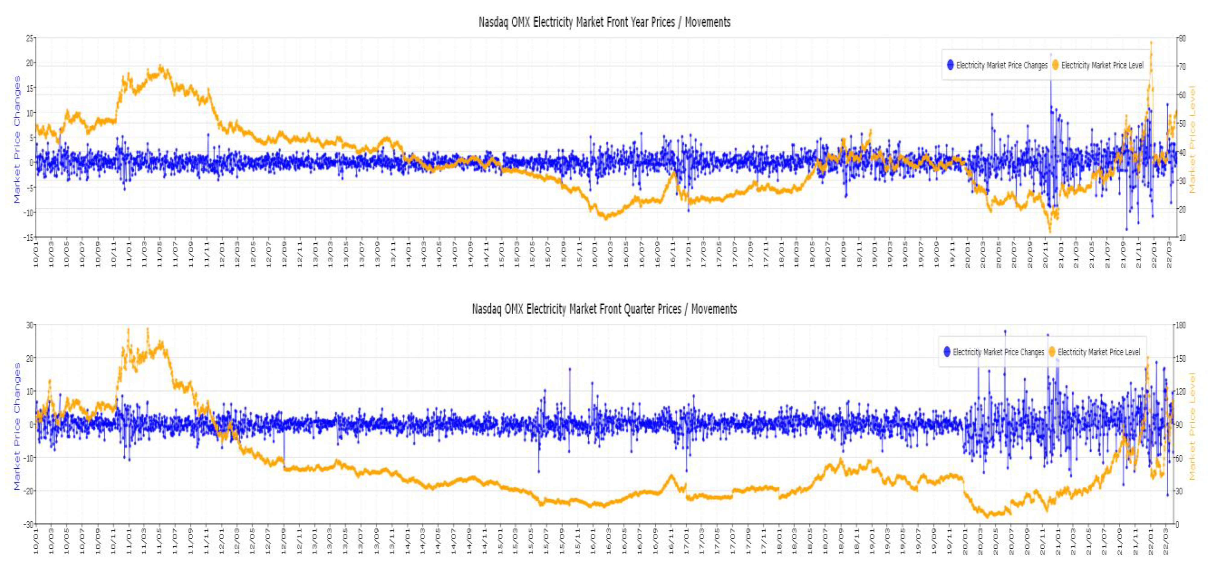
3.1. The Nasdaq OMX Front Year and Front Quarter Contracts
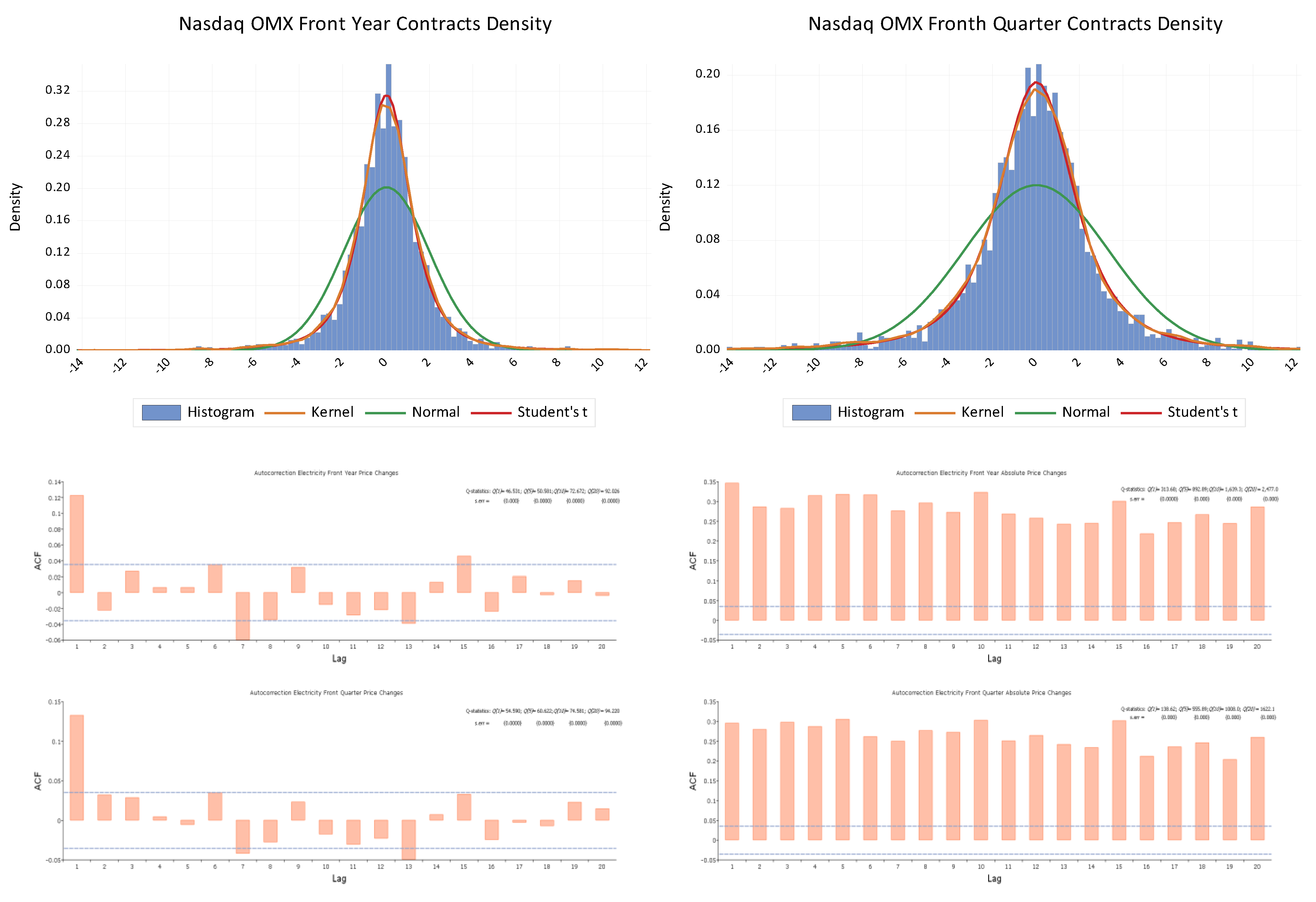
3.2. Empirical Results
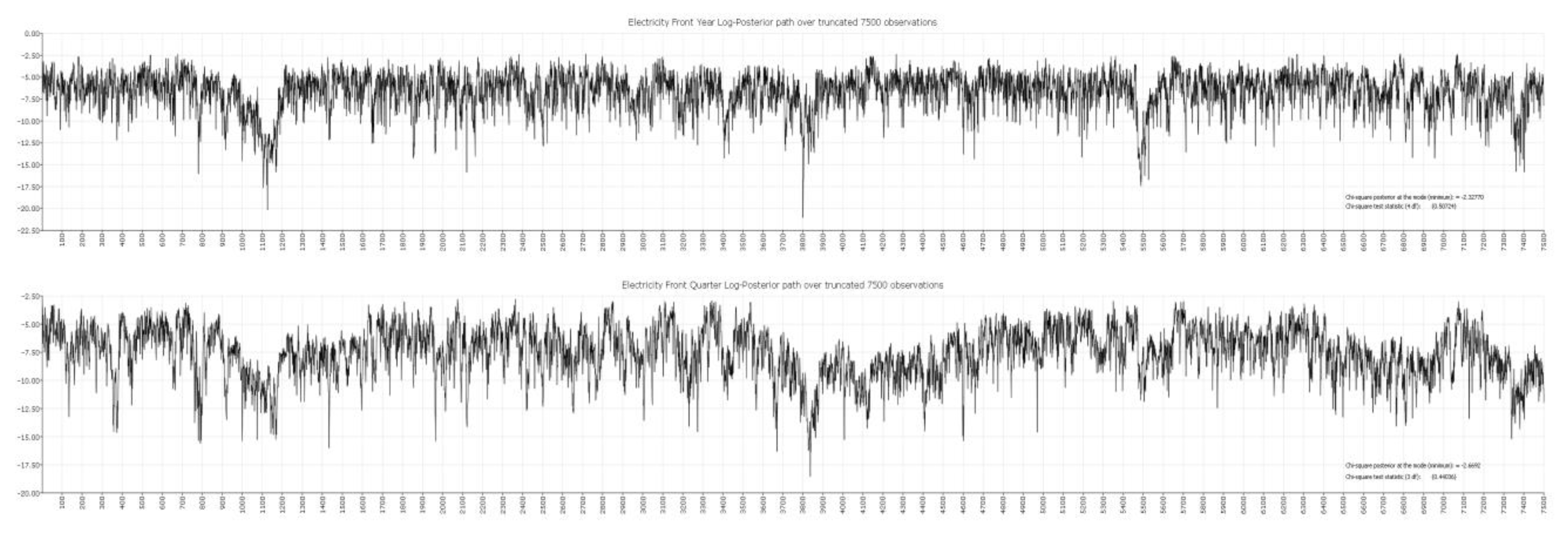
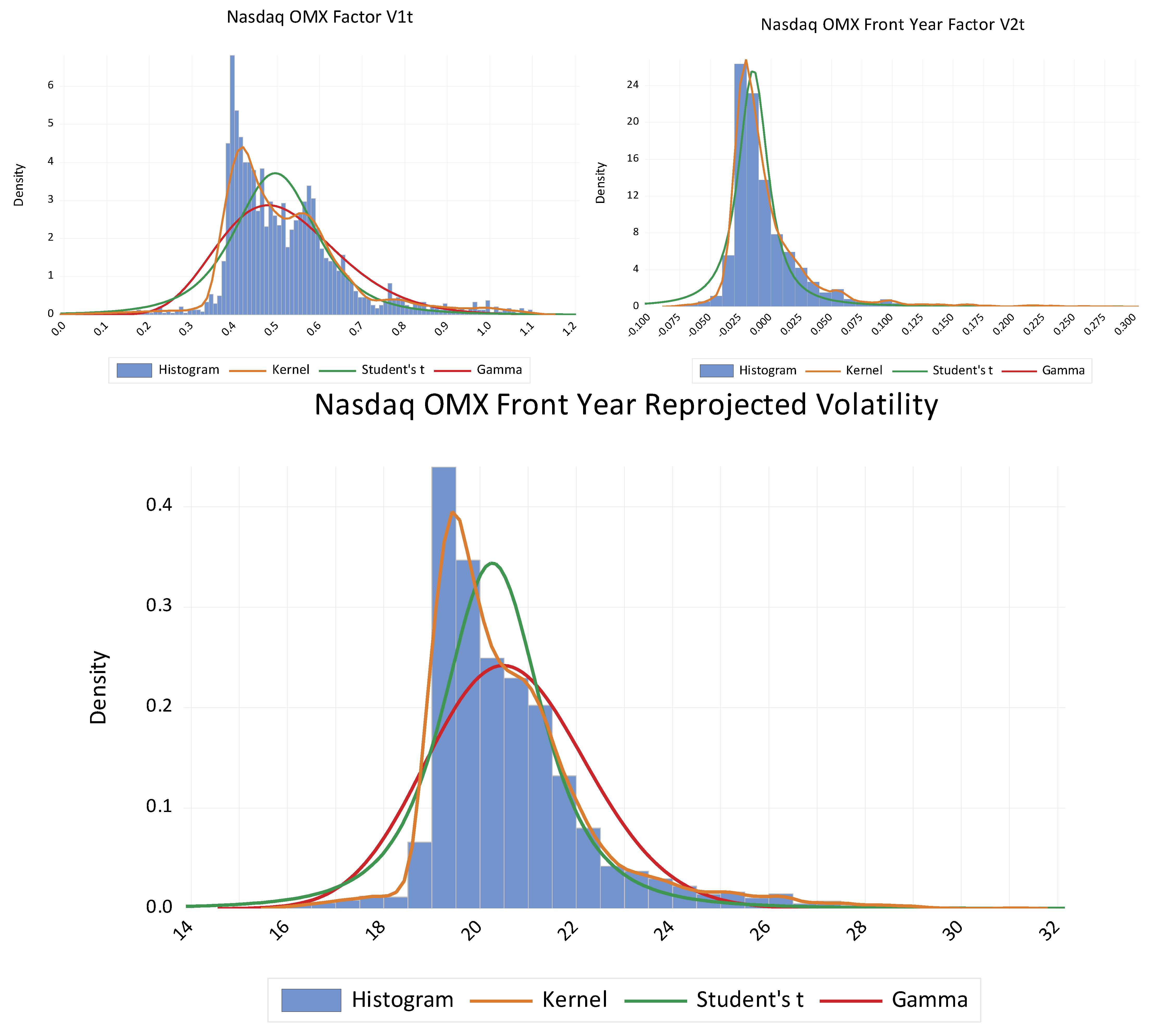
3.3. Nasdaq OMX Front Year and Front Quarter Stochastic Volatility
3.4. Forecasting Nasdaq OMX Front Year and Front Quarter Volatility
4. Discussion
4.1. Stochastic Volatility Characteristics
4.2. Stochastic Volatility Forecasts
5. Conclusions
Supplementary Materials
Funding
Conflicts of Interest
References
- Lo, A.W.; MacKinlay, C. Stock Market Prices Do Not Follow Random Walks: Evidence from a Simple Specification Test. Rev. Financ. Stud. 1988, 1, 41–66. [Google Scholar] [CrossRef]
- Taylor, S.J. Financial returns modelled by the product of two stochastic processes–a study of daily sugarprices 1961-79. In Time series Analysis: Theory and Practice 1; Andersen, O.D., Ed.; Elsevier Science Ltd.: Amsterdam, The Netherlands, 1982; pp. 203–226. [Google Scholar]
- Clark, P.K. A subordinated stochastic process model with fixed variance for speculative prices. Econometrica 1973, 412, 15–156. [Google Scholar]
- Hull, J.; White, A. The pricing of options on assets with stochastic volatilities. J. Financ. 1987, 42, 281–300. [Google Scholar] [CrossRef]
- Hansen, L.P. Large Sample Properties of Generalized Method of Moments Estimators. Econometrics 1982, 50, 1029–1054. [Google Scholar] [CrossRef]
- Gallant, A.R.; McCulloch, R.E. GSM: A Program for Determining General Scientific Models; Duke University: Durham, NC, USA, 2020; Available online: https://www.aronaldg.org/webfiles/arg/gsm (accessed on 1 April 2022).
- Gallant, A.R.; Tauchen, G. Reprojecting Partially Observed Systems with Application to Interest Rate Diffusions. J. Am. Stat. Assoc. 1998, 93, 10–24. [Google Scholar] [CrossRef]
- Gallant, A.R.; Tauchen, G. New Directions in Time Series Analysis, Part II. In A Nonparametric Approach to Nonlinear Time Series Analysis: Estimation and Simulation; Brillinger, D., Caines, P., Geweke, J., Parzan, E., Rosenblatt, M., Taqqu, M.S., Eds.; Springer: New York, NY, USA, 1992; pp. 71–92. [Google Scholar]
- Chernozhukov, V.; Hong, H. An MCMC Approach to Classical Estimation. J. Econom. 2003, 115, 293–346. [Google Scholar] [CrossRef] [Green Version]
- Andersen, T.G.; Benzoni, L.; Lund, J. Towards an empirical foundation for continuous-time models. J. Financ. 2002, 57, 1239–1284. [Google Scholar] [CrossRef] [Green Version]
- Andersen, T.G.; Bollerslev, T.; Diebold, F.X.; Labys, P. Modelling and Forecasting realized volatility. Econometrica 2003, 71, 579–625. [Google Scholar] [CrossRef] [Green Version]
- Chernov, M.; Gallant, A.R.; Ghysel, E.; Tauchen, G. Alternative models for stock price dynamics. J. Econom. 2003, 56, 225–257. [Google Scholar] [CrossRef] [Green Version]
- Solibakke, P.B. Stochastic Volatility Models Predictive Relevance for Equity Markets. In Theory and Applications of Time Series Analysis: Selected Contributions from ITISE 2019, 1st ed.; Valenzuela, O., Rojas, F., Herrera, L.J., Pomares, H., Rojas, I., Eds.; Springer International Publishing: Cham, Switzerland, 2020; p. 1. [Google Scholar]
- Solibakke, P.B. Scientific stochastic volatility models for the European carbon markets: Forecasting and extracting conditional moments. Int. J. Bus. 2014, 19, 63–98. [Google Scholar]
- Shephard, N.; Andersen, T.G. Stochastic Volatility: Origins and Overview. In Handbook of Financial Time Series; Mikosch, T., Kreiß, J.P., Davis, R., Andersen, T., Eds.; Springer: Berlin/Heidelberg, Germany, 2009. [Google Scholar] [CrossRef]
- Rosenberg, B. The Behavior of Random Variables with Nonstationary Variance and the Distribution of Security Prices. Research Program in Finance. University of California: Berkeley, UK, Unpublished paper. 1972. [Google Scholar]
- Tauchen, G.; Pitts, M. The price variability volume relationship on speculative markets. Econometrica 1983, 51, 485–505. [Google Scholar] [CrossRef] [Green Version]
- Gallant, A.R.; Hsieh, D.A.; Tauchen, G. Estimation of stochastic volatility models with diagnostics. J. Econom. 1997, 81, 159–192. [Google Scholar] [CrossRef] [Green Version]
- Andersen, T.G. Stochastic autoregressive volatility: A framework for volatility modelling. Math. Financ. 1994, 4, 75–102. [Google Scholar]
- Durham, G. Likelihood-based specification analysis of continuous-time models of the short-term interest rate. J. Financ. Econ. 2003, 70, 463–487. [Google Scholar] [CrossRef] [Green Version]
- Gallant, A.R.; Tauchen, G. Simulated Score Methods and Indirect Inference for Continuous Time Models. In Handbook of Financial Econometrics; Aït-Sahalia, Y., Hansen, L.P., Eds.; Springer: North Holland, The Netherlands, 2010; Chapter 8; pp. 199–240. [Google Scholar]
- Hamilton, J.D. Time Series Analysis; Princeton University Press: Princeton, NJ, USA, 1994. [Google Scholar]
- Csörgö, S.; Faraway, J. The Exact and Asymptotic Distributions of Cramer-von Mises Statistics. J. R. Stat. Soc. Sre. B 1996, 58, 221–234. [Google Scholar] [CrossRef]
- Kwiatowski, D.; Phillips, P.C.B.; Schmid, P.; Shin, T. Testing the null hypothesis of stationary against the alternative of a unit root: How sure are we that economic series have a unit root. J. Econom. 1992, 54, 159–178. [Google Scholar] [CrossRef]
- Dickey, D.A.; Fuller, W.A. Distribution of the estimators for autoregressive time series with a unit root. J. Am. Stat. Soc. 1979, 74, 427–431. [Google Scholar]
- Ramsey, J.B. Tests for Specification Errors in Classical Linear Least Squares Regression Analysis. J. R. Stat. Soc. Ser. B 1969, 31, 350–371. [Google Scholar] [CrossRef]
- Brock, W.A.; Dechert, W.D.; Scheinkman, J.A.; LeBaron, B. A test for independence based on the correlationdimension. Econom. Rev. 1996, 15, 197–235. [Google Scholar] [CrossRef]
- Andrews, D.W.K. Tests for Parameter Instability and Structural Change with Unknown Change Point. Econometrica 1993, 61, 821–856. [Google Scholar] [CrossRef] [Green Version]
- Bai, J.; Perron, P. Estimating and Testing Linear Models with Multiple Structural Changes. Econometrica 1998, 66, 47–78. [Google Scholar] [CrossRef]
- Gallant, A.R.; Tauchen, G. EMM: A Program for Efficient Methods of Moments Estimation; Duke University: Durham, NC, USA, 2020; Available online: https://www.aronaldg.org/webfiles/emm (accessed on 1 April 2022).
- Schwarz, G. Estimating the Dimension of a Model. Ann. Stat. 1978, 6, 461–464. [Google Scholar] [CrossRef]
- Ljung, G.M.; Box, G.E.P. On a Measure of Lack of Fit in Time Series Models. Biometrika 1978, 65, 297–303. [Google Scholar] [CrossRef]
- Godfrey, L.G. Misspecification Tests in Econometrics; Cambridge University Press: Cambridge, UK, 1988. [Google Scholar]
- Alexander, C.; Korovilas, D.; Kapraun, J. Diversification with volatility products. J. Int. Financ. Money 2016, 65, 213–235. [Google Scholar] [CrossRef]
- Doran, J.S. Volatility as an asset class: Holding VIX in a portfolio. J. Futures Mark. 2020, 40, 841–859. [Google Scholar] [CrossRef]
- Bašta, M.; Molnár, P. Long-term dynamics of the VIX index and its tradable counterpart VXX. J. Futures Mark. 2019, 39, 322–341. [Google Scholar] [CrossRef]
- Bordonado, C.; Molnar, P.; Samdal, S.R. VIX Exchange Traded Products: Price Discovery, Hedging and Trading Strategy. J. Futures Mark. 2017, 37, 164–183. [Google Scholar] [CrossRef]
- Gnedenko, D.V. Sur la Distribution limité du terme d’une série aléatoire. Ann. Math. 1943, 44, 423–453. [Google Scholar] [CrossRef]
- Heston, S.L. A closed-form solution for options with stochastic volatility with applications to bond and currency options. Rev. Financ. Stud. 1993, 6, 327343. [Google Scholar] [CrossRef] [Green Version]


| Panel A | Nasdaq OMX Front Year Return Series | ||||||||
| Mean (all)/ | Median | Max./ | Moment | Quantile | Quantile | Cramer | Serial dependence | VaR | |
| M (-drop) | Std.dev. | Min. | Kurt/Skew | Kurt/Skew | Normal | von-Mises | Q(12) | Q2(12) | (1; 2.5%) |
| 0.03775 | 0.00000 | 21.5520 | 9.9166 | 0.28524 | 9.1610 | 1333.80 | 34.736 | 566.72 | −6.394% |
| 0.03716 | 2.10427 | −13.4348 | 0.35853 | 0.04656 | {0.0102} | {0.0000} | {0.0010} | {0.0000} | −4.452% |
| BDS-Z-statistic (e = 1) | Phillips & | Augment | ARCH | RESET | CVaR | ||||
| m = 2 | m = 3 | m = 4 | m = 5 | m = 6 | Perron | DF-test | (12) | (6;12) | (1; 2.5%) |
| 10.7530 | 12.7224 | 15.3246 | 18.0319 | 0.11584 | −44.57339 | −44.6405 | 252.848 | 4.189406 | −8.389% |
| {0.0000} | {0.0000} | {0.0000} | {0.0000} | {0.1246} | {0.0000} | {0.0000} | {0.0000} | {0.0000} | −6.517% |
| Panel B | Nasdaq OMX Front Quarter Return Series | ||||||||
| Mean (all)/ | Median | Max./ | Moment | Quantile | Quantile | Cramer- | Serial dependence | VaR | |
| M (-drop) | Std.dev. | Min. | Kurt/Skew | Kurt/Skew | Normal | von-Mises | Q(12) | Q2(12) | (1; 2.5%) |
| 0.01660 | 0.00000 | 27.8948 | 8.3326 | 0.20601 | 4.3358 | 12267.80 | 59.546 | 419.55 | −9.937% |
| 0.01176 | 3.32033 | −21.2991 | 0.50813 | −0.00653 | {0.1144} | {0.0000} | {0.0000} | {0.0000} | −7.038% |
| BDS-Z-statistic (e = 1) | P&Perron | Augment | ARCH | RESET | CVaR | ||||
| m = 2 | m = 3 | m = 4 | m = 5 | m = 6 | I + Trend | DF-test | (12) | (12;6) | (1; 2.5%) |
| 10.9471 | 13.1693 | 15.1492 | 17.1172 | 0.30024 | −42.93681 | −42.9187 | 20.740 | 9.5316 | −12.516% |
| {0.0000} | {0.0000} | {0.0000} | {0.0000} | {0.0050} | {0.0000} | {0.0000} | {0.0000} | {0.0000} | −9.990% |
| Panel A | The SNP Electricity Markets Conditional Moments | |||||
| Front | Standard | Front | Standard | |||
| Coeff. | Year | theta | errors | Quarter | theta | errors |
| Hermite Polynoms | ||||||
| h1 | a0[1] | 0.03455 | 0.0236 | a0[1] | −0.00107 | 0.0196 |
| h2 | a0[2] | 0.03593 | 0.0319 | a0[2] | −0.11727 | 0.0166 |
| h3 | a0[3] | −0.01690 | 0.0118 | a0[3] | −0.01688 | 0.0129 |
| h4 | a0[4] | 0.07703 | 0.0113 | a0[4] | 0.11397 | 0.0111 |
| Mean Equation (Correlation) | ||||||
| h5 | b0[1] | −0.05713 | 0.0281 | B[1,1] | −0.00975 | 0.0243 |
| h6 | B[1,1] | 0.09000 | 0.0208 | B[1,1] | 0.09046 | 0.0211 |
| Variance Equation (Correlation) | ||||||
| h7 | R0[1] | 0.06775 | 0.0137 | R0[1] | 0.09497 | 0.0145 |
| h8 | P[1,1] | 0.31726 | 0.0320 | P[1,1] | 0.37250 | 0.0291 |
| h9 | Q[1,1] | 0.95031 | 0.0064 | Q[1,1] | 0.94747 | 0.0069 |
| h10 | V[1,1] | −0.11353 | 0.0851 | V[1,1] | −0.00096 | 511,882.37 |
| Model | sn | 1.10494833 | 1.09814366 | |||
| selection | aic | 1.10945468 | 1.10265001 | |||
| criterias: | bic | 1.12252347 | 1.1157188 | |||
| Largest eigenvalue mean: | 0.0900003 | 0.0904637 | ||||
| Largest eigenvalue variance: | 1.003750 | 1.036460 | ||||
| Panel B | Front Contracts Parameter Values for Scientific Models | |||||
| Coeff. | Front Year | Standard | Front Quarter | Standard | ||
| θ | Mode | Mean | errors | Mode | Mean | errors |
| a0 | 0.07813 | 0.07050 | 0.04805 | 0.04688 | 0.05533 | 0.04808 |
| a1 | 0.07813 | 0.09337 | 0.02092 | 0.08984 | 0.08910 | 0.02027 |
| b0 | 0.56250 | 0.54483 | 0.17370 | 0.76562 | 0.69850 | 0.12565 |
| b1 | 0.97656 | 0.91499 | 0.04284 | 0.98047 | 0.95517 | 0.03767 |
| c1 | 0.0 | 0.0 | 0.0 | 0.0 | 0.0 | 0.0 |
| s1 | 0.08594 | 0.12427 | 0.02831 | 0.08203 | 0.09375 | 0.02493 |
| s2 | 0.16406 | 0.07667 | 0.05527 | 0.20703 | 0.18367 | 0.05950 |
| r1 | 0.06250 | −0.02430 | 0.13552 | −0.03125 | 0.06765 | 0.23628 |
| r2 | −0.12500 | −0.08900 | 0.33878 | −0.07813 | −0.17646 | 0.17803 |
| Distributed (no. of freedom) | χ2(3) | χ2(3) | ||||
| Posterior at the mode | −2.5271 | −2.7826 | ||||
| Chisq. test statistic: | {0.4704} | {0.4264} | ||||
| Panel A | Characteristics Nasdaq Front Year Contracts | |||||||
| Volatility Factor V1 | ||||||||
| Mean (all)/ | Median | Maximum/ | Moment | Quantile | Quantile | Cramer- | Andersen | Serial dep. |
| Mode | Std.dev. | Minimum | Kurt/Skew | Kurt/Skew | Normal | von-Mises | Darling | Q(12) |
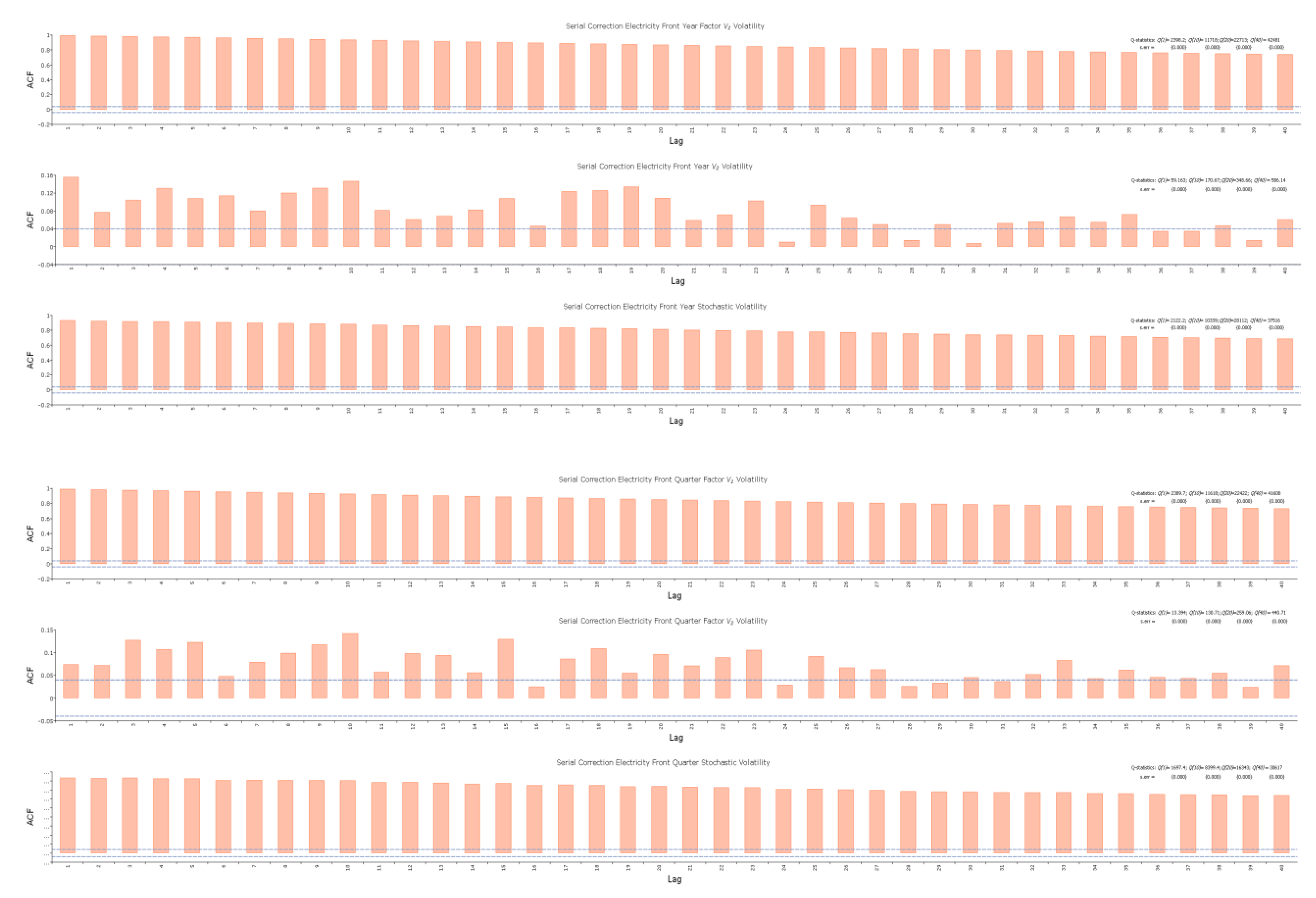
| 0.51887 | 0.48874 | 1.0954 | 2.43301 | 0.13542 | 10.8320 | 9.8053 | 63.85624 | 22713 |
| 0.14465 | 0.0225 | 1.13207 | 0.14916 | {0.0044} | {0.0000} | {0.0000} | {0.0000} | |
| BDS-Z-statistic (e = 1) | Phillips- | Augment | Breusch-Godfrey LM | |||||
| m = 2 | m = 3 | m = 4 | m = 5 | m = 6 | Perron test | DF-test | 10 lags | 20 lags |
| 124.121 | 146.201 | 175.798 | 218.816 | 280.884 | −3.41164 | −3.1497 | 2397.20 | 2397.31 |
| 0.00000 | {0.0000} | {0.0000} | {0.0000} | {0.0000} | {0.0107} | {0.0232} | {0.0000} | {0.0000} |
| Volatility Factor V2 | ||||||||
| Mean (all)/ | Median | Maximum/ | Moment | Quantile | Quantile | Cramer- | Andersen | Serial dep. |
| Mode | Std.dev. | Minimum | Kurt/Skew | Kurt/Skew | Normal | von-Mises | Darling | Q(12) |
| −0.00272 | −0.01341 | 0.3881 | 17.62417 | 0.08493 | 14.3653 | 33.1623 | 181.8012 | 374.23 |
| 0.03744 | −0.0794 | 3.35739 | 0.18380 | {0.0008} | {0.0000} | {0.0000} | {0.0000} | |
| BDS-Z-statistic (e = 1) | Phillips - | Augment | Breusch-Godfrey LM | |||||
| m = 2 | m = 3 | m = 4 | m = 5 | m = 6 | Perron test | DF-test | 10 lags | 20 lags |
| 12.395 | 13.329 | 14.954 | 16.204 | 17.577 | −51.840 | −9.6462 | 180.953 | 224.657 |
| 0.00000 | {0.0000} | {0.0000} | {0.0000} | {0.0000} | {0.0001} | {0.0000} | {0.0000} | {0.0000} |
| Reprojected Volatility (exp(V1 + V2)) | ||||||||
| Mean (all)/ | Median | Maximum/ | Moment | Quantile | Quantile | Cramer- | Andersen | Serial dep. |
| Mode | Std.dev. | Minimum | Kurt/Skew | Kurt/Skew | Normal | von-Mises | Darling | Q(12) |
| 20.61478 | 20.20185 | 31.1449 | 4.29946 | 0.14271 | 11.0575 | 13.8382 | 84.6297 | 20112 |
| 1.71739 | 16.1142 | 1.66877 | 0.14933 | {0.0040} | {0.0000} | {0.0000} | {0.0000} | |
| BDS-Z-statistic (e = 1) | Phillips- | Augment | Breusch-Godfrey LM | |||||
| m = 2 | m = 3 | m = 4 | m = 5 | m = 6 | Perron test | DF-test | 10 lags | 20 lags |
| 86.772 | 99.537 | 115.601 | 137.650 | 168.371 | −8.73293 | −3.1274 | 2202.33 | 2205.25 |
| 0.00000 | {0.0000} | {0.0000} | {0.0000} | {0.0000} | {0.0000} | {0.0247} | {0.0000} | {0.0000} |
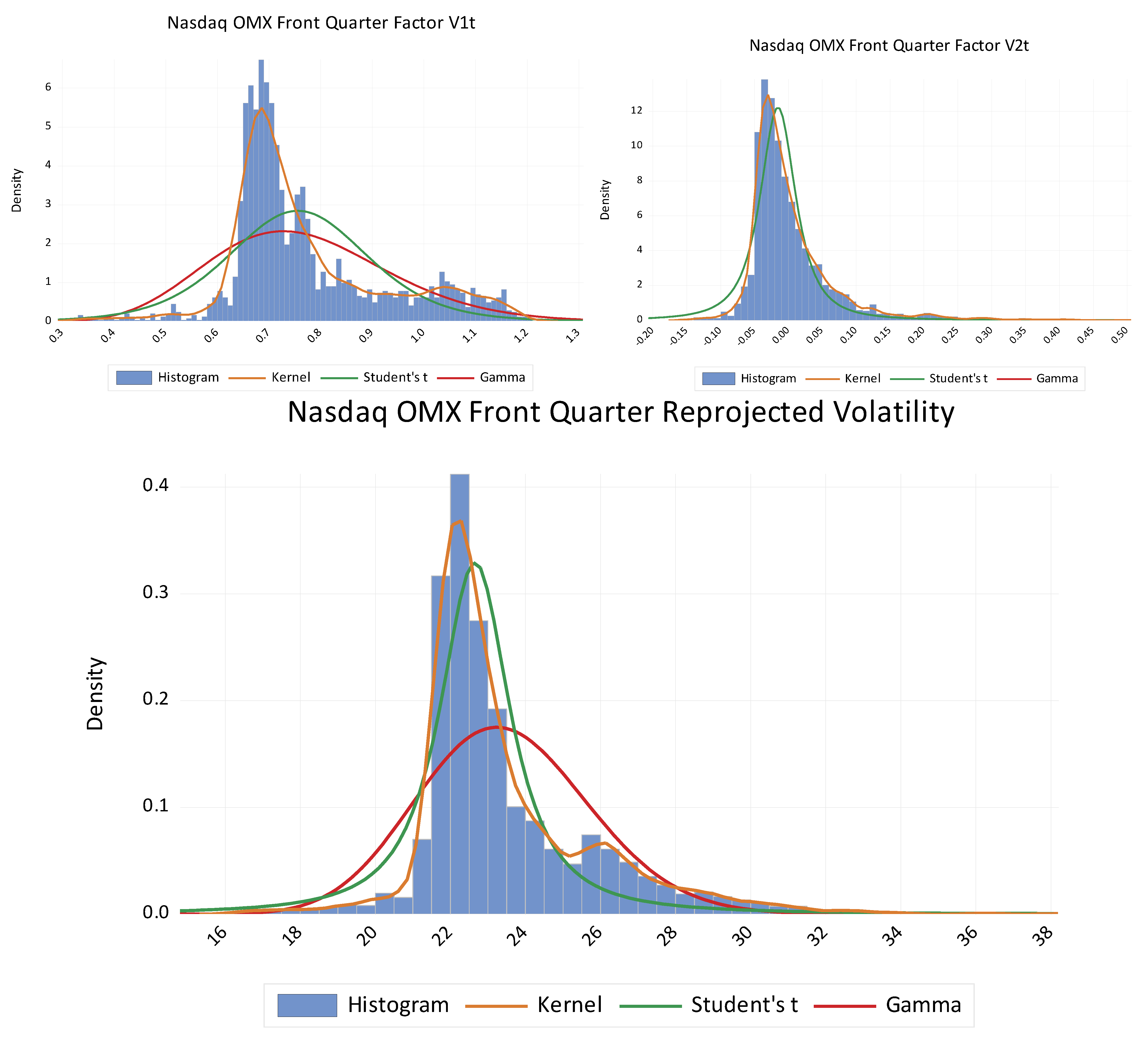
| Panel B | Characteristics Nasdaq Front Quarter Contracts | |||||||
| Volatility Factor V1 | ||||||||
| Mean (all)/ | Median | Maximum/ | Moment | Quantile | Quantile | Cramer- | Andersen | Serial dep. |
| M (-drop) | Std.dev. | Minimum | Kurt/Skew | Kurt/Skew | Normal | von-Mises | Darling | Q(12) |
| 0.76788 | 0.71704 | 1.20739 | 1.56322 | 0.53077 | 122.3606 | 19.5508 | 104.339 | 26513 |
| 0.16247 | 0.02150 | 0.33583 | 0.48238 | {0.0000} | {0.0000} | {0.0000} | {0.0000} | |
| BDS-Z-statistic (e = 1) | Phillips- | Augment | Breusch-Godfrey LM | |||||
| m = 2 | m = 3 | m = 4 | m = 5 | m = 6 | Perron test | DF-test | 10 lags | 20 lags |
| 108.216 | 127.281 | 152.794 | 189.844 | 243.259 | −4.15052 | −4.2901 | 2390.69 | 2390.84 |
| {0.0000} | {0.0000} | {0.0000} | {0.0000} | {0.0000} | {0.0008} | {0.0005} | {0.0000} | {0.0000} |
| Volatility Factor V2 | ||||||||
| Mean (all)/ | Median | Maximum/ | Moment | Quantile | Quantile | Cramer- | Andersen | Serial dep. |
| M (-drop) | Std.dev. | Minimum | Kurt/Skew | Kurt/Skew | Normal | von-Mises | Darling | Q(12) |
| 0.00393 | −0.01455 | 0.56434 | 12.78224 | 0.20480 | 34.3745 | 26.4854 | 146.889 | 290.69 |
| 0.06761 | −0.15333 | 2.83930 | 0.27326 | {0.0000} | {0.0000} | {0.0000} | {0.0000} | |
| BDS-Z-statistic (e = 1) | Phillips - | Augment | Breusch-Godfrey LM | |||||
| m = 2 | m = 3 | m = 4 | m = 5 | m = 6 | Perron test | DF-test | 10 lags | 20 lags |
| 12.4713 | 16.0226 | 18.1589 | 20.1589 | 22.4214 | −55.20717 | −9.8673 | 154.1516 | 190.1991 |
| {0.0000} | {0.0000} | {0.0000} | {0.0000} | {0.0000} | {0.0001} | {0.0000} | {0.0000} | {0.0000} |
| Stochastic Yearly Volatility (√252*exp(V1 + V2)) | ||||||||
| Mean (all)/ | Median | Maximum/ | Moment | Quantile | Quantile | Cramer- | Andersen | Serial dep. |
| M (-drop) | Std.dev. | Minimum | Kurt/Skew | Kurt/Skew | Normal | von-Mises | Darling | Q(12) |
| 23.46186 | 22.72147 | 38.20854 | 3.27852 | 0.36575 | 76.9821 | 22.3128 | 116.342 | 19360 |
| 2.37134 | 16.27464 | 1.40411 | 0.39657 | {0.0000} | {0.0000} | {0.0000} | {0.0000} | |
| BDS-Z-statistic (e = 1) | Phillips- | Augment | Breusch-Godfrey LM | |||||
| m = 2 | m = 3 | m = 4 | m = 5 | m = 6 | Perron test | DF-test | 10 lags | 20 lags |
| 70.6365 | 81.9115 | 95.5908 | 114.165 | 139.986 | −21.88660 | −2.9438 | 1955.24 | 1959.39 |
| {0.0000} | {0.0000} | {0.0000} | {0.0000} | {0.0000} | {0.0000} | {0.0406} | {0.0000} | {0.0000} |
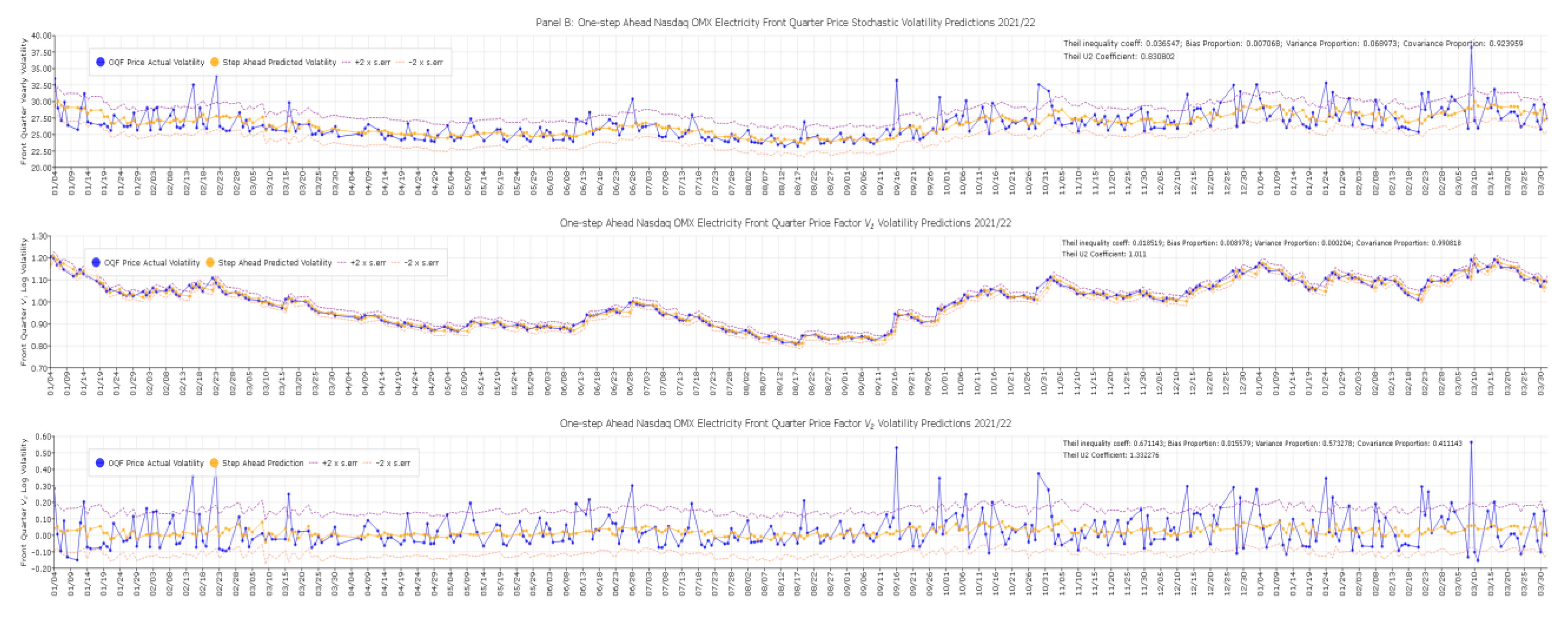
| Estimated Daily Stochastic Volatility Forecast Fit Measures 01/21–04/22: | |||||||
|---|---|---|---|---|---|---|---|
| Factor 1 | Factor 2 | Stochastic | |||||
| Contracts: | Error Measures: | V1t: | V2t: | Volatility (e(V1+V2)): | |||
| Root Mean Square Error (RMSE) | 0.01680 | 0.05883 | 0.89793 | ||||
| Mean absolute Error (MAE) | 0.01240 | 0.03891 | 0.621243 | ||||
| Mean absolute percent error (MAPE) | 1.58480 | 216.2324 | 2.55794 | ||||
| Teil inequality coefficient (U1) | 0.01088 | 0.74757 | 0.01916 | ||||
| Front Year | Bias proportion |  |  |  | |||
| 0.00022 | 0.00196 | 0.02857 | |||||
| Contracts: | Variance Proportion | 0.00330 | 0.53616 | 0.02857 | |||
| Covariance Proportion | 0.99648 | 0.46189 | 0.97119 | ||||
| Theil U2 Coefficient | 0.96810 | 1.67533 | 0.85152 | ||||
| Symmetric MAPE | 1.59258 | 148.6957 | 2.57765 | ||||
| Root Mean Square Error (RMSE) | 0.01739 | 0.10837 | 1.77203 | ||||
| Mean absolute Error (MAE) | 0.01306 | 0.07922 | 1.27864 | ||||
| Mean absolute percent error (MAPE) | 1.27670 | 153.421 | 4.60947 | ||||
| Teil inequality coefficient (U1) | 0.00866 | 0.74741 | 0.03320 | ||||
| Front Quarter | Bias proportion |  |  |  | |||
| 0.00050 | 0.00456 | 0.00051 | |||||
| Contracts: | Variance Proportion | 0.00041 | 0.59765 | 0.14362 | |||
| Covariance Proportion | 0.99909 | 0.39779 | 0.85587 | ||||
| Theil U2 Coefficient | 0.98607 | 1.14376 | 0.76472 | ||||
| Symmetric MAPE | 1.28205 | 151.934 | 4.66220 | ||||
Publisher’s Note: MDPI stays neutral with regard to jurisdictional claims in published maps and institutional affiliations. |
© 2022 by the author. Licensee MDPI, Basel, Switzerland. This article is an open access article distributed under the terms and conditions of the Creative Commons Attribution (CC BY) license (https://creativecommons.org/licenses/by/4.0/).
Share and Cite
Solibakke, P.B. Projecting and Forecasting the Latent Volatility for the Nasdaq OMX Nordic/Baltic Financial Electricity Market Applying Stochastic Volatility Market Characteristics. Energies 2022, 15, 3839. https://doi.org/10.3390/en15103839
Solibakke PB. Projecting and Forecasting the Latent Volatility for the Nasdaq OMX Nordic/Baltic Financial Electricity Market Applying Stochastic Volatility Market Characteristics. Energies. 2022; 15(10):3839. https://doi.org/10.3390/en15103839
Chicago/Turabian StyleSolibakke, Per Bjarte. 2022. "Projecting and Forecasting the Latent Volatility for the Nasdaq OMX Nordic/Baltic Financial Electricity Market Applying Stochastic Volatility Market Characteristics" Energies 15, no. 10: 3839. https://doi.org/10.3390/en15103839
APA StyleSolibakke, P. B. (2022). Projecting and Forecasting the Latent Volatility for the Nasdaq OMX Nordic/Baltic Financial Electricity Market Applying Stochastic Volatility Market Characteristics. Energies, 15(10), 3839. https://doi.org/10.3390/en15103839