Article

Design of a Thermoelectric Device for Power Generation through Waste Heat Recovery from Marine Internal Combustion Engines

by
Georgios Konstantinou
*,
Theodora Kyratsi
and
Loucas S. Louca
Department of Mechanical and Manufacturing Engineering, University of Cyprus, Nicosia 1678, Cyprus
*
Author to whom correspondence should be addressed.
Energies 2022, 15(11), 4075; https://doi.org/10.3390/en15114075
Submission received: 30 April 2022 / Revised: 25 May 2022 / Accepted: 27 May 2022 / Published: 1 June 2022
(This article belongs to the Special Issue Waste Heat Recovery Using Thermoelectric Generators)

Abstract

:
Modern ships discharge large amounts of energy into the environment. More specifically, internal combustion engines (ICE) of commercial and passenger ships waste significant amounts of thermal energy at high temperature through their exhaust gases that are discharged to the atmosphere. A practical approach of recovering some amount of this energy is by using thermoelectric generator systems, which can convert thermal into electrical energy, given that there is a significant temperature difference. It is the aim of this work to propose a thermoelectric generator to recover energy from the exhaust gases of marine ICEs. The proposed thermoelectric generator uses the outside surface of the ICE manifold as the hot side of the thermoelectric module, while the cold side is maintained at a low temperature through a heat sink and induced water flow. The goal of this work is to design this thermoelectric generator and identify the configuration that produces the maximum electric power. The analysis and design are performed with the use of modeling and simulation, while commercial software is employed to study the 3-dimensional coupled fluid flow and heat transfer at a steady state. A sensitivity analysis is carried out to identify the parameters with the highest influence on power production. In addition to a full factorial sensitivity analysis, the more efficient Latin hypercube sampling is used. The analysis shows that significant energy of the exhaust gases can be converted into electric power with the use of an optimized heatsink, which creates the highest temperature difference between the two sides of the thermoelectric module.

1. Introduction

Global warming is evolving into one of the significant problems that humanity is called to battle. One of the major contributors to global warming is the energy and CO2 released into the environment by different sectors of modern industries [1,2]. The scientific community is motivated to study alternative methods to reduce the amount of waste heat energy that industries are currently producing. Each year, modern ships through their internal combustion engines (ICE) discharge massive energy and carbon emissions to the environment. According to the International Maritime Organization (IMO), carbon emissions have increased 8.4% from 2012 to 2019 [3]. In addition, maritime shipping from 2007 to 2012 has accounted for about 2.8% of worldwide greenhouse gases, for both domestic and international operations.
The use of thermoelectric generators (TEG) can provide a solution to convert such waste heat into useful electrical energy. One commercial approach was developed by KELK Ltd. that tested a thermoelectric generation system at a carburizing furnace [4]. Residual carburizing gas heated up the hot side of multiple TEG units, which consisted of 16 Bi-Te modules each. The operating conditions resulted in varying hot side temperatures from 50 to 250 °C and on the other hand, the cold side temperature was kept constant at 30 °C. The results showed that 214 W of electric power was generated, which was used to charge batteries and to power LED lights. Researchers in another work investigated the use of thermoelectric generation systems in a steel production plant. Their TEG included 16 thermoelectric modules made of bismuth-telluride and used radiant heat from hot steel products during continuous casting. The thermoelectric system generated more than 250 W when the hot-side temperature was 250 °C and the cold-side was 30 °C [5]. This system has scaled up to produce up to 9 kW of electric power with the produced steel at 915 °C. A similar solution was introduced in the Portland cement industry, where waste energy is lost into the atmosphere through the outer shell of the rotary kiln. In this work, the system was built as a circular array of TEG units placed at a small distance around the rotary kiln [6]. This system generated about 210 kW, which accounts for about 33% of the energy that could be lost through the kiln surface without the TEG.
In the maritime industry, around 50% of the available fuel energy used to power the diesel ICEs is wasted into the environment [7]. Even though this a significant amount of wasted energy, its quality is low due to the low temperature that this energy is wasted, which in turn results in low recovery efficiency. In addition, this work provides an overview of different waste heat recovery technologies, such as the organic Rankine cycle, Rankine cycle, supercritical Rankine cycle, Kalina cycle and exhaust gas turbine systems. Specifically, waste energy recovery systems from marine incinerators using thermoelectrics have been shown to be a promising option [8,9,10]. Moreover, these works showed that the proposed TEG solution could be financially viable. In another work, the efficiency of the TEG (ZT value) is studied and it was concluded that ZT values higher than 1.5 are more promising, making it a more attractive solution for investment by ship owners [11].
The techno-economic aspects of thermoelectric devices for waste heat energy recovery are also important. For applications with a power output under 10 kW, such as the waste energy of marine ICE, thermoelectric devices can provide a worthwhile solution as they have better efficiency than the Rankine cycle and lower cost [12]. With the future commercial developments of TEGs, they can provide even greater efficiencies in an increased power range of applications.
The use of thermoelectric generators in ICE has numerus advantages. They are solid structures with no moving parts, and they require a small space for installation in addition to their low weight. Compared to other devices, TEGs need only thermal energy to produce electricity, require minimum maintenance and have a long service life. In addition, they can operate in remote locations with no required electricity and can be installed at any location or orientation. The economic changes during these years, high fuel prices and environmental pollution gave the opportunity for more research on environmentally friendly technologies in the marine industry and ship transportations. The ICE generates important waste heat energy through its exhaust gases at high temperature. An efficient way to recover the waste energy from exhaust gases is with the use of thermoelectric generators, which can convert waste heat into electrical energy.
The goal of this work is to design a TEG system that produces the maximum possible power using the exhaust gases of a maritime ICE. First, the description of thermoelectric modules, finite element method and the Latin hypercube sampling approach are given in the Background. Then, the new design, simulation model, and evaluation procedure are given in the Device and Modeling section. Next, the parametric analyses are presented, and finally, conclusions are given.

2. Background

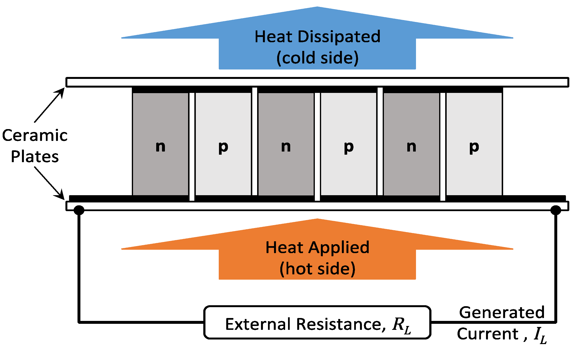
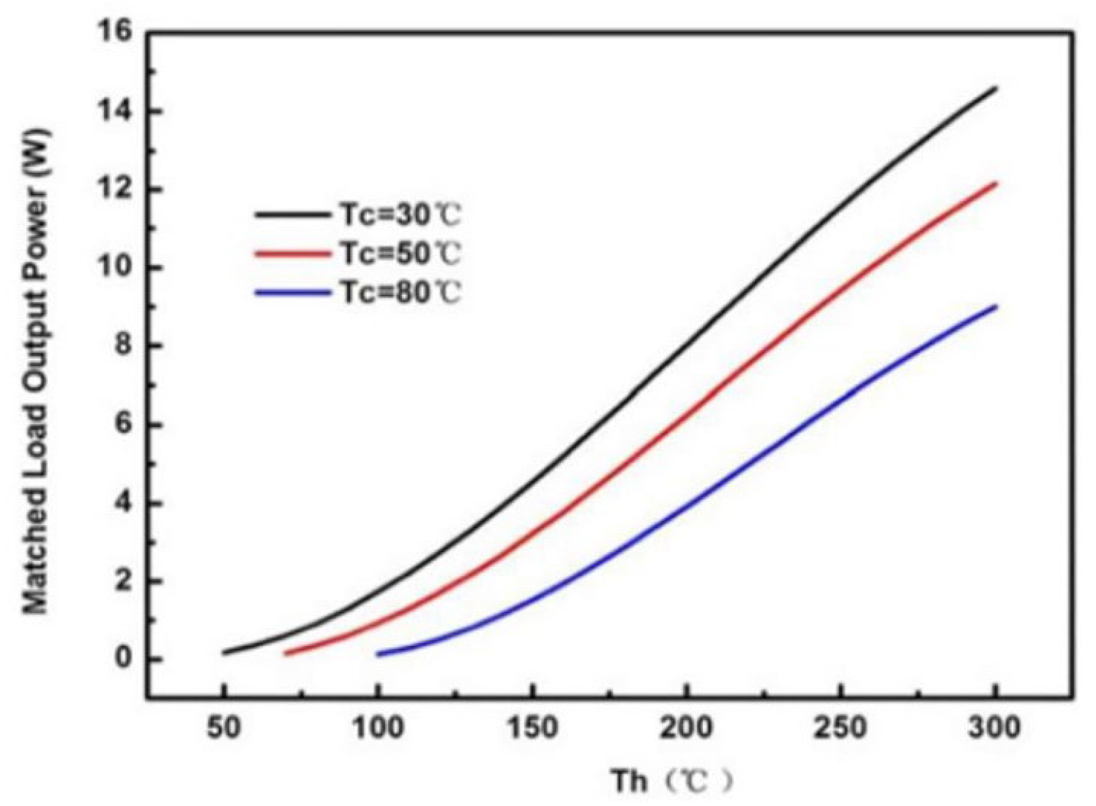
2.1. Thermoelectric Modules

TEG modules operate in two modes, power generation and heat pumping. The Seebeck thermoelectric effect is exploited in this work, which results in the TEG module to operate in power generation mode. By generating a temperature gradient across the two sides of the thermoelectric module, an electrical current is produced. The TEG module contains several thermoelectric n-type and p-type paired legs that are built of highly doped semiconducting materials [13,14]. The electrical connection of the legs is in series in order to increase the voltage; however, the two sides of all legs have the same temperature (thermally connected in parallel). The legs are enclosed between two ceramic plates for electrical insulation (Figure 1).
The p-type legs are positively charged due to the lack of electrons and a current flow is created when a heat flow exists. Heat and current flow have the same direction. On the contrary, n-type legs have a negative charge so current and heat are counter flowing. Due to the series connection, the voltage produced by each pair is added to create the overall module voltage. The power that a thermoelectric generator produces is capable of powering standard electrical or electronic devices. Modules of bismuth telluride (Bi2Te3) are considered in this work. The physical properties used in the simulations and power calculations are given in Table 1. The parameters in this table are only the ones necessary for the thermal analysis of the TEG device, and they are assumed constant. In general, these parameters are dependent on temperature but their change is insignificant for the temperature range used in this work. The dimensions of the module are 50 × 50 × 4 mm and produces maximum power when applying the temperatures provided by the manufacturer (30 °C and 300 °C). This TEG module is selected due to its compatibility to the temperature difference of the specific implementation as it is going to be described later. The power curves for this TEG module for various cold and hot temperatures are given in Figure 2. These power data are provided by the manufacturer [15] and contain the thermoelectric material properties, such as the ZT and Seebeck coefficient.

2.2. Finite Element Method and Solvers

The finite element method (FEM) will be used to solve the partial differential equations that describe the behavior of the model. With FEM, the complex and nonlinear differential equations can be solved for the non-canonical geometries of the domains of interest. For this work, the commercial software COMSOL Multiphysics is used [16,17]. For this model, an implementation between the heat transfer differential equations and the laminar flow differential equations will be used.
The equations for the heat transfer are solved by the FEM for the entire computational volume. The general differential equations are presented in Equations (1) and (2) and their solution determines the temperature, T, and heat flux, q . The required parameters to solve the equations are the density of the fluid and solid density ρ, specific heat capacity for solid and fluid material Cp, thermal conductivity for solid and fluids k. In addition, the velocity field that is defined by the coupling with the stationary incompressible laminar flow is needed. For this work, the differential equations are used in a stationary form, where the time dependent terms are eliminated from the equation. Equation (2) describes the relationship of heat flux with the temperature gradient. In this work, this relationship is crucial due to the non-symmetrical tensor that this equation provides.
ρ C p u · T + · q = Q
q = k T
The solution of Equations (1) and (2) requires the definition of the appropriate boundary conditions. For the analysis in this work, two different forms of boundary conditions are used. On surfaces with thermal insulation, the heat flux is zero, and this condition is expressed by Equation (3). Moreover, on surfaces with interaction between the ambient air and the device, there is heat transfer by means of convection and this heat flux is expressed by Equation (4). In these equations, h is the convection coefficient, n is the unit vector normal to the outside surfaces, and T a m b is the ambient temperature.
n · ( k T ) = 0
n · ( k T ) = h · ( T a m b T )
The COMSOL software has a variety of FEM solvers that can be used for the simulation with Multiphysics phenomena and interactions. The use of each solver depends on the convergence of the model and the available processing power. Different types of solvers have been used to evaluate the computational time and convergence. In this work, the solver that is chosen is the segregated solver with Parallel sparse Direct Solver (PARDISO) [18]. PARDISO is one of the best methods to solve large mesh problems faster because in large scale simulations with nodes that are zero, sparse matrix algorithms can reduce the computational time from the fact that in their matrices, they do not include the zero nodes in data storage.

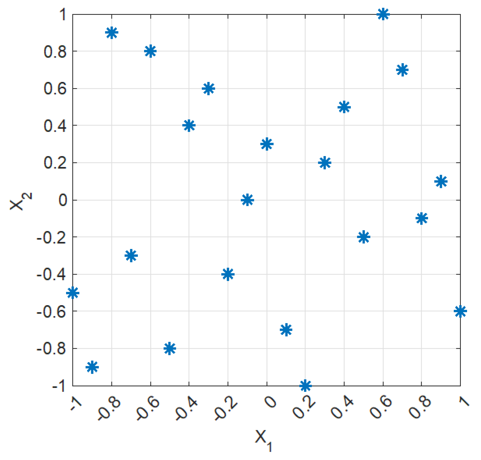
2.3. Latin Hypercube

Generally Latin Hypercube Sampling (LHS) is a method that attempts to allocate random numbers evenly over a multidimensional parameter space [19,20]. The advantage of this method over an ordinary random sampling is that the LHS can distribute the parameters evenly around the center of the parameter space. This is particularly beneficial when large number of parameters need to be evaluated and/or time-consuming computations are required for evaluating the performance of each parameter set. The LHS approach enables uniform coverage of the design space while limiting the number of the parameter set points to a minimum, which in turn reduces evaluation time. An example of a two-dimensional LHS with twenty-one points is shown in Figure 3, where each ‘∗’ represents a point of the parameter set. Note the uniform coverage of the two-dimensional space with at least one point for each value of X1 and X2 (column and row). Covering the same space with a full factorial approach would require 212 = 441 points. Moreover, an advantage of LHS is the flexibility that it provides. In this case, if one of the set of parameters must be eliminated from the study due to geometric limitations, the existing data can still be used without a reduction in the evaluation points. In this study, the use of LHS can help determine the area of interest and allow the examination of a larger range of values.

3. Device and Modeling

Generally, the waste heat from the ICE comes from exhaust gases at high temperature. As a result, the available positions for the TEG device to operate is after the combustion chamber. The exhaust gases for a typical 7-cylinder ICE with engine power 7 to 12 MW are used and the temperature of the exhaust gases is around 370 °C. This turbocharged engine series operates in typical commercial ships and its overall power depends on the number of cylinders (5 to 8), rotational speed (95–124 RPM) and engine configuration. It has a 500 mm bore, 2010 mm stroke and a length of 7.34 m for 7 pistons.
There are different available positions that the TEG can be installed, such as the cylinder exhaust port, engine bypass system, engine manifold, and ship chimney. For this study, the manifold is chosen because the manifold had two circular flat surfaces at its ends as shown in Figure 4. Other installation positions are possible and can be explored using the procedure developed in this paper. However, the manifold position is chosen since it is the least intrusive to the ICE system, which leads to simpler modifications for the installation. Taking into consideration the exhaust gases temperature and the temperature losses, a conservative approach is used and the temperature on the outside surface of the manifold is set to be 270 °C, where the hot side of the TEG will be installed.

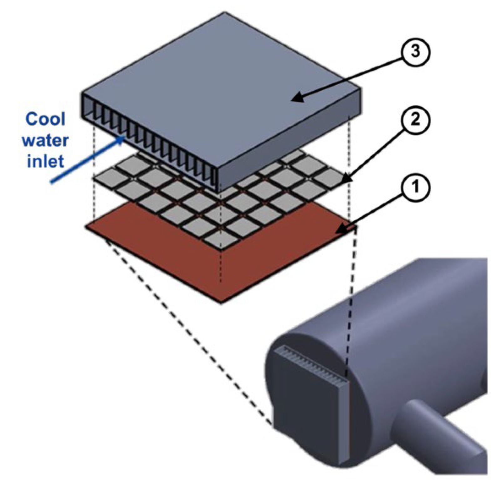
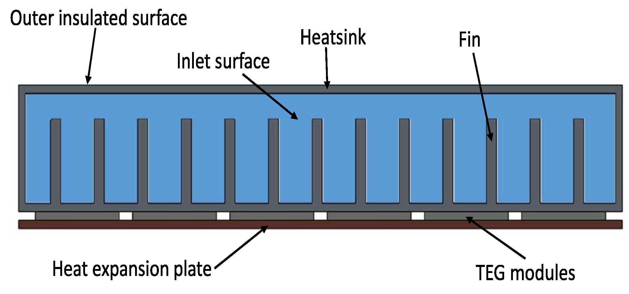
3.1. Thermoelectric Device

The proposed thermoelectric device consists of the following three main parts: the heat expansion plate (1), thermoelectric modules (2), and the water cooled heatsink (3), as shown in Figure 5. The area between the TEG modules is assumed to be static air. To achieve a high temperature difference between the hot and the cold side of the modules, the modules are sandwiched between the cooling heatsink and the heat expansion plate. The expansion is in direct contact with the outside surface of the manifold. The device has a square profile, its overall dimensions are 360 × 360 mm and it includes a total of 36 modules arranged in a 6 × 6 pattern. These dimensions allow for an 8 mm gap between the modules and a 10 mm empty space at each end. These gaps are necessary for electrical connections and cables that run from each module to the outside connections of the TEG.
The cooling heatsink is an enclosed rectangular tube that allows the flow of the water in order to extract heat and create a low temperature on the cold side of the modules. The lower surface of the heatsink is in contact with the modules. The inside area of the heatsink includes longitudinal fins that increase the overall heat transfer area and, therefore, the heat transferred from the modules to the water. The configuration of the heatsink is shown in Figure 6. The fins can have a variable height and width that will be determined later using the parametric studies. In addition, the number of fins or gap between the fins is variable. Initially, the heatsink has an overall height of 60 mm and 15 fins.

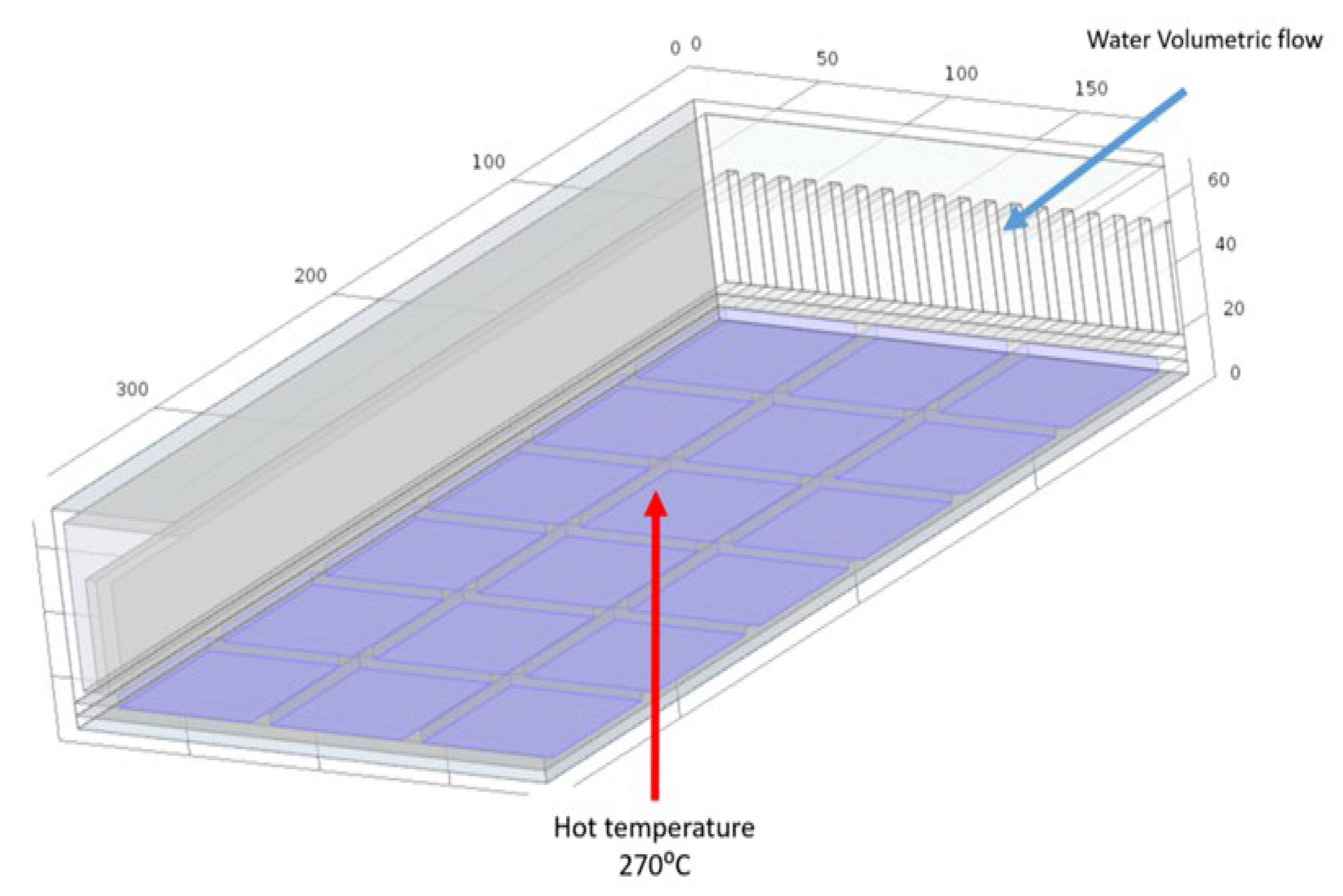
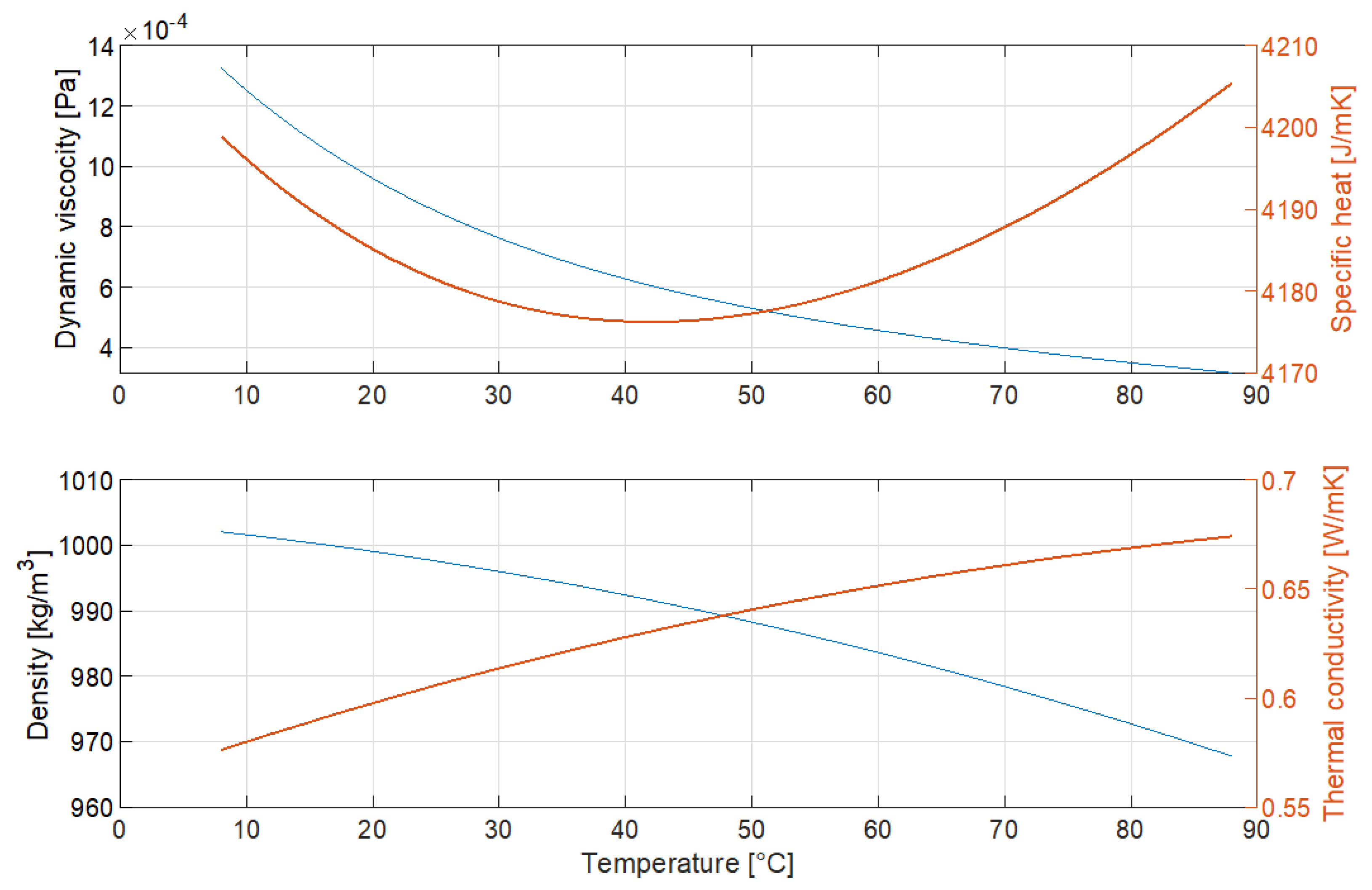
3.2. Modeling and Analysis

The geometry of the model is designed inside the COMSOL software using a set of parameters that describe each characteristic of the model geometry. The exact model geometry is defined by the following three parameters of the fins: number, thickness, and height. Note that by varying these parameters, the inlet velocity is changed due to the change in inlet surface. These parameters will be later varied by the parametric studies in order to identify the most sensitive parameters to the produced net electric power.
The TEG device model, with its three-dimensional geometry, includes non-isothermal flow with laminal incompressible flow conditions and conjugate heat transfer at the interface between the fluid and the heatsink. These Multiphysics model behaviors and interactions are described by the partial differential equations described above. A vital part of the model is the boundary conditions, as shown in Figure 7. For the heat transfer, the inlet temperature is set to a constant 20 °C and for the outlet is set to “outflow” that enforces heat transfer only by convection. The outer surface of the heat expansion plate is set to be 270 °C, which is the temperature of the manifold. The outside surface of the device is assumed adiabatic, due to the insulation of the manifold enclosure for safety reasons. For the flow, the inlet surface boundary condition is set to constant velocity, where the outlet surface is set to constant pressure (atmospheric). The inlet water velocity is determined by the volumetric flow that is kept constant 0.4 L/s, i.e., the velocity changes due to the different inlet surface for each set of fin parameters. This assumption ensures that the cooling capacity is constant; therefore, only the effect of the heatsink parameters will be accounted for the different designs.
The material physical properties are also required to perform the simulation. The material properties for the heatsink (aluminum) and heat expansion plate (cooper) are given in Table 2. These properties are assumed constant and to not change with temperature, which is a suitable assumption for solids. On the other hand, fluid physical properties are not constant and can be temperature dependent for both the air and the water. For water, the temperature dependency for thermal conductivity, heat capacity, dynamic viscocity, and density is used and shown in Figure 8. The air in the gap between the modules is considered static (solid), since it is not moving. Therefore, only thermal conductivity and specific heat transfer are needed, and their temperature dependency is shown in Figure 9.
To take into consideration the velocity changes for different geometries during the parametric study, the velocity for each parameter set is calculated considering a constant volumetric flow. Model geometry for a given parameter set value is calculated through the formulas given in Table 3. This type of geometric model setup allows the easy implementation of paremetric studies without constant supervision of COMSOL or having to run each simulation separately.
Before using the FEM model for the analysis, its accuracy is considered. At first, a mesh convergence study is performed with the use of different mesh sizes and types in order to identify the proper mesh for the model and the most effective mesh in terms of computational time. Another important factor is the validation of the FEM models with analytical models when possible. For this work, a 1D thermal resistance model, along the height of the heatsink, is used to validate the results from the FEM model. This validation study shows that the 1D model predicts temperatures that are very close to the COMSOL model results, as it is depicted in Figure 10.
To identify the final model geometry and parameters, general studies are performed to identify the model that will be later used for the full factorial parametric and Latin hypercube studies. Initially, a model with an inlet and outlet volume that acts as a manifold before and after the fins is studied. This is what one would expect in the actual device in order to distribute the constant water volumetric flow, but also for easy manufacturing. In contrast, this study shows that this added volume increases rapidly the number of mesh elements, due to the complex geometry at the beginning and ending of the fins. This larger mesh size results in a significant increase in computational time without significant changes in the predicted temperature profiles. As a result, the inflow and outflow volume are eliminated. Another study considered the height of the fins. Having fins that do not cover the whole height of the heatsink and having a gap at the top do not create lower temperatures at the cold side of the module, and in addition, it increases the computational cost due to more complex flow. The simulation results show that the fins should cover the entire height of the heatsink. As a result, small rectangular channels form across the width of the TEG device and the final geometry is shown in Figure 11. In addition, the effect of each heatsink parameter on the temperature is studied. This analysis showed that the three most significant parameters are the height of the heatsink, the thickness and number of the fins inside the heatsink.
Finally, the computational efficiency is considered given that the FEM has about 4 million elements. This model has a simulation time of about 1 h; therefore, the model geometry symmetry is exploited to reduce the computation time. The geometry is symmetric around a vertical plane in the middle of the heatsink and this defined in COMSOL. This results in a model about half the size of the original, which can be computed in about 32 min on an 8 core processor at 4 GHz and 128 GB of RAM.
For the calculation of the net power, the surface temperatures of the cold and hot sides of the modules are exported from COMSOL. A typical temperature profile of the cold side within COMSOL is shown in Figure 12. The cooling water enters the heatsink at the left side (x = 0). As it can be observed in the right plot with the mesh, the available temperatures are at the nodes of the mesh that do not necessary align with the respective temperatures of the module at the hot side. The temperature at the hot side is not very interesting, since it remains almost constant with about 0.4 °C variation. The exported temperatures are imported into MATLAB for analyzing. First, the available temperature points are linearly interpolated in order to get the temperature at the same points for the cold and hot side, as shown in Figure 13. This is critical for the accurate calculation of the power. The power is then calculate using the module data presented in the Background section. The next step is to calculate the pressure drop through analytical expressions and the overall power losses required to maintain the flow used in the simulation. This power is subtracted from the module power to calculate the net power. For the module power calculation, the modules are divided into smaller cells and the power for each cell is shown in Figure 14. The produced power is the sum of the individual power of all these cells.

4. Parametric Studies

The parametric studies are performed in order to evaluate the effect of a variety of possible combinations of the device parameters. Based on the study performed in the previous section, it was determined that only the geometric parameters of the heatsink effect the power production significantly. More specifically, the number and thickness of fins and the heatsink height were considered. A variety of methodologies are available for performing parametric studies and for the purposes of this work, two were employed, i.e., full factorial and Latin hypercube sampling.

4.1. Full Factorial

The parametric analysis using the full factorial approach can be lengthy, since it exponentially increases with the number of parameters and the number of points per parameter. A high number of evaluations are required to identify the finest set of parameters. In this case, we have only three parameters, so this approach is workable if a small number of points per parameter in used. Three points per parameter are selected, which gives a total 33 = 27 analyses. The parameter values are shown in Table 4. These specific values are selected in order to avoid the possibility of having a negative channel thickness, which creates a non-real model that cannot be simulated.
The main goal of the full factorial parametric study is to identify the parameters with the highest contribution to energy recovery. This is achieved with the evaluation of the different set of parameters. The produced power without and with the power loss needed to create the necessary water flow are calculated and the results are shown in Figure 15. The calculations confirm the impact of power losses for creating the required water flow. The maximum gross power produced appears at point 25, with parameter values 7, 30 and 45; however, after removing the flow losses, the maximum net power appears at point 26 with parameter values 7, 45 45. The higher water velocity (smaller channel area) at point 25 creates significant power losses that overcome the higher produced power as compared to point 26. In general, the last three points have the highest power losses because of the highest number of fins and smallest channel area. In addition, this demonstrates that the temperature difference cannot be an optimization parameter by itself due to the importance of power losses. The maximum net power is 367.8 W and the respective geometric parameters are 7 mm fin thickness, 45 mm heatsink height, and 45 fins.

4.2. Latin Hypercube Sampling

As mentioned before, the LHS method can better cover the same parameter space with the same number of evaluation points. The LHS parameter sets are generated using the MATLAB toolbox and they also are checked for not exceeding the geometric constraints. A total of 46 parameter set points are created and they are shown in the Appendix A. The number of fins is constraint to an odd integer number due to an unimportant model geometric limitation. These parameter set points are imported into COMSOL and simulated to produce the temperature distribution for each parameter set. The simulation results are then exported to MATLAB to calculate the produced power. The results of the LHS parametric study are shown in Figure 16. The LHS parametric study provides a new maximum power of 368.3 W, which is produced by parameter set 10. The geometric parameters for producing this power are 6 mm fin thickness, 44 mm heatsink height, and 49 fins. As expected, LHS was able to identify a better design as compared to the full factorial analysis.

5. Conclusions

Significant exhaust gases energy from maritime ICE engines can be recovered and converted into electricity with the use of a properly designed thermoelectric generator system. This design, noted as the “best”, is identified using systematic design methodology and Latin hypercube sampling. More specifically, an optimized heatsink for providing the lowest possible temperature at the cold side of the thermoelctric module is designed. The design analyses are made possible by modeling and simulation that provide the required temperature distribution at the two sides of the thermoelctric modules. The proper and methodical building of the FEM model allows efficient simulation that, in turn, enables the investigation of the multible designs in a short time.
The developed model will be used in future studies for further exploration of the design space by studying the effect of other device parameters on the produced power. In this study, only the geometry of the heatsink and its effect on the performance of the device is considered. There are many other device parametres that affect the efficiency and their contribution can be investigated using the proposed approch in this work. For example, different heatsink materials, patterns of thermoelectric modules, size of thermoelectric modules and cooling water flow rate can be examined more efficiently using LHS; however, this remains as future work.

Author Contributions

Conceptualization, L.S.L.; Formal analysis, G.K.; Funding acquisition, T.K.; Investigation, G.K.; Methodology, G.K. and L.S.L.; Project administration, T.K.; Software, G.K.; Supervision, T.K. and L.S.L.; Writing—original draft, G.K., T.K. and L.S.L. All authors have read and agreed to the published version of the manuscript.

Funding

This research was funded from the MarTEnergy Project, funded by the M-ERA.NET 2017–2020 (P2P/M-ERA.Net/0317/0004).

Institutional Review Board Statement

Not applicable.

Informed Consent Statement

Not applicable.

Acknowledgments

The authors acknowledge the support from the MarTEnergy Project, funded by the M-ERA.NET 2017–2020 (P2P/M-ERA.Net/0317/0004). The authors would also like to express their appreciation to Columbia Shipmanagement Ltd. for providing technical information and data regarding this work.

Conflicts of Interest

The authors declare no conflict of interest.

Appendix A. Parameter Sets for Latin Hypercube Sampling

Parameter Set #Fin Thickness [mm]Number of FinsHeatsink Height [mm]Parameter Set #Fin Thickness [mm] Number of FinsHeatsink Height [mm]
1445502425542
2445422524958
3247482623124
4243402743130
5437382845126
6241322944736
7437443024526
8439443124934
9247463225358
10649443324136
11245503443340
12231403544328
13437343643734
14435263723554
15251563843348
16451283944352
17447384064132
18241284143558
19439304225150
20633564343156
21633464424336
22635544563946
23249544623942

References

  1. Ring, M.J.; Lindner, D.; Cross, E.F.; Schlesinger, M.E. Causes of the global warming observed since the 19th century. Atmospheric Clim. Sci. 2012, 2, 401–415. [Google Scholar] [CrossRef] [Green Version]
  2. Hegerl, G.C.; Broennimann, S.; Cowan, T.; Friedman, A.R.; Hawkins, E.; Iles, C.E.; Mueller, W.; Schurer, A.; Undorf, S. Causes of climate change over the historical record. Environ. Res. Lett. 2019, 14, 123006. [Google Scholar] [CrossRef]
  3. International Maritime Organization. Fourth IMO Green House Gas Study; International Maritime Organization: London, UK, 2020. [Google Scholar]
  4. Kaibe, H.; Makino, K.; Kajihara, T.; Fujimoto, S.; Hachiuma, H. Thermoelectric generating system attached to A carburizing furnace at komatsu Ltd., awazu plant. In AIP Conference Proceedings; American Institute of Physics: College Park, MD, USA, 2012; Volume 1449, p. 524. [Google Scholar]
  5. Kuroki, T.; Kabeya, K.; Makino, K.; Kajihara, T.; Kaibe, H.; Hachiuma, H.; Matsuno, H.; Fujibayashi, A. Thermoelectric generation using waste heat in steel works. J. Electron. Mater. 2014, 43, 2405–2410. [Google Scholar] [CrossRef]
  6. Luo, Q.; Li, P.; Cai, L.; Zhou, P.; Tang, D.; Zhai, P.; Zhang, Q. A thermoelectric waste-heat-recovery system for Portland cement rotary kilns. J. Electron. Mater. 2014, 44, 1750–1762. [Google Scholar] [CrossRef]
  7. Singh, D.V.; Pedersen, E. A review of waste heat recovery technologies for maritime applications. Energy Convers. Manag. 2016, 111, 315–328. [Google Scholar] [CrossRef]
  8. Kristiansen, N.R.; Snyder, G.J.; Nielsen, H.K.; Rosendahl, L. Waste heat recovery from a marine waste incinerator using a thermoelectric generator. J. Electron. Mater. 2012, 41, 1024–1029. [Google Scholar] [CrossRef] [Green Version]
  9. Liu, C.; Li, F.; Zhao, C.; Ye, W.; Wang, K.; Dong, Y.; Gao, W. Experimental research of thermal electric power generation from ship incinerator exhaust heat. In IOP Conference Series: Earth and Environmental Science; IOP Publishing: Bristol, UK, 2019; Volume 227, p. 22031. [Google Scholar]
  10. Kristiansen, N.R.; Nielsen, H.K. Potential for usage of thermoelectric generators on ships. J. Electron. Mater. 2010, 39, 1746–1749. [Google Scholar] [CrossRef] [Green Version]
  11. Loupis, M.; Papanikolaou, N.; Prousalidis, J. Fuel consumption reduction in marine power systems through thermoelectric energy recovery. In Proceedings of the 2nd International MARINELIVE Conference on All Electric Ship, Athens, Greece, 12–13 February 2014. [Google Scholar]
  12. Anderson, K.; Brandon, N. Techno-economic analysis of thermoelectrics for waste heat recovery. Energy Sources Part B Econ. Plan. Policy 2019, 14, 147–157. [Google Scholar] [CrossRef]
  13. Lee, J.; Choo, S.; Ju, H.; Hong, J.; Yang, S.E.; Kim, F.; Gu, D.H.; Jang, J.; Kim, G.; Ahn, S.; et al. Doping-induced viscoelasticity in PbTe thermoelectric inks for 3D printing of power-generating tubes. Adv. Energy Mater. 2021, 11, 2100190. [Google Scholar] [CrossRef]
  14. Snyder, Χ.G.J.; Toberer, E.S. Complex thermoelectric materials. Nat. Mater. 2008, 2, 105–114. [Google Scholar] [CrossRef]
  15. TECTEG MFR. Available online: https://thermoelectric-generator.com (accessed on 3 February 2021).
  16. Pryor, R.W. Multiphysics Modeling Using COMSOL: A First Principles Approach; Jones & Bartlett Learning: Sudbury, MA, USA, 2011; ISBN 978-0763779993. [Google Scholar]
  17. COMSOL, Inc. COMSOL Multiphysics Version 5.2 User’s Guide; Comsol Inc.: Burlington, MA, USA, 2017. [Google Scholar]
  18. Schenk, O.; Gärtner, K. Solving unsymmetric sparse systems of linear equations with PARDISO. Future Gener. Comput. Syst. 2004, 20, 475–487. [Google Scholar] [CrossRef]
  19. Viana, F.A.C. A tutorial on latin hypercube design of experiments. Qual. Reliab. Eng. Int. 2015, 32, 1975–1985. [Google Scholar] [CrossRef]
  20. Stein, M. Large sample properties of simulations using latin hypercube sampling. Technometrics 1987, 29, 143. [Google Scholar] [CrossRef]
Figure 1. TEG module configuration.
Energies 15 04075 g001
Figure 2. Power data of TEG module.
Energies 15 04075 g002
Figure 3. LHS−2D space sample.
Energies 15 04075 g003
Figure 4. ICE manifold.
Energies 15 04075 g004
Figure 5. Exploded view of TEG device.
Energies 15 04075 g005
Figure 6. Front view of TEG device.
Energies 15 04075 g006
Figure 7. Model Boundary conditions.
Energies 15 04075 g007
Figure 8. Water thermal properties.
Energies 15 04075 g008
Figure 9. Air thermal properties.
Energies 15 04075 g009
Figure 10. The 1D thermal resistance model vs. COMSOL model.
Energies 15 04075 g010
Figure 11. Final model geometry.
Energies 15 04075 g011
Figure 12. Original cold temperature surface within COMSOL.
Energies 15 04075 g012
Figure 13. Cold side temperature profile after resampling.
Energies 15 04075 g013
Figure 14. Produced power per cell.
Energies 15 04075 g014
Figure 15. Full factorial parametric study results for power with and without losses.
Energies 15 04075 g015
Figure 16. LHS parametric study results.
Energies 15 04075 g016
Table 1. TEG module properties.
ParameterValue
Thermal conductivity k [W/mK]1.2
Density ρ [kg/m3]7700
Specific heat Cp [J/kgK]154
Table 2. Solid material properties.
Material PropertyAluminumCooper
Thermal conductivity k [W/mK]238400
Density ρ [kg/m3]27008960
Specific heat Cp [J/kgK]900385
Table 3. Model geometry.
ParameterCalculation FormulaDescription
h_heatsink60 [mm]Heatsink height
t_fin4 [mm]Fin thickness
n_size30Number of fins
h_finh_heatsink-8 [mm]Fin height
t_chan(352 − n_size × t_fin)/(n_size + 1) [mm]Channel thickness
Entry_area(t_vent × (n_size + 1) × h_fin) [mm2]Inlet area
Q_entry0.0004 [m3/s]Volumetric flow
v_entryQ_entry/Entry_area [m/s]Water velocity
Table 4. Full factorial parameter values.
ParameterValue
Fin thickness3, 5, 7 [mm]
Heatsink height30, 45, 60 [mm]
Number of fins23, 33, 43
Publisher’s Note: MDPI stays neutral with regard to jurisdictional claims in published maps and institutional affiliations.

