Slope Estimation Method of Electric Vehicles Based on Improved Sage–Husa Adaptive Kalman Filter

Abstract

In order to deal with many influence factors of electric vehicles in driving under complex conditions, this paper establishes the system state equation based on the longitudinal dynamics equation of vehicle. Combined with the improved Sage–Husa adaptive Kalman filter algorithm, the road slope estimation model is established. After the driving speed and rough slope observation are input into the slope estimation model, the accurate road slope estimation at the current time can be obtained. The road slope estimation method is compared with the original Sage–Husa adaptive Kalman filter road slope estimation method through three groups of road tests in different slope ranges, and the accuracy and stability advantages of the proposed algorithm in road conditions with large slopes are verified.

1. Introduction

Accurate road slope prediction method is of vital importance in the field of autonomous driving. The system collects parameters through algorithms, predicts the slope at the next moment in advance, and prepares to control the vehicle power system at the next moment, so as to improve the control ability of automatic transmission of vehicles, optimize the power and economy of vehicles, and reduce energy consumption while running smoothly. The parameters of the vehicle the system collects include torque, vehicle speed, acceleration, slope, etc. Among all the parameters, accurate slope information acquisition and prediction has a very special research significance for intelligent vehicle driving; details are shown below.

Figure 1 explains the basic principle of unmanned driving—all behaviors of human drivers in driving can be planned into three steps: environmental perception, decision and planning, control and execution. Environmental perception is the first and most important part. For example, human drivers collect the road condition information of the current vehicle through hearing and vision, and make decisions about the following driving behavior according to this information. Autonomous driving systems also need to collect road information before planning power systems, so high-precision collection algorithms are very important. In addition, the parameter of road slope is a very important part of the longitudinal dynamics equation of the vehicle. Both rolling friction and slope resistance are related to the road slope of the vehicle at the current moment, which to some extent determines the advantages and disadvantages of the adjustment of the dynamic performance of the vehicle in the automatic driving link.

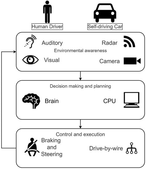
Figure 1. Concept of autonomous driving.

From the perspective of the long-term development of automatic driving, accurate slope prediction is the necessary guarantee for automatic driving technology to step into level 4 and level 5. Level 5 autonomous driving technology requires the vehicle to be able to navigate unknown roads and environments. Therefore, scholars all over the world have done a lot of research on slope prediction and have achieved some results.

In the past 5 years, most of the research on slope estimation algorithms has been based on longitudinal dynamics of vehicles. Some scholars designed a series of slope estimation methods using unscented Kalman filter, such as Dual Unscented Kalman Filter (DUKF) and Quaternion Unscented Kalman Filter (QUKF) [1,2,3,4]. A few scholars used extended Kalman filter to construct slope estimation methods and achieved some results [5,6]. The least square method was also used to construct slope estimation algorithms [7,8,9]. Jiang et al. proposed a two-stage estimation method for vehicle mass and road slope under longitudinal moving condition of mini fuel cell vehicle (FCV) [10]. Hu et al. established the longitudinal kinematics model of vehicles, using the recursive least squares method with adaptive forgetting factors and extended Kalman filter algorithm to estimate the vehicle mass and road grade, respectively [11]. Rodríguez et al. presented a novel accurate estimator based on errorEKF and UKF for vehicle dynamics [12]. Bian et al. presented a MPC based vehicular following control algorithm with road grade prediction [13]. Feng et al. proposed a slope estimation algorithm based on multi-model and multi-data fusion [14].

To sum up, the accuracy of slope prediction is closely related to autonomous driving technology. At the same time, slope estimation is an important cornerstone of the development of autonomous driving technology. Previous literatures have achieved certain results in slope prediction with good prediction accuracy, but there are still gaps in some aspects. The accuracy of the basic Kalman filter has struggled to meet the current requirements of automatic driving. The extended Kalman Filter (EKF) uses Taylor Expansion to construct approximate linear function by obtaining the slope of nonlinear function. The nonlinear system is approximated to linear system by means of ignoring the higher-order term, which inevitably introduces linear error and even leads to the divergence of filter. Thus, the accuracy of slope estimation is reduced. Unscented Kalman filter (UKF) is more accurate than EKF, and its accuracy is equivalent to second-order Taylor expansion, but the speed is slower. A large amount of calculation will require a longer calculation time, so whether it can be applied to the dynamic slope estimation of vehicles remains to be discussed. If the technical choice is to use hardware means to speed up the calculation, the cost of hardware is also higher.

In many Kalman filter algorithms, adaptive Kalman filter plays a very important role. Adaptive Kalman filter uses the measured data to filter and continuously judge whether the system dynamic changes by filtering itself. The model parameters and noise statistics are estimated and modified to improve the filter design and reduce the actual error of the filter. It automatically scales the system noise covariance matrix $Q$. It is considered that the algorithm has fewer tuning parameters and better robustness than the scaling state covariance matrix algorithm [15]. Therefore, scholars have done a lot of research on it. They combined adaptive steps with extended Kalman filter, untraced Kalman filter and other algorithms to derive a series of adaptive Kalman filters, and have made considerable achievements in various fields [16,17,18,19,20,21,22,23]. Due to the addition of adaptive steps, the accuracy of AEKF and AUKF algorithm is improved and the convergence speed is accelerated compared with the original algorithm. However, considering the complexity of calculation of UKF and EKF, on the premise of the same data sets and the same hardware devices, AKF’s calculation speed is higher than AEKF’s, and AEKF’s calculation speed is higher than AUKF’s. Adaptive Kalman filter has also made some contributions to slope estimation. Liao et al. proposed a road slope estimation method based on AEKF [24]. The method was based on the longitudinal dynamics equation of vehicle, and the state space system was discretized. Then, the innovation-based adaptive tuning part was designed to estimate time-varying process noise covariance and measurement noise covariance. Finally, the proposed method was verified by simulation on Carsim platform, and the result was better than the existing EKF algorithm. Sun et al. proposed a road slope estimation method based on AUKF [25]. By increasing the initial noise of the mass prediction model and designing the adaptive shrinkage coefficient to dynamically adjust the covariance matrix of the prediction error, the method realized the rapid and accurate joint estimation of vehicle mass and road slope under the condition of small acceleration. This adaptive step shortened the convergence time of UKF algorithm to some extent, but the convergence time was still about 10 s.

In this paper, an improved road grade estimation method based on Sage–Husa adaptive Kalman filter is proposed. In the method, the model is established based on the longitudinal dynamics of vehicles. The missing quantity in Sage–Husa algorithm is supplemented in the adaptive covariance matrix $Q$, and the updating of prediction noise q and observation noise r is cancelled. The effect of initial noise variance in Sage–Husa algorithm is retained to some extent, and the proportion of fixed noise variance can be controlled. At the same time, this method eliminates the deviation caused by approximate mathematical expectation in the process of recursive accumulation, thus further improving the accuracy of the algorithm, and maintaining the accuracy and stability of the method in a long time. In this paper, the test data measured by real vehicle is substituted into the slope algorithm proposed in this paper to calculate, and multiple groups of filtering results are obtained. By comparing the prediction results with the reference values, RMSE and MAE are used to evaluate the slope prediction effect, and the accuracy of the slope prediction algorithm is better. Compared with the traditional adaptive Kalman filtering algorithm, the accuracy of the improved algorithm is significantly improved, and the accuracy can be maintained for a long time. Compared with previous slope prediction algorithms, this algorithm has some advantages in accuracy and convergence time.

2. Modeling

2.1. Modeling Based on Electric Vehicle Longitudinal Dynamics

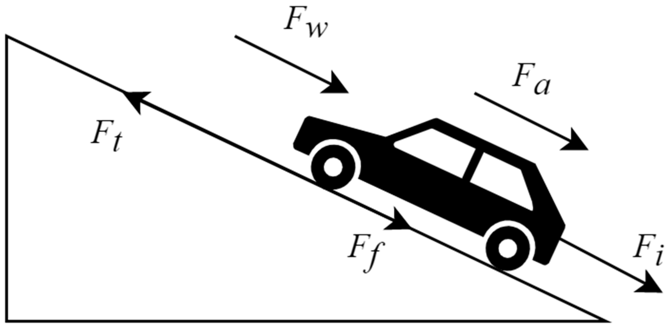
As shown in Figure 2 above, the longitudinal dynamics equation of an electric vehicle can be expressed as:

$$F_t=F_f+F_i+F_w+F_g+F_{err}$$

(1)

where $F_t$ is the driving force. According to the characteristics of electric vehicles.

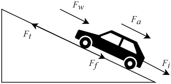
Figure 2. Diagram of electric vehicle longitudinal dynamics.

The driving force can be expressed as:

$$F_t=\frac{T_{tq}{i}_0\eta }{r}$$

(2)

where $T_{tq}$ is the motor torque, $i_0$ is the transmission ratio of the main reducer, $\eta$ is the mechanical efficiency of the transmission system, and $r$ is the rolling radius of the wheel, which is the default wheel radius when the tire pressure is sufficient.

The rolling resistance $F_f$ can be expressed as:

$$F_f=mgf\cos \alpha$$

(3)

where $m$ is the vehicle mass, $g$ is the gravitational acceleration, $f$ is the rolling resistance coefficient, and $\alpha$ is the road slope angle where the vehicle is located. It is generally considered that the road slope angle is small, $\cos \alpha \approx 1$.

The acceleration resistance $F_i$ can be expressed as:

$$F_i=\frac{\delta mdu}{dt}$$

(4)

where $\delta$ is the conversion coefficient of vehicle rotating mass, which defaults to 1 in some common algorithms. However, in actual driving conditions, $\delta$ is usually distributed between 1.1 and 1.4, and the default value of 1 will affect the accuracy of the prediction equation to a certain extent.

The air resistance $F_w$ can be expressed as:

$$F_w=\frac{C_{D}A\rho u^2}{2}$$

(5)

where $C_D$ is the air resistance coefficient, $A$ is the windward area, $\rho$ is the air density, $u$ is the vehicle speed.

The ramp resistance $F_g$, the component of gravity on the slope, can be expressed as:

$$F_g=mg sin \alpha$$

(6)

The system error $F_{err}$ is caused by uncertain environment disturbance in longitudinal dynamics [26].

To sum up, the longitudinal dynamics equation of an electric vehicle can be rewritten as [27]:

$$\frac{T_{tq}{i}_0\eta }{r}=mgf+\frac{\delta mdu}{dt}+\frac{C_{D}A\rho u^2}{2}+mgi$$

(7)

The windward area $A$ of BAIC EX360 electric vehicle used in this paper is 2.77 square meters. The air resistance coefficient $C_D$ generally takes an empirical value, and this paper sets $C_D$ as 0.3.

2.2. Prediction Equation and Observation Equation

In this paper, appropriate state variables are selected, namely, speed $u$ and road slope $i$, because they are easy to read. The state variable $x$ can be expressed as:

$$x=\left[\begin{array}{c}u\\ i\end{array}\right]$$

(8)

Generally, the slope of urban roads changes gently and the driving speed is low, so the differential equation of speed and slope can be obtained:

$$\left[\begin{array}{c}\dot{u}\\ \dot{i}\end{array}\right]=\left[\begin{array}{c}\frac{T_{tq}{i}_0\eta }{\delta mr}-\frac{fg}{\delta }-\frac{gi}{\delta }-\frac{C_{D}A\rho u^2}{2\delta m}\\ 0\end{array}\right]$$

(9)

Under urban road conditions, the vehicle speed is usually within $30\mathrm{km}/\mathrm{h}$, and the maximum is no more than $50\mathrm{km}/\mathrm{h}$. In the differential equation above, $\frac{T_{tq}{i}_0\eta }{\delta mr}$ is usually small enough to be ignored.

Based on the arithmetic relation of velocity and acceleration and the longitudinal dynamic equation of electric vehicle above, the equation of state can be set as:

$$u_k=u_{k-1}+\dot{u}\Delta t$$

(10)

$$\left[\begin{array}{c}{\dot{u}}_{k|k-1}\\ i_{k|k-1}\end{array}\right]=\left[\begin{array}{cc}1& g\Delta t\\ 0& 1\end{array}\right]\left[\begin{array}{c}{u}_{k-1}\\ i_{k-1}\end{array}\right]+\left[\begin{array}{c}\frac{\Delta t}{\delta m}\left(\frac{T_{tq}{i}_0\eta }{r}-fmg\right)\\ 0\end{array}\right]+q$$

(11)

In the above formula, ${\dot{u}}_{k|k-1}$ and $i_{k|k-1}$ represent the prior results, that is, the values at time $k$ without Kalman filtering. Additionally, $q$ is the noise vector of the prediction equation.

In the real vehicle test, the speed parameter $u_k$ can be easily measured. Therefore, this paper first takes the speed $u_k$ as the observed value and the observation equation can be expressed as:

$$Z_k=H{x}_{k|k-1}+r$$

(12)

In the observation equation, $H=\left[\begin{array}{c}1 0\\ 0 1\end{array}\right]$, indicating that both velocity and slope have been observed. Because of the immeasurable noise in the actual experiment and the substitution of empirical values in some data of the prediction equation, the error of the prediction equation cannot be ignored. Therefore, a low-precision slope observation is added in this paper. $r$ represents the measurement noise vector.

3. Adaptive Kalman Filtering

3.1. Flow Chart of Basic Kalman Filter

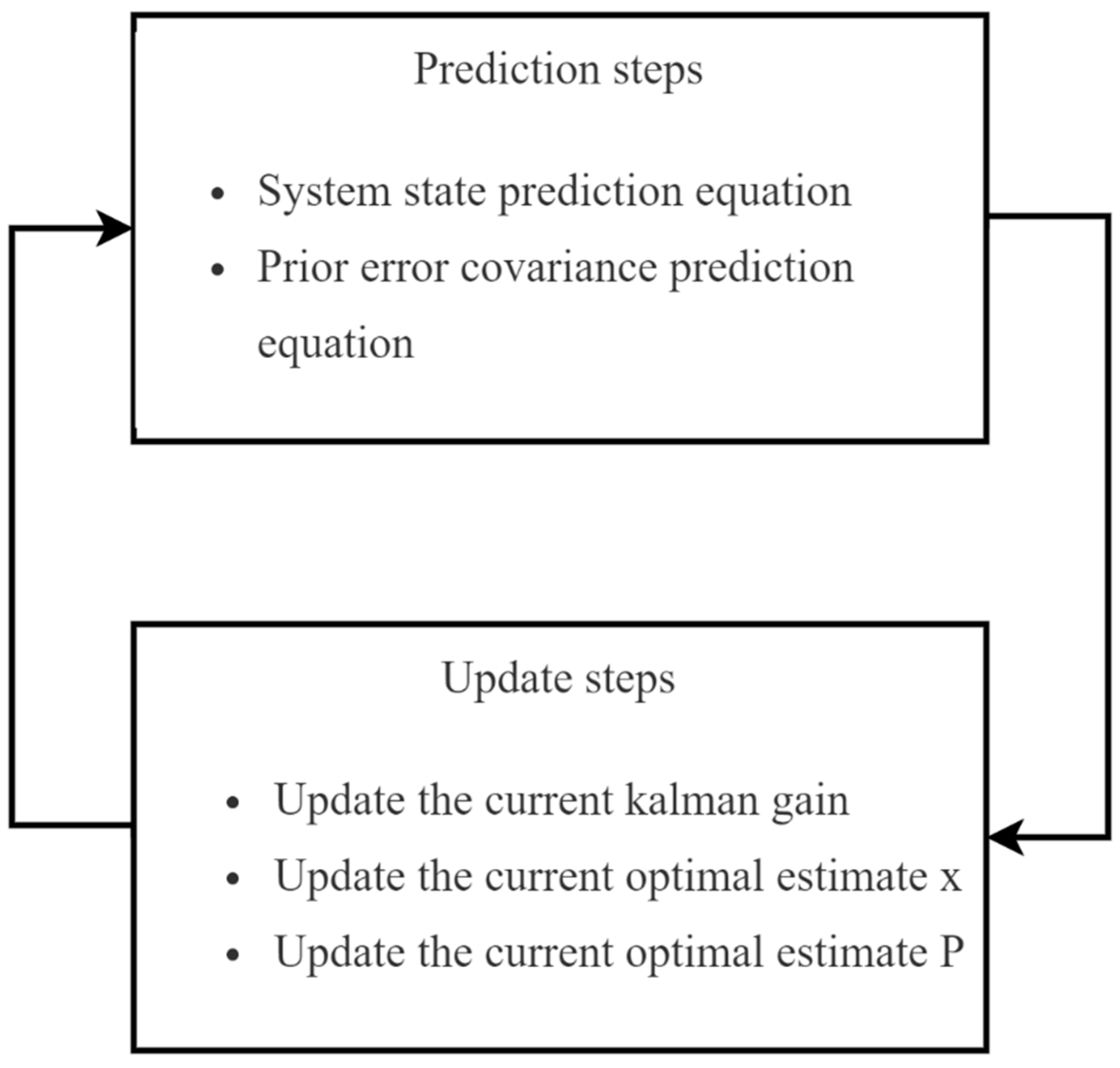
As shown in Figure 3, the application process of Kalman filter is divided into prediction and update. Kalman filter is a state optimal estimation algorithm. It calculates the priori estimate $x_{k|k-1}$ at time $k$ by substituting the optimal estimate $x_{k-1}$ at time $k-1$ into the prediction equation, compares $x_{k|k-1}$ with the measured value $Z_k$ at time $k$, assigns weights to $x_{k|k-1}$ and $Z_k$ by Kalman gain, and finally obtains the optimal estimate $x_k$ at time $k$. After that, Kalman filter recursively computes the optimal estimate at the next time.

Figure 3. Flow chart of Kalman filter.

3.2. Prediction Equations

The prediction equation of the system can be expressed as:

$$x_{k|k-1}=F{x}_{k-1}+B_{k-1}+q$$

(13)

Among them, $F=\left[\begin{array}{cc}1& g\Delta t\\ 0& 1\end{array}\right]$, $B_{k-1}=\left[\begin{array}{c}\frac{\Delta t}{\delta m}\left(\frac{T_{tq}{i}_0\eta }{r}-fmg\right)\\ 0\end{array}\right]$.

The prediction equation of the prior error covariance can be expressed as:

$$P_{k|k-1}=F{P}_{k-1}{F}^T+Q$$

(14)

where $P$ is the variance of the state estimate and represents the measure of the uncertainty in the predicted state, which comes from process error and the error of the estimate. $Q$ is the covariance matrix of prediction noise $q$.

3.3. The Update Equation

The update of Kalman gain can be expressed as:

$$K_g=P_{k|k-1}{H}^T{\left(H{P}_{k|k-1}{H}^T+R\right)}^{-}$$

(15)

where $K_g$ is Kalman gain and represents the weight relationship between predicted value and measured value. $R$ is the covariance of the observed value and represents the uncertainty of the observed state. The smaller the value is, the more accurate the observation is.

The update of the optimal estimate of $x_k$ can be expressed as:

$$x_k=x_{k|k-1}+K_g\left(Z_k-H{x}_{k|k-1}\right)$$

(16)

The update of the optimal estimate $P_k$ can be expressed as:

$$P_k=\left(I-K_{g}H\right)P_{k|k-1}$$

(17)

where $I$ represents the identity matrix, whose order is equal to the number of elements of the state variable.

3.4. Sage–Husa Adaptive Kalman Filter

Adaptive Kalman filter updates $q_k,Q_k,r_k$ and $R_k$ on the basis of Kalman filter.

A weighting coefficient $d_k$ is given, $d_k$ can be expressed as:

$$d_k=\left(1-b\right){(1-b^{k+1})}^{-}$$

(18)

where $d_k$ is usually between 0.95 and 0.99. The weighting coefficient is used to enhance the effect of recent data and update noise.

The update formula is as follows:

$$\begin{gathered} {\epsilon }_k=Z_k-H{x}_{k|k-1}-r_{k-1} \\ {q}_k=\left(1-d_k\right)q_{k-1}+d_k\left(x_k-F{x}_{k-1}\right) \\ {Q}_k=\left(1-d_k\right)Q_{k-1}+d_k\left(K_g{\epsilon }_k{\epsilon }_k^T{K}_g^T+P_k-F{x}_{k-1}{F}^T\right) \\ {r}_k=\left(1-d_k\right)r_{k-1}+d_k\left(Z_k-H{x}_{k|k-1}\right) \\ {R}_k=\left(1-d_k\right)R_{k-1}+d_k\left({\epsilon }_k{\epsilon }_k^T-H{P}_{k|k-1}{H}^T\right) \end{gathered}$$

(19)

3.5. Improved Sage–Husa Adaptive Kalman Filter

Wei et al. from Northwestern Polytechnical University studied Sage–Husa adaptive Kalman filter and found that the contribution of $Q_0$, the initial value of the covariance matrix, to $Q_k$ would decrease sharply with the increase of $k$ in the operation process, and would soon approach zero. When some systems need fixed noise with proportion, the applicability of traditional Sage–Husa adaptive Kalman filter will be reduced. The traditional Sage–Husa adaptive Kalman filter adopts the method of average information allocation for $q_k,Q_k,r_k$ and $R_k$, and the proportion of initial value to contribution is only $1/k$. At the same time, Wei et al. found in their calculation that the deviation of $q_k$ and $r_k$ would affect the coordination relationship between $R_k$ and $Q_k$, leading to the increase of subsequent deviation [15].

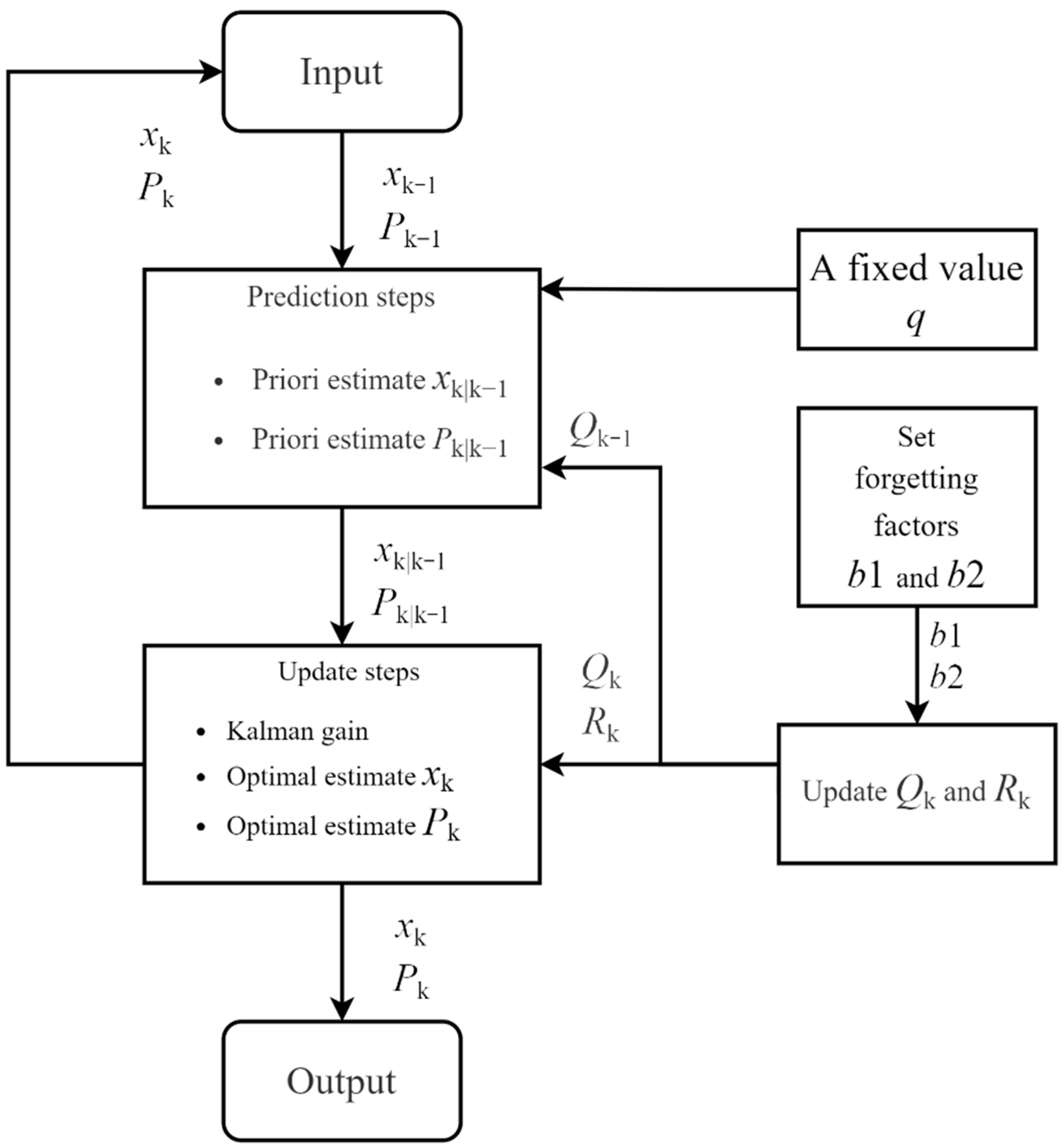
In view of the above situation, this paper improved the algorithm by canceling the calculation of $q_k$ and $r_k$, and setting the forgetting factors $b_1$ and $b_2$ respectively. The traditional Sage–Husa Kalman filter formula is rewritten as follows:

$$\begin{gathered} d_{k1}=\left(1-b_1\right){(1-b_1^{k+1})}^{-} \\ {d}_{k2}=\left(1-b_2\right){(1-b_2^{k+1})}^{-} \\ {R}_k=\left(1-d_{1k}\right)R_{k-1}+d_{1k}\left({\epsilon }_k{\epsilon }_k^T-H{P}_{k|k-1}{H}^T\right) \\ \begin{array}{c}\hfill Q_k=\left(1-d_{2k}\right)Q_{k-1}+d_{2k}(K_g{\epsilon }_k{\epsilon }_k^T{K}_g^T+P_k-F{x}_{k-1}{F}^T-2K_g{R}_k{K}_g^T\\ \hfill -2K_{g}H{P}_{k|k-1}{H}^T{K}_g^T+P_{k|k-1}{H}^T{K}_g^T+K_{g}H{P}_{k|k-1})\end{array} \end{gathered}$$

(20)

Combined with the above and Figure 4, it can be concluded that, compared with the previous algorithm, the calculation of $q_k$ and $r_k$ is cancelled, and the original forgetting factor $b$ is replaced. Instead, two forgetting factors $b_1$ and $b_2$ are set for the update of $R_k$ and $Q_k$ respectively. Meanwhile the system noise $Q_k$ is rederived by a series of approximate processing in the steps.

Figure 4. Flow chart of improved adaptive Kalman filter.

4. Experiment

4.1. Experiment Plan

In order to verify the effectiveness of the improved Sage–Husa adaptive Kalman filter for road slope estimation, a large number of vehicle tests were carried out. The driving data of multiple groups of roads with different slopes in and around southwest Forestry University in Kunming city, Yunnan Province were collected in the experiment, and the most representative groups of data were selected to verify the scheme.

4.2. Experiment Equipment and Parameters

The equipment used in the test includes BAIC New Energy EX-360 electric vehicle, on-board OBD, SD card, low-cost gyroscope, high-precision IMU and GPS. InVIEW is used as data processing and analysis software. Matlab is used to build algorithms model and produce results by inputting test data into the algorithm model.

Among them, the low-precision gyroscope is used to assist the algorithm proposed in this paper, that is, to provide rough observation value for the subsequent system to input the observation value into the algorithm. The high-precision IMU and GPS are used to provide an experimental slope value with a very small error, which can be used as a reference value for the real slope. The IMU used in this experiment is shown in Figure 5.

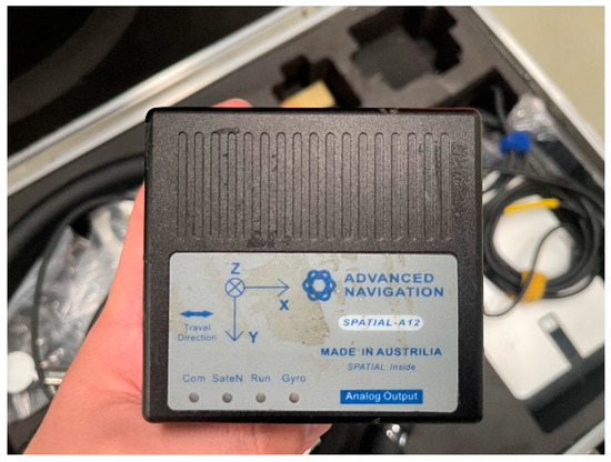
Figure 5. IMU of high accuracy.

Some vehicle parameters and model parameters are shown in Table 1 and Table 2.

Table 1. Test vehicle parameters.

Parameter	VALUE
Vehicle type	BAIC EX360
Maximum motor power	80 kW
Maximum motor torque	230 N·m
Transmission type	fixed gear ratio
Curb weight	1480 kg
Size	4110 mm × 1750 mm × 1543 mm
Transmission efficiency	97%
Tire type	205/50 R16

Table 2. Prediction model parameters.

Parameter	VALUE
r	0.3 m
m	1715 kg
δ	1.1

The tire rolling radius $r$ is the approximate tire rolling radius based on tire specification 205/50 R16 and taking into account the bearing time and sufficient tire pressure. Actual curb weight $m$ includes the quality of the car itself, the instruments and the testers. The rotational mass conversion coefficient $\delta$ of the test vehicle is derived from the empirical value of the rotational mass of the car.

4.3. Experiment Section

According to the slope classification of geomorphic detail map application of geomorphic survey and Geomorphic Mapping Commission of international Geographical Union, the slope grade is defined as 0°~0.5° plain, 0.5°~2° micro slope, 2°~5° gentle slope and 5°~15° slope. In this paper, the angle value is converted into slope value, and the data of the three groups of sections in the test are classified according to the division basis, which are micro-slope model, gentle slope model R1 and gentle slope model R2. These sections are shown in Figure 6 below.

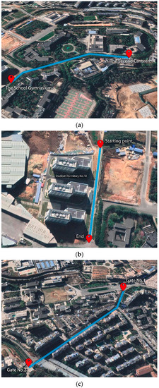
Figure 6. GPS images of the test sections. (a) Micro slope model, (b) Gentle slope model R1, (c) Gentle slope model R2.

Micro slope model: the road with a low slope, with a slope of 1 to 5%. The starting point of the road section is at the gate of the Second canteen of Southwest Forestry University, and it moves forward to the school gymnasium, then runs along the slope to the Engineering Building, and stops in the middle of the slope. The slope of this section is mostly in the range of micro-slope, so this paper regards it as a micro-slope model.

Gentle slope model R1: the road with a moderate slope, with a slope of 2 to 6%, which is located on the west side of building 19 student dormitory of Southwest Forestry University. The slope of this section is mostly in the interval of gentle slope, so this paper regards it as a gentle slope model.

Gentle slope model R2: the road with a moderate slope, with a slope of 5 to 8%. This road is a long slope from gate No. 1 to gate No. 2 of Southwest Forestry University. The slope of this section is mostly in the interval of gentle slope, so this paper regards it as a gentle slope model.

4.4. Error Analysis

In order to evaluate the accuracy of this algorithm, Root Mean Square Error (RMSE) and Mean Absolute Error (MAE) are introduced. The errors of the data obtained by the common adaptive Kalman filter algorithm and the improved Sage–Husa adaptive Kalman filter algorithm are calculated with the real data respectively, and the size of the error index is analyzed.

RMSE and MAE are expressed as follows:

$$\mathrm{RMSE}=\sqrt{\mathrm{MSE}}=\sqrt{\frac{SSE}{n}}=\sqrt{\frac{1}{n}{\displaystyle \sum }_{i=1}^n{\left(y_i-{\widehat{y}}_i\right)}^2}$$

(21)

$$\mathrm{MAE}=\frac{1}{n}{\displaystyle \sum }_{i=1}^n\left|y_i-{\widehat{y}}_i\right|$$

(22)

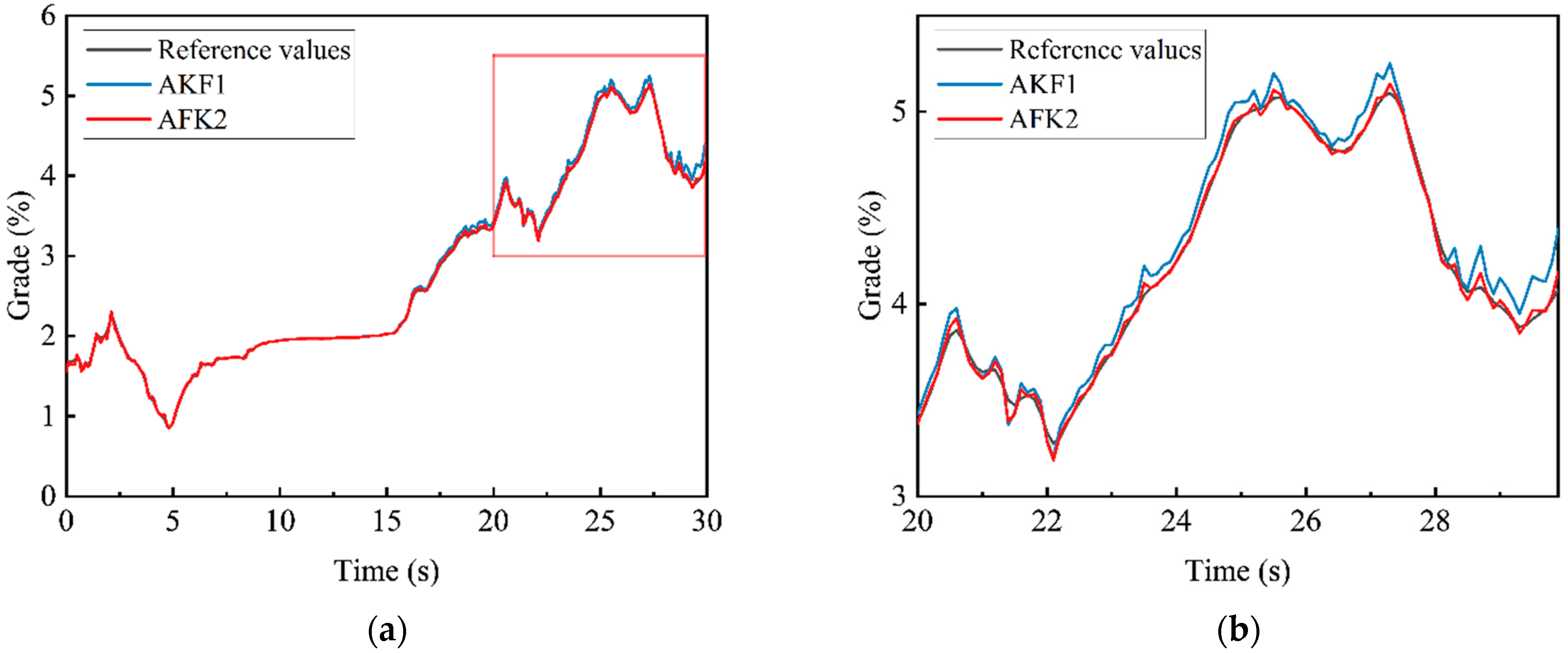
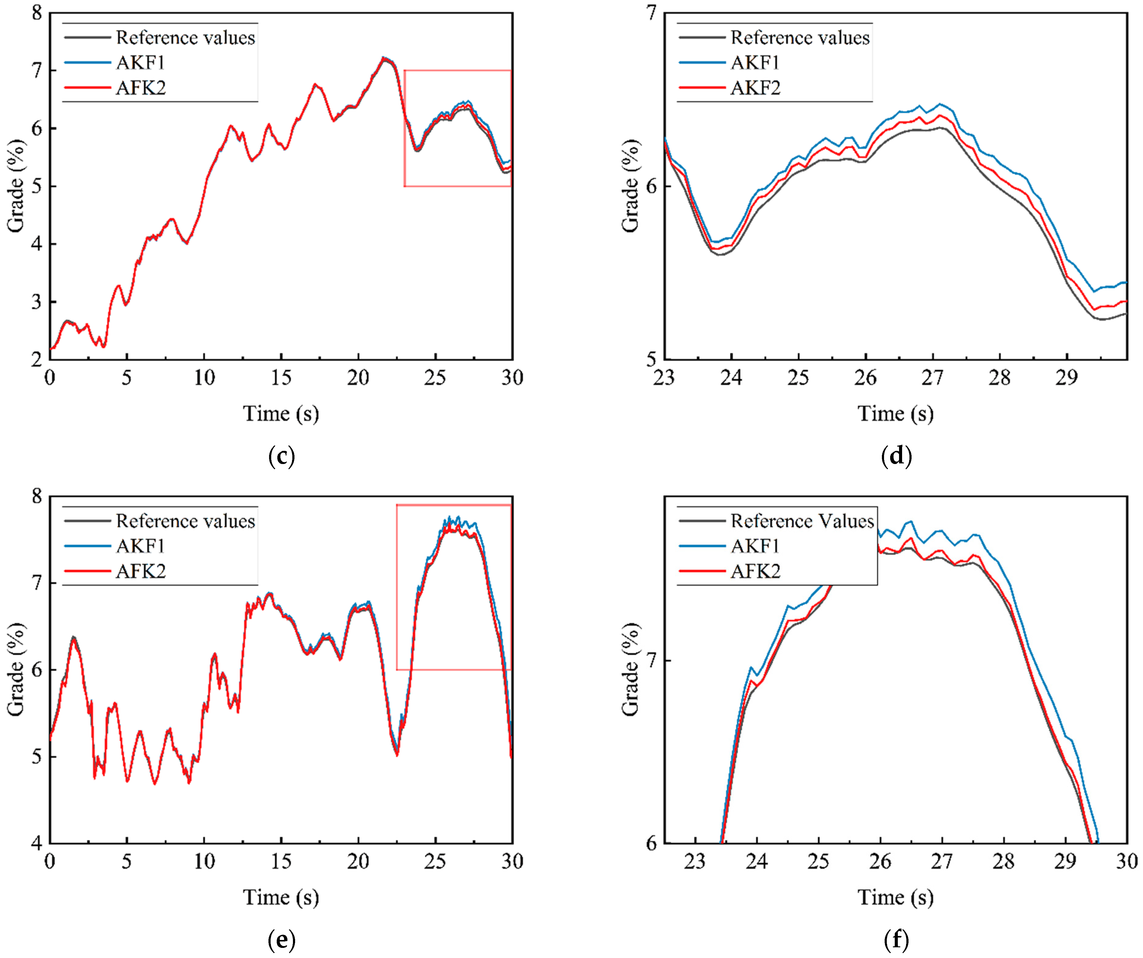
In this paper, AKF1 represents the initial adaptive Kalman filter algorithm, and AKF2 represents the improved adaptive Kalman filter algorithm. The black solid line is used to represent the reference measured road slope value, the blue solid line is used to draw the data results of the original adaptive Kalman filter algorithm, and the red solid line is used to draw the data results of the improved adaptive Kalman filter algorithm. In order to compare the two algorithms more clearly, some regions in the Figure 7 are enlarged and displayed on the right side of the original line chart. The RMSE and MAE of the algorithm results are drawn into tables, as shown in Figure 8.

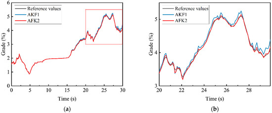
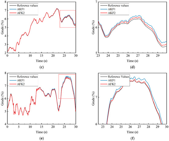
Figure 7. Contrast diagram of test effect. (a) Micro slope model, (b) part of micro slope model, (c) gentle slope model R1, (d) part of gentle slope model R1, (e) gentle slope model R2, (f) part of gentle slope model R2.

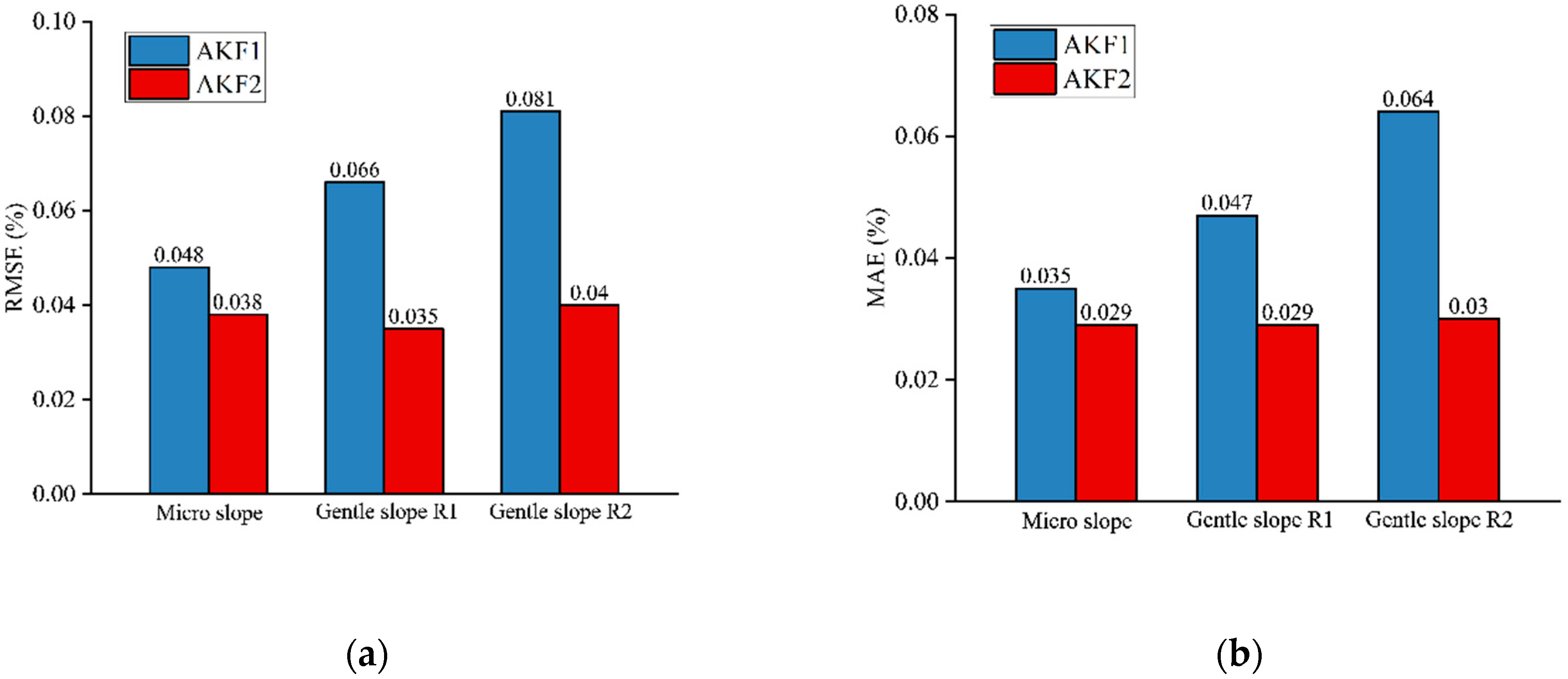
Figure 8. Comparison diagram of RMSE and MAE for two algorithms. (a) Comparison diagram of RMSE, (b) comparison diagram of MAE.

As can be seen from Figure 7 and Figure 8, the convergence speed of the two algorithms is fast. By longitudinal comparison of the two slope estimation methods under the three models, RMSE and MAE values of the original adaptive Kalman filter slope algorithm increase significantly with the increase of slope, RMSE value increases from 0.048 to 0.081%, MAE value increases from 0.035 to 0.064%, and the changes are particularly obvious. However, the RMSE and MAE values of the improved adaptive Kalman filter slope algorithm change only from 0.038 to 0.040%, and MAE from 0.029 to 0.030%. It can be concluded that the improved adaptive Kalman filter slope algorithm can better adapt to the road conditions in various slope ranges and has strong stability.

The two algorithms in the same slope range were compared horizontally. After the algorithm ran for a period of time, the accuracy of the original adaptive Kalman filter slope algorithm began to decline significantly, and errors that could not be ignored appeared. As shown in Figure 7, in the micro-slope model, the value of the original adaptive Kalman filter slope algorithm began to float significantly above the actual measured value near the moment of 24 s. In the gentle slope model R1, the error of the algorithm is more obvious when it starts near 26 s. In the gentle slope model R2, the error of the original adaptive Kalman filter slope algorithm cannot be ignored after 25 s, completely deviating from the real value. The improved adaptive Kalman filter slope algorithm can keep the data in accordance with the actual measured values in the three slope models, and will not lose the accuracy after running for a period of time.

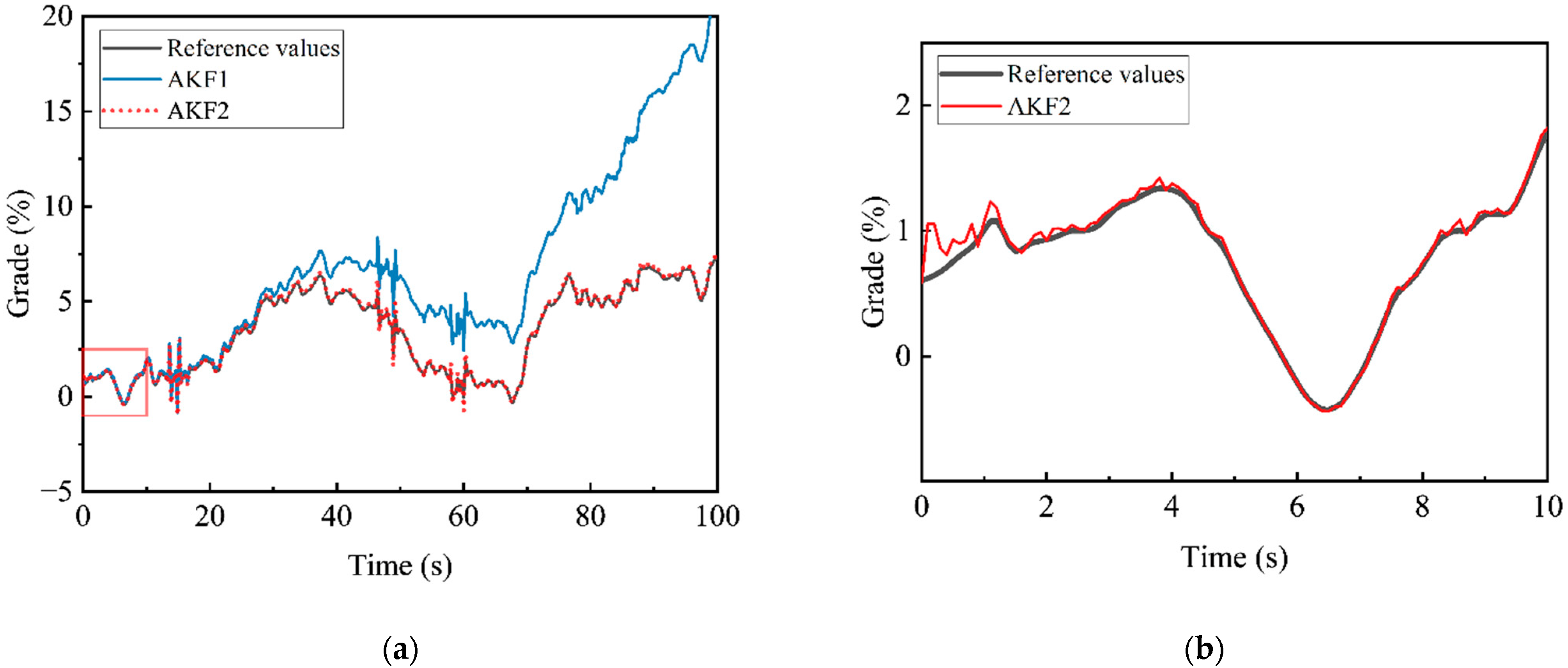
As shown in Figure 9, this paper also presents three groups of 100 s filtering results. In order to display the effect clearly, the original adaptive Kalman filter result is represented by the blue solid line, and the improved adaptive Kalman filter result is represented by the red dotted line. The filtering effect of the first few seconds is shown in the attached figure on the right. It can be seen that the error of the original adaptive Kalman filter gradually becomes obvious after a period of time. The results of the improved adaptive Kalman filter still fit the real value after a long time. From what has been discussed above, the gap between the two algorithms is greatly obvious. The RMSE value of the 100s filtering value of the slope prediction algorithm proposed in this paper increases to some extent compared with the RMSE value of the filtering value of the previous 30 s, but the result is still satisfactory.

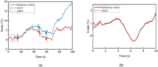
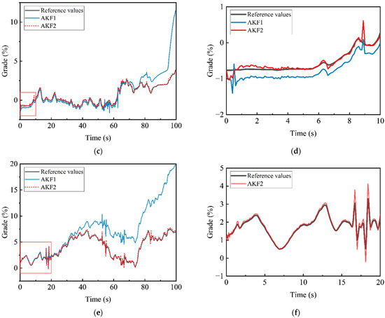
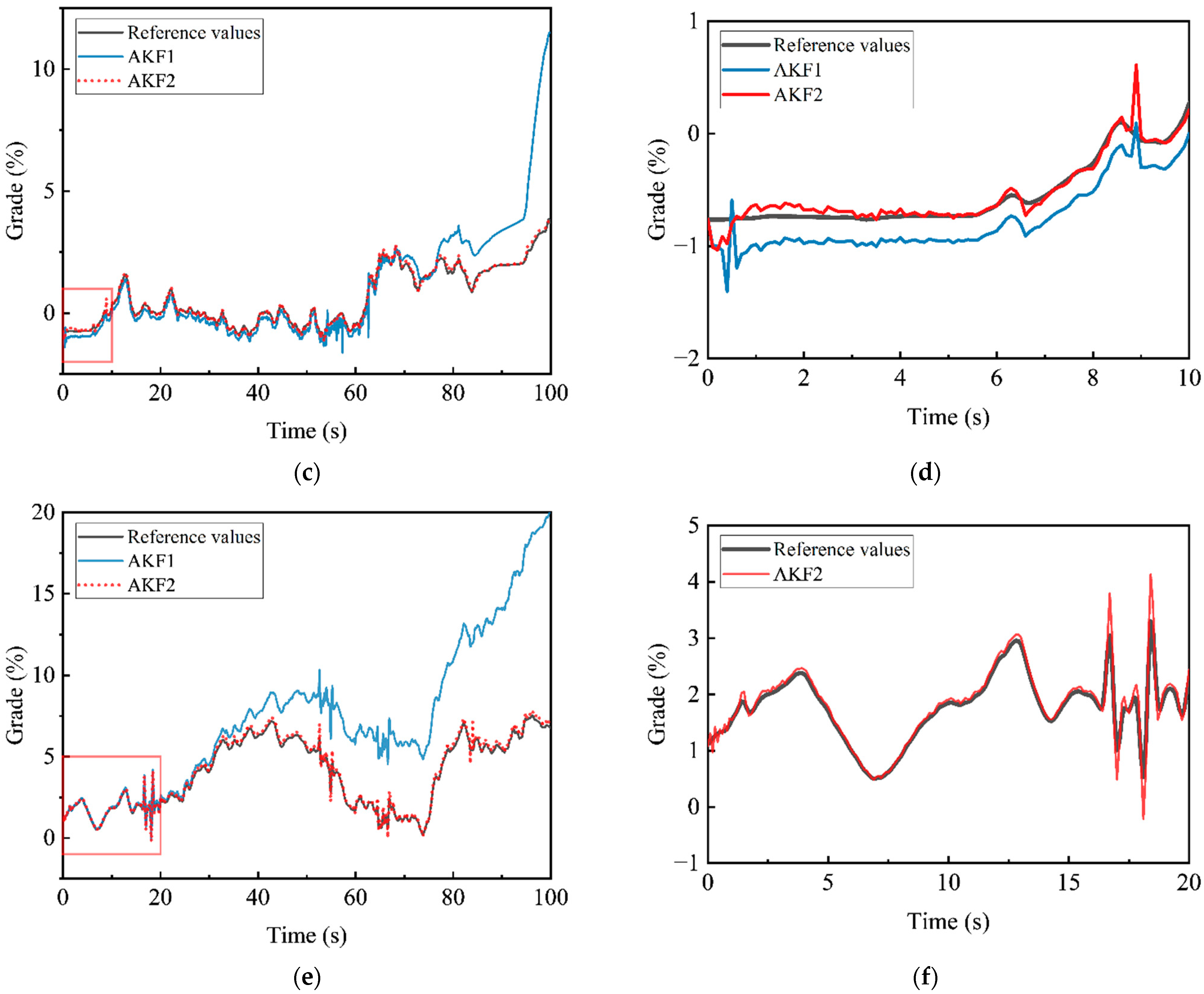
Figure 9. Contrast diagram of long-term test effect. (a) Micro slope model, (b) part of micro slope model, (c) gentle slope model R1, (d) part of gentle slope model R1, (e) gentle slope model R2, (f) part of gentle slope model R2.

Through the study and calculation of Wei et al., it is speculated that the reason for the increase of the time error may be that the recursive formula of $q_k$ and $r_k$ in the original Sage–Husa adaptive Kalman filter algorithm is the approximation of the system equation and the measurement equation. In the process of recursive accumulation, the deviation caused by the expectation of approximate mathematics may sometimes be large. However, the deviation of $q_k$ and $r_k$ will affect the coordination relationship between $Q_k$ and $R_k$, leading to the increase of subsequent deviation, thus affecting the accuracy of estimation. Taking the gentle slope model R1 as an example, the prediction equation and observation equation of the two algorithms are consistent, so the initial set values of $q_k$, $r_k, R_k$ and $Q_k$ are consistent. In the subsequent update, the two algorithms adopt different processing methods. The improved adaptive Kalman filter algorithm eliminates the calculation of $q_k$ and $r_k$, uses the variance $P$ of state estimation to approximate $Q_{k-1}$, and uses correlation substitution, so less information is discarded.

As shown in the Table 3 below, compared with the QUKF algorithm proposed by He et al., according to RMSE standards, the algorithm proposed in this paper has higher accuracy under certain conditions and uses longer scene time [1].

Table 3. Algorithm RMSE comparison.

Algorithm	AKF2			QUKF
Experiment	Test 1	Test 2	Test 3	Test 1	Test 2
RMSE	1.3%	0.8%	1.9%	7.8%	7.8%

Compared with the DUKF algorithm proposed by Jin et al., the algorithm proposed in this paper has a faster convergence speed [2]. It can be seen from Figure 9 that the convergence time of the algorithm in this paper is less than 4 s, compared with the convergence time of the DUKF algorithm of about 7 s. Within the scope of adaptive Kalman filter, the convergence speed of the algorithm proposed in this paper is faster than the AEKF algorithm proposed by Liao et al. and the AUKF algorithm proposed by Sun et al. [24,25]. In the experiment of AEKF slope estimation method proposed by Liao et al., the distance was taken as abscissa and the slope was taken as ordinate to output filtered images. It can be seen from the literature that the algorithm converges when the driving distance is about 100 m, and the convergence speed is slow. The convergence time of the AUKF algorithm proposed by Sun et al. is about 10 s, which is longer than the convergence time of the slope estimation method proposed in this paper. Therefore, this algorithm has obvious advantages in the starting stage of electric vehicles. In the starting process of pure electric vehicle, the system directly controls the motor output torque to make the vehicle start normally. When electric vehicles start, if the output torque does not adapt to the starting slope, too much output torque may lead to vehicle running forward in small slope, while too little output torque may lead to vehicle sliding behind or insufficient starting power in large slope. Therefore, the slope algorithm proposed in this paper can improve the smoothness at the start time of EV autonomous driving.

5. Conclusions

(1)

In this paper, the improved adaptive Kalman filtering algorithm draws on the valuable experience of predecessors and changes the traditional adaptive Kalman filtering algorithm. It removes the calculation of $q_k$ and $r_k$, which may lead to a sharp increase in the subsequent deviation, and reasonably improves the update of $Q_k$ and $R_k$ by using double forgetting factors $b_1$ and $b_2$.

(2)

The algorithm proposed in this paper has a wide range of application. Under the experimental data of multiple 30 s micro slope model and gentle slope model, RMSE can always be maintained within 0.04%, MAE can always be maintained within 0.03%, and short-term effect is relatively good. The RMSE and MAE can always be kept within 0.19% and 0.15%, respectively, under the demonstration of multiple groups of 100 s gentle slope model test data. Generally speaking, the algorithm is applicable to a wide range of slope and has a good general effect.

(3)

After a comprehensive comparison of the results of the two algorithms above, it can be found that, compared with the results of the original adaptive Kalman filter slope estimation method, the RMSE and MAE of the improved algorithm are significantly reduced. The RMSE of the micro slope model is reduced by 0.01%, which is 20.8% lower than the original algorithm. The MAE of the micro-slope model is reduced by 0.006%, which is 17.1% lower than the original algorithm. The RMSE of the gentle slope model R1 is reduced by 0.031%, which is 47% lower than the original algorithm. The MAE of the gentle slope model R1 is reduced by 0.018%, which is 38.3% lower than the original algorithm. The RMSE of the gentle slope model R2 is reduced by 0.041%, which is 50.6% lower than the original algorithm. The MAE of the gentle slope model R2 is reduced by 0.034%, which is 53.1% lower than the original algorithm. The error of the 100 s filtering result of the algorithm proposed in this paper increases to some extent compared with the previous 30 s filtering result. However, the error is still reasonable. In conclusion, the improved adaptive Kalman filter slope estimation method is superior.

References

- He, W.; Xi, J. A Quaternion Unscented Kalman Filter for Road Grade Estimation. In Proceedings of the 2020 IEEE Intelligent Vehicles Symposium (IV), Las Vegas, NV, USA, 19 October–13 November 2020; pp. 1635–1640. [Google Scholar]
- Jin, X.; Yang, J.; Li, Y.; Zhu, B.; Wang, J.; Yin, G. Online estimation of inertial parameter for lightweight electric vehicle using dual unscented Kalman filter approach. IET Intell. Transp. Syst. 2020, 14, 412–422. [Google Scholar] [CrossRef]
- Boada, B.L.; Boada, M.J.L.; Zhang, H. Sensor fusion based on a dual kalman filter for estimation of road irregularities and vehicle mass under static and dynamic conditions. IEEE/ASME Trans. Mechatron. 2019, 24, 1075–1086. [Google Scholar] [CrossRef] [Green Version]
- Pei, X.; Chen, Z.; Yang, B.; Chu, D. Estimation of states and parameters of multi-axle distributed electric vehicle based on dual unscented Kalman filter. Sci. Prog. 2020, 103, 0036850419880083. [Google Scholar] [CrossRef] [PubMed]
- Sun, Y.; Li, L.; Yan, B.; Yang, C.; Tang, G. A hybrid algorithm combining EKF and RLS in synchronous estimation of road grade and vehicle׳ mass for a hybrid electric bus. Mech. Syst. Signal Process. 2016, 68, 416–430. [Google Scholar] [CrossRef]
- Büyükköprü, M.; Uzunsoy, E. Reliability of Extended Kalman Filtering Technic on Vehicle Mass Estimation. J. Innov. Sci. Eng. 2021, 5, 1–11. [Google Scholar] [CrossRef]
- Li, X.; Ma, J.; Zhao, X.; Wang, L. Intelligent Two-Step Estimation Approach for Vehicle Mass and Road Grade. IEEE Access 2020, 8, 218853–218862. [Google Scholar] [CrossRef]
- Karoshi, P.; Ager, M.; Schabauer, M.; Lex, C. Robust and numerically efficient estimation of vehicle mass and road grade. In Advanced Microsystems for Automotive Applications 2017; Springer: Berlin/Heidelberg, Germany, 2018; pp. 87–100. [Google Scholar]
- Zhang, Y.; Zhang, Y.; Ai, Z.; Feng, Y.; Hu, Z. A cross iteration estimator with base vector for estimation of electric mining haul truck’s mass and road grade. IEEE Trans. Ind. Inform. 2018, 14, 4138–4148. [Google Scholar] [CrossRef]
- Jiang, S.; Wang, C.; Zhang, C.; Bai, H.; Xu, L. Adaptive estimation of road slope and vehicle mass of fuel cell vehicle. ETransportation 2019, 2, 100023. [Google Scholar] [CrossRef]
- Hu, M.; Gao, W.; Zeng, Y.; Li, H.; Yu, Z. Vehicle mass and road grade estimation based on adaptive forgetting factor RLS and EKF algorithm. In Proceedings of the 2020 5th International Conference on Power and Renewable Energy (ICPRE), Shanghai, China, 12–14 September 2020; pp. 342–346. [Google Scholar]
- Rodríguez, A.J.; Sanjurjo, E.; Pastorino, R.; Naya, M.Á. State, parameter and input observers based on multibody models and Kalman filters for vehicle dynamics. Mech. Syst. Signal Process. 2021, 155, 107544. [Google Scholar] [CrossRef]
- Bian, J.; Qiu, B.; Liu, Y.; Su, H. Adaptive Cruise Control for Electric Bus based on Model Predictive Control with Road Grade Prediction. In Proceedings of the VEHITS 2018, Funchal, Portugal, 16–18 May 2018; pp. 217–224. [Google Scholar]
- Feng, J.; Qin, D.; Liu, Y.; You, Y. Real-time estimation of road slope based on multiple models and multiple data fusion. Measurement 2021, 181, 109609. [Google Scholar] [CrossRef]
- Wei, W.; Qin, Y.Y.; Zhang, X.D.; Zhang, Y.C. Amelioration of the Sage-Husa algorithm. J. Chin. Inert. Technol. 2012, 6, 678–686. [Google Scholar] [CrossRef]
- Narasimhappa, M.; Mahindrakar, A.D.; Guizilini, V.C.; Terra, M.H.; Sabat, S.L. MEMS-based IMU drift minimization: Sage Husa adaptive robust Kalman filtering. IEEE Sens. J. 2019, 20, 250–260. [Google Scholar] [CrossRef]
- Liu, R.; Liu, F.; Liu, C.; Zhang, P. Modified sage-husa adaptive Kalman filter-based SINS/DVL integrated navigation system for AUV. J. Sens. 2021, 2021, 9992041. [Google Scholar] [CrossRef]
- Song, K.; Wang, Y.; Hu, X.; Cao, J. Online Prediction of Vehicular Fuel Cell Residual Lifetime Based on Adaptive Extended Kalman Filter. Energies 2020, 13, 6244. [Google Scholar] [CrossRef]
- Yan, W.; Ding, Q.; Chen, J.; Liu, Y.; Cheng, S.S. Needle Tip Tracking in 2D Ultrasound Based on Improved Compressive Tracking and Adaptive Kalman Filter. IEEE Robot. Autom. Lett. 2021, 6, 3224–3231. [Google Scholar] [CrossRef]
- Huang, X.; Chen, G.; Liu, Z. Sage Husa Adaptive Integrated Navigation Algorithm Based on Variable Fading Factor. In Proceedings of the 2020 International Conference on Computer Network, Electronic and Automation (ICCNEA), Xi’an, China, 25–27 September 2020; pp. 378–383. [Google Scholar]
- Zhang, F.; Yin, L.; Kang, J. Enhancing Stability and Robustness of State-of-Charge Estimation for Lithium-Ion Batteries by Using Improved Adaptive Kalman Filter Algorithms. Energies 2021, 14, 6284. [Google Scholar] [CrossRef]
- Luo, Z.; Fu, Z.; Xu, Q. An Adaptive Multi-Dimensional Vehicle Driving State Observer Based on Modified Sage–Husa UKF Algorithm. Sensors 2020, 20, 6889. [Google Scholar] [CrossRef]
- Xu, S.; Zhou, H.; Wang, J.; He, Z.; Wang, D. SINS/CNS/GNSS integrated navigation based on an improved federated Sage–Husa adaptive filter. Sensors 2019, 19, 3812. [Google Scholar] [CrossRef] [Green Version]
- Liao, X.; Huang, Q.; Sun, D.; Liu, W.; Han, W. Real-time road slope estimation based on adaptive extended Kalman filter algorithm with in-vehicle data. In Proceedings of the 2017 29th Chinese Control and Decision Conference (CCDC), Chongqing, China, 28–30 May 2017; pp. 6889–6894. [Google Scholar]
- Sun, E.; Yin, Y.; Xin, Z.; Li, S.; He, J.; Kong, Z.; Liu, X. Adaptive joint estimates of vehicle mass and road grades for small acceleration driving scenarios. J. Tsinghua Univ. Sci. Technol. 2022, 62, 125–132. [Google Scholar]
- Lin, N.; Zong, C.; Shi, S. The method of mass estimation considering system error in vehicle longitudinal dynamics. Energies 2018, 12, 52. [Google Scholar] [CrossRef] [Green Version]
- Wei, H.; He, C.; Li, J.; Zhao, L. Online estimation of driving range for battery electric vehicles based on SOC-segmented actual driving cycle. J. Energy Storage 2022, 49, 104091. [Google Scholar] [CrossRef]
Publisher’s Note: MDPI stays neutral with regard to jurisdictional claims in published maps and institutional affiliations. |
© 2022 by the authors. Licensee MDPI, Basel, Switzerland. This article is an open access article distributed under the terms and conditions of the Creative Commons Attribution (CC BY) license (https://creativecommons.org/licenses/by/4.0/).