Article

Estimation Accuracy of the Electric Field in Cable Insulation Based on Space Charge Measurement

1
Grid Innovation Res. Lab., Central Research Institute of Electric Power Industry, Yokosuka 240-0196, Japan
2
Dept. Electrical & Electronic Information Engineering, Toyohashi University of Technology, Toyohashi 441-8580, Japan
*
Author to whom correspondence should be addressed.
Energies 2022, 15(13), 4920; https://doi.org/10.3390/en15134920
Submission received: 7 June 2022 / Revised: 23 June 2022 / Accepted: 4 July 2022 / Published: 5 July 2022
(This article belongs to the Section F: Electrical Engineering)

Abstract

:
Space charge measurement accuracy is crucial when assessing the suitability of cables for high-voltage direct current (DC) systems. This study assembled state-of-the-art analysis technologies, including time-domain deconvolution, to mark electric field estimation accuracy, which the present techniques achieve. The pulse electroacoustic method was applied to a 66 kV-class extruded cable, and waveforms were obtained and analyzed to reproduce the electric field distribution. The DC voltage was set to be sufficiently low so that the analysis results can be compared with Laplace’s equation. The statistical analysis of 81 waveforms under a DC voltage of 30 kV showed that the estimation accuracy was −0.3% ± 19.9% with a 95.4% confidence interval, even with the deconvolution parameter optimized. The estimated accuracy using the “reference” waveform is applied to waveforms at higher voltages since similar estimation accuracies were confirmed for waveforms obtained under a DC voltage of 45 kV.

1. Introduction

Space charge accumulation and the resultant distortion of an electric field in cable-insulating walls are critical issues in polyethylene cables when used in high-voltage direct current (DC) transmission systems [1,2,3]. Although the space charge measurement has not been required in the test procedures for DC cables so far [4], its importance has been emphasized [5,6,7]. Along with the development of insulating materials for the high-voltage DC usage [8,9,10,11], space charge measurements have been applied to 500 kV-class cables with a 23 mm insulation thickness [12,13]. However, technological issues continue to make the data analysis difficult. The electric field distribution estimated by the space charge waveforms is sometimes unstable. This is because the impulse response (IR) of the observation system convolutes the observed waveform to distort its shape. Thus, deconvolution processing is applied to resolve the distortion. However, the convolution is expressed by the Fredholm integral equation of the first kind, and the analysis deals with ill-posed problems. Therefore, numerical low-frequency oscillations are frequently provided for distributions in the charge and electric field; an example is shown below. These numerical components in the waveform become unstable when the pulse signal width is much shorter than the insulation wall area. Such situations occur when the space charge measurement is applied to full-sized cables [14] since the pulse generator used has a short pulse width to fit its development process.
The analysis began by optimizing the deconvolution parameter so that one waveform can accurately reproduce the electric field distribution [15]. However, this process does not guarantee the accuracy of the analysis in other waveforms due to the abovementioned analysis instability. The analysis error range must be evaluated; however, little attention has been paid to the accuracy of space charge data analysis. This study employed a statistical method for evaluating the direction of the analysis results under a renowned experimental condition. The importance of the uncertainty estimation is highlighted for space charge waveforms observed for power cables. Such waveforms provide several insights, such as the field enhancement in long-term operation, and the knowledge acquired can be reflected in cable insulation design. This study proposed a method for evaluating the accuracy of space charge data analysis.
Several data processing techniques have been developed for analyzing space charge waveforms. Among the data processing techniques, the deconvolution technique has been recently updated to mitigate the aforementioned low-frequency oscillations by performing the data processing in the time domain [16], which has been developed in chemical and audio engineering [17,18,19]. Although time-domain deconvolution of space charge data has been reported [20,21,22,23], its robustness has only recently been acknowledged. Additionally, physical signal damping of space charge waveforms has also been investigated. Examples include diffusion due to the cable’s cross-sectional geometry, attenuation during the signal propagation through the insulation wall, and the effect of temperature gradients [24,25,26,27,28]. This study assembled such evaluation metrics to mark the estimation accuracy of the current technology. The accuracy evaluation reveals the key factors that arise from the analysis error range and is expected to show a direction for the analysis to become more sophisticated.
This study only deals with a simple situation where charges are induced only in inner and outer semiconductor screens and no space charges are accumulated. To detect such simple data, low DC voltage was applied and no temperature gradient was applied to a 66 kV-class extruded cable. This study concluded that the so-called “reference” waveforms were suitable for accuracy estimation. The proposed method does not require any additional measurements because such waveforms are acquired in a regular test scheme.
All measurements were carried out for the situation where charges were induced only at the electrode/insulation interfaces. However, the procedures are the same even for situations where charge accumulation occurs because analytical procedures cannot discriminate the charge origin. It follows that the analysis accuracy evaluated in this study is expected to be adopted for such latter situations. For this reason, the experimental scheme described below is referred to as the “space charge measurement”.

2. Methodology for Accuracy Evaluation

2.1. Basic Concept

Figure 1 shows the method for obtaining space charge waveforms from a regular measurement scheme to evaluate the analysis accuracy. The observation of space charge waveforms is performed under the two voltage conditions, VL and VH, and the system’s IR is extracted from the waveforms obtained under the VL condition. The basic concept of the accuracy evaluation is as follows:
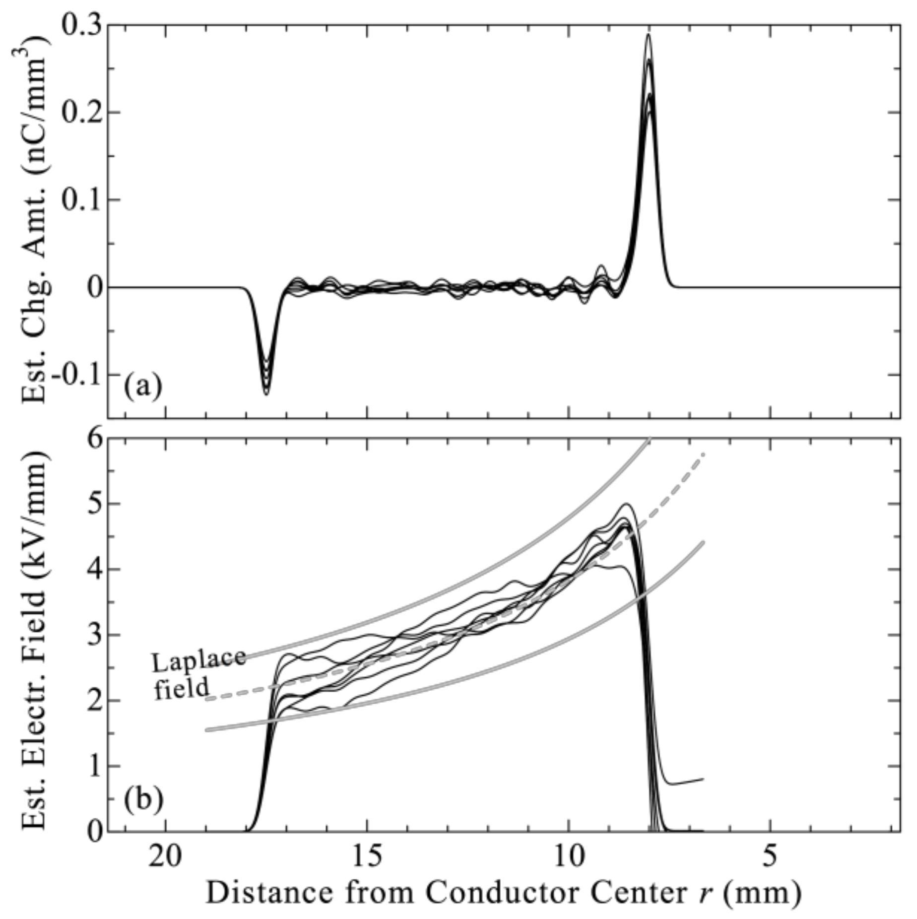
  • The accuracy evaluation is performed for field distributions estimated from waveform analyses. The field calculated for a coaxial cable using the Laplace equation is considered a reference for comparison.
  • The aforementioned accuracy evaluation provides the maximum error range of the analysis because higher DC voltages provide improved signal-to-noise ratios in the waveform.
  • The optimum IR of the system can be observed in the waveforms obtained under the VL condition. This provides an optimum analysis close to the Laplace field for waveforms observed under both VL and VH conditions.

2.2. Evaluation Flowchart

Figure 2 shows the computational flowchart for evaluating the estimation accuracy. The flowchart is categorized into three stages, from optimizing the deconvolution parameters to evaluating the estimation accuracy by analyzing waveforms obtained under the VL and VH conditions. The main flowchart begins with the selection of a waveform, v, obtained under the VL condition. The waveform v is in the form of a train of nanosecond pulses detected along the radial direction of the cable insulation wall. In the first flowchart stage, the pulse observed near the detector is regarded as an IR, which is extracted using a Tukey window. This stage performs the following time-domain deconvolution based on Tikhonov’s regularization [29]:
v′ = (tHH + λI)−1Hv
where H is the system response matrix obtained by shifting IR with an appropriate time interval, λ is the regularization parameter, I is the identity matrix, and t is the transposing operator. To optimize λ, loop computation was introduced by minimizing the assessment function in the L-curve method [30]. The deconvolution result, v′, is convoluted using a Gaussian-shaped pulse to obtain Gv′, and its norm is used for the assessment. To obtain the optimum tail position of the IR, the loop computation is doubled.
Further Gv′ correction is required as the ultrasonic waves generated within the insulation wall are partly attenuated by geometrical diffusion due to the cable curvature, and partly by dissipation when traveling through an insulator. The frequency spectra of charge pulses induced at the outer and inner screens are compared. The recovery function, f, for conducting data correction is the reciprocal of the comparison result. This process is consistent with a previous report [25].
In the second flowchart stage, the analysis accuracy is evaluated by applying the optimized deconvolution function (tHH + λI)−1H to several waveforms, v, observed under the VL condition. The deconvoluted results are integrated into the radial direction to compare with the Laplace field. Two parameters are introduced for evaluation: one is the coefficient of determination (R2), and the other is the error rate, which is the ratio of the estimated electric field to the Laplace field along with the insulation thickness. The electric field is estimated by integrating kf(Gv′), where k is the quantity needed to transform the piezoelectric outputs to the charge amount. The k-value is determined so that the double integration of kf(Gv′) matches the applied voltage at the inner screen position. In the last flowchart stage, which conforms to the second item of the basic concept, the evaluation result obtained in the second stage is verified as to whether it can be adapted to the v observed under the VH conditions.
The aforementioned evaluations are repeated by changing the IR of the system. This operation is represented by the first loop in the flowchart and conforms to the third basic concept.

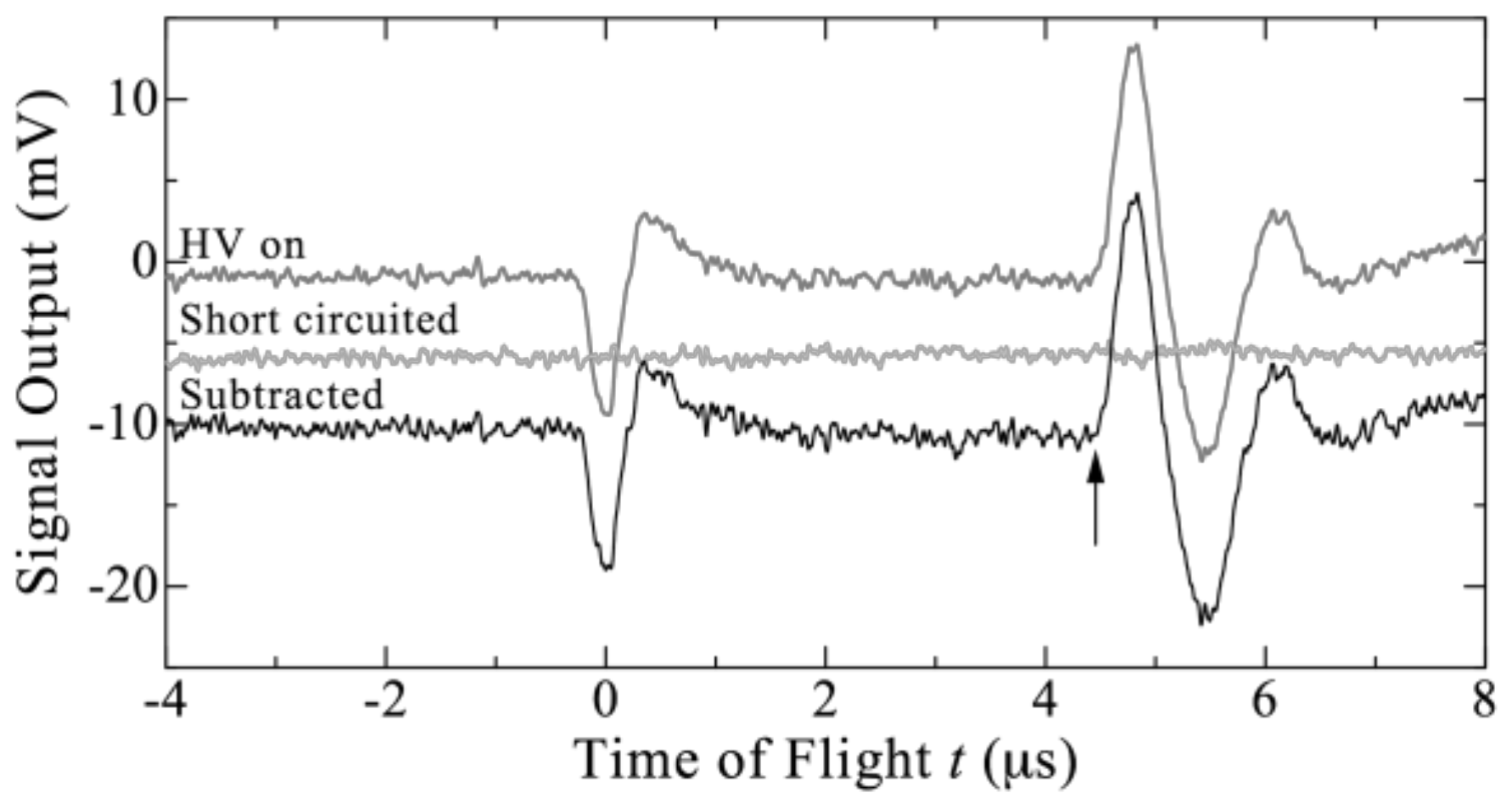
3. Experimental Procedure

The cable used for the space charge measurement was a polyethylene-insulated extruded cable manufactured for a rated alternating current voltage of 66 kV. The cross-sectional area of the cable’s conductor was 150 mm2. The inner and outer diameters of the insulation were 16 and 34 mm, respectively. The length of the cable was approximately 1.5 m. Figure 3 shows the schematic of the setup following the pulsed electroacoustic method [31,32] adopted for the cable structure [33,34]. Parts of the cable jacket and outer conductor were removed from the measurement point to attach an acoustic coupler to the outer screen and to apply square pulses. The rest of the cable serves as a coupling capacitor through the inner conductor to apply most of the pulse voltage to the measuring point [34]. Charges induced by applying the DC voltage receive a Coulombic force to generate ultrasonic waves, and their train is detected using a piezoelectric device. A DC voltage of VL = 30 kV is applied to the inner conductor so that the maximum electric field matches with the experimental condition for ‘reference measurement’ described in [15]. Another voltage VH was set to be 45 kV. A coaxial cable-based Wagner-type pulse generator [35] was handcrafted to apply square pulses with a 110 ns width and 1.5 kV voltage to the measurement point under a 50 Hz frequency. Both leading and trailing edge times of the pulse were approximately 20 ns. The limited cable length serves as the lumped capacitance, and the reflection of the pulse at the cable end can be ignored. Under both the VL and VH conditions, no space charge accumulations were observed. All measurements were conducted at room temperature.
The detector setup comprised a polymer coupling architecture [36] and a piezoelectric device made of polyvinylidene fluoride sheet with a 110 μm thickness. The detected signals were amplified by 60 dB (Spectrum SPA 1232) and obtained by averaging the waveforms 512 times using a digital phosphor oscilloscope (Tektronix MDO 4104–6). Under the VL, VH, and grounded conditions, nine waveforms were obtained. The VL data were subtracted from the grounded data to generate 81 v waveforms. This subtraction also canceled out any unwanted background signals [37]. A similar treatment was given to the VH data. The validation of the number of waveforms will be provided in Appendix A.

4. Results and Discussion

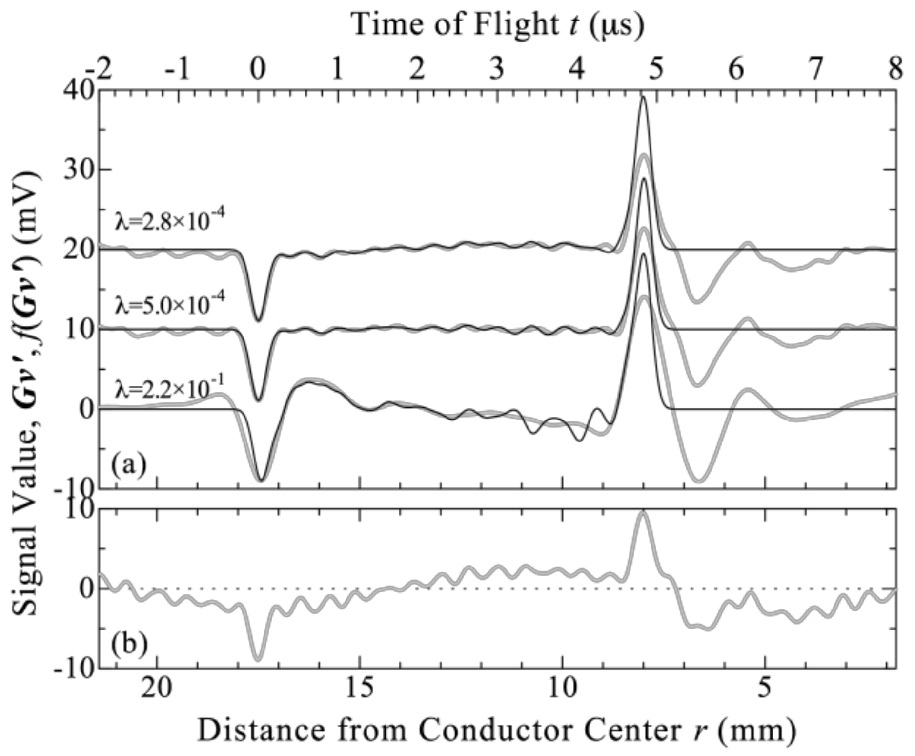
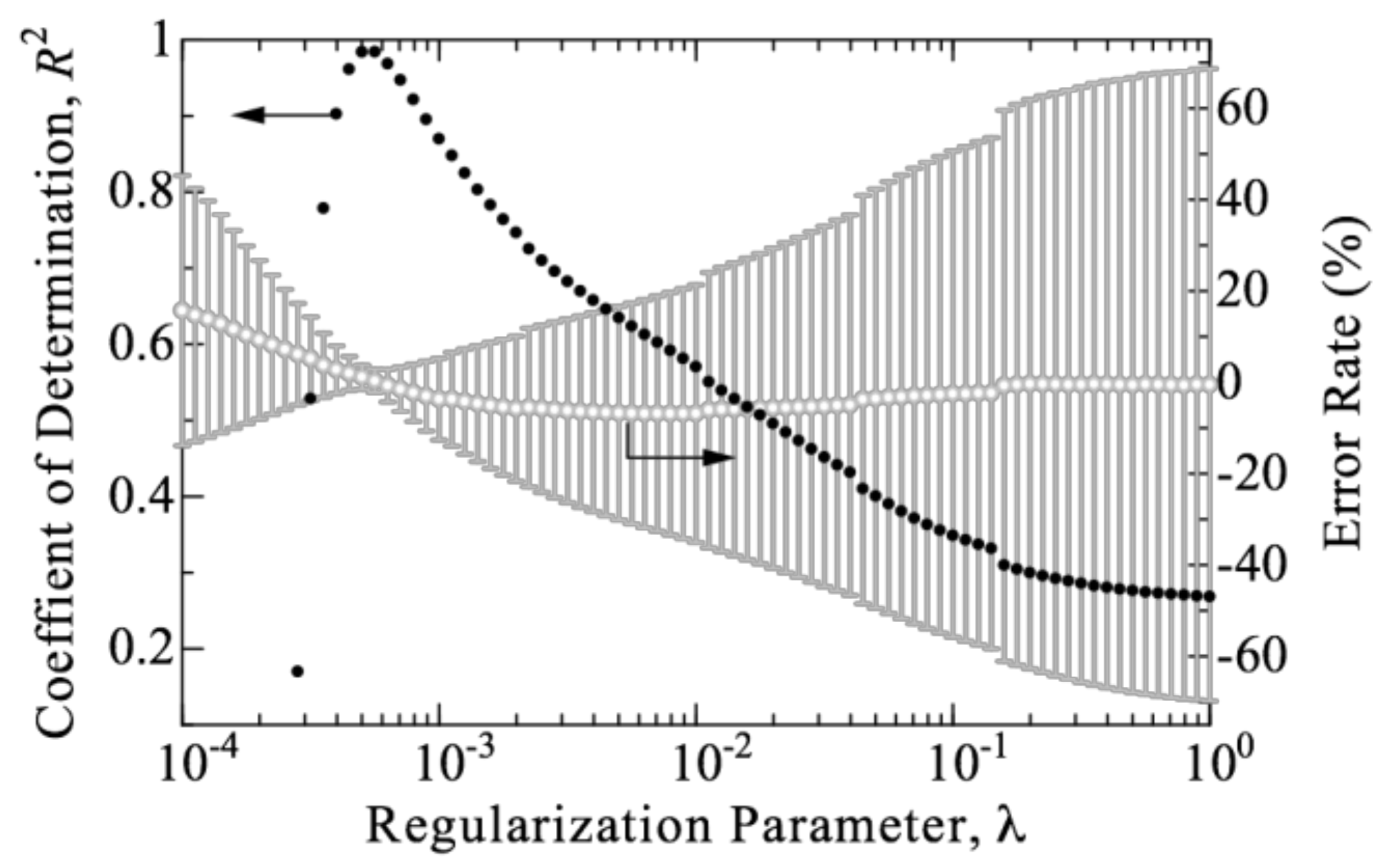
4.1. Optimization of Deconvolution Parameters (The First Stage of the Evaluation)

Figure 4 shows examples of the raw waveforms observed via measurement. Acoustic pulses were observed from the outer to inner screens, as they were detected at the time t = 0 and 4.8 μs, respectively. A latter acoustic pulse was also propagated to the detector’s opposite direction and was reflected at the conductor interface to be detected at t = 5.5 μs. This study mainly adopts such analyzer-friendly time-scale representation. Examples of the analysis results using this subtracted waveform v are shown below.
Data analysis began by extracting the pulse from the outer screen and its classification as the IR. The optimization searched for the best parameters needed to perform deconvolution against v. Figure 5 shows examples of the deconvolution results obtained by changing the regularization parameter, λ, while fixing the tail position at t = 4.39 μs. A Gaussian pulse, G, with a 220 ns full width at half maximum was used for the convolution. The low-frequency oscillation was confirmed when the deconvolution was performed in the frequency domain, whereas it was suppressed when the computation was performed in the time domain. Figure 5 also shows the attenuation correction result, f(Gv′). The analysis hereinafter excluded the reflection observed at t = 5.5 μs.
Each waveform depicted in Figure 5a was integrated along the radial direction to obtain its field and potential distribution, as shown in Figure 6. The field is enhanced near the screen when λ = 0.22, whereas it is enhanced in the bulk area when λ = 2.8 × 10⁻⁴. Such field enhancement is due to the slight heave in charge distribution, as shown in Figure 5a. The field distribution depicted in Figure 6a is consistent with the Laplace field under an R2 value of 0.30 when λ = 0.22 was used. The error rate was estimated to be 0.42% ± 63% from its average and the standard deviation along with the insulation thickness. The R2 value was 0.98, with an error rate of 1.0% ± 2.6% when λ = 5.0 × 10⁻⁴ was used. The R2 value is just an arithmetic index, but it is beneficial for optimization because it only requires the consideration of single parameters. The potential distribution experienced a minor distortion, as shown in Figure 6b, because the value at the inner screen was set to match with VL. The error rate of the field estimation was highlighted to be 16% ± 30% when the waveform obtained for the traditional frequency domain was used, although this is not shown to avoid complexity.
The L-curve method indicated that the optimum value existed around λ = 5.0 × 10⁻⁴, although this is not shown to prevent complexity. Various λ values were used to calculate the R2 and error rate of the field distribution; Figure 7 shows the results. The error rate was at its minimum for both the average and standard deviations when the R2 value was at its maximum. The optimum λ value was slightly lower than that indicated by the L-curve, similar to the case reported in [23].
The analysis was also repeated by changing the IR’s tail position. The λ value in each tail position was optimized, and the estimated field distribution was compared with the Laplace field; Figure 8 shows the result. Moreover, the best field distribution was obtained by setting the tail position to t = 4.39 μs. Under this condition, the error rate shows its minimum value for the average and standard deviation.

4.2. Accuracy Evaluation for VL Data (The Second Stage of the Evaluation)

Field distribution analysis was performed for 81 waveforms obtained under the VL condition using the optimized IR described above. Figure 9 shows some analysis examples. The estimated field is consistent with the Laplace field, with an error rate of 0.8% ± 12.0% and a 95.4% confidence interval of 0.8% ± 24.1%. These results demonstrate a certain degree of uncertainty when estimating the electric field distribution, even though the analyzed waveforms were obtained using the same method as the “reference” signal.
Such a range of error rates can be explained by error propagation. Average error rate values along the insulation thickness were recorded for each analysis result, and the histogram representation (Figure 10) showed a dispersion of 0.8% ± 6.7%. The histogram for the standard deviation of the error rate along the insulation thickness showed a deviation of 9.2%. The root-sum square of the two deviations is 11.4%, and double its value is close to the confidence interval. The results indicate that the error introduced along each electric field distribution has a significant impact on the uncertainty. The heaving remained in the field distribution, as shown in Figure 9. Its mitigation is considered the key factor in advancing the analysis.

4.3. Accuracy Evaluation for VH Data (The Third Stage of the Evaluation)

Field distribution analyses similar to those performed under the VL condition were performed for 81 waveforms obtained under the VH condition using the optimized IR described above, and the confidence interval of the estimation was 2.4% ± 22.9%, which is consistent with the result obtained in the second stage. This shows that the estimation accuracy evaluated using the “reference” waveform can be adapted to waveforms observed under higher voltage conditions.

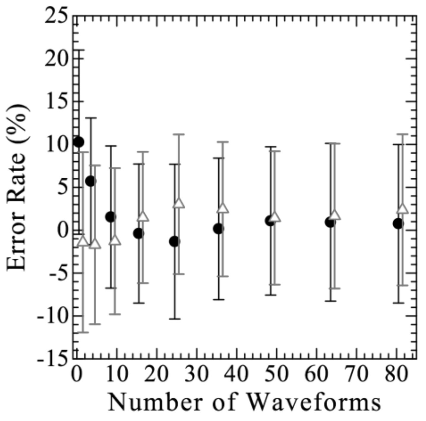
4.4. Accuracy Evaluation in Various IRs

All the aforementioned analyses were performed on the basis of the IR extracted from the waveform depicted in Figure 4. Several evaluation stages were repeated for the other 80 subtracted waveforms, and their analysis accuracies were evaluated. Figure 11 summarizes the results. The bars in Figure 11a represent the confidence interval areas. The general trend demonstrates that the accuracies estimated for the VL data are almost similar to those estimated for the VH data. This again demonstrated that the estimation accuracy can be evaluated using only the VL data. The confidence interval width narrowed as its center value approached the origin. Such a relation is reproduced in Figure 11b to increase visibility. The results indicate that the ideal IR provides both a low estimation error rate and a narrow confidence interval width. The best response obtained in this study had a confidence interval of −0.3% ± 19.9%.
The findings of this study have practical applications in cable testing. The testing voltage, VH, is selected to be high enough to possibly induce space charge accumulation in the insulation. However, the analysis of accuracy cannot be performed for such data because the field distribution itself is the subject of investigation, and the waveforms obtained are distorted. The proposed evaluation flowchart is still applied in such a situation because the accuracy evaluation can be assessed using only the VL waveform.

5. Conclusions

This study employed space charge measurement to evaluate the electric field in cable insulation, and to mark the estimation accuracy of current analysis techniques. A computational program that only requires “reference” waveforms acquired in a regular measurement scheme was constructed. Space charge waveforms were observed by applying a DC voltage, VL, of 30 kV to a 66 kV-class extruded cable. Under the viewpoint of the 95.4% confidence interval, the error range of analysis of the electric field was found to be −0.3% ± 19.9% against the estimated value, even after optimizing the deconvolution parameter. The error analysis revealed that the heaving in the estimated field distribution remained and affected the estimation accuracy.
The accuracy estimated using the “reference” waveform was effective for waveforms observed at higher voltages; thus, the accuracy estimated using the “reference” waveform is expected to be effective even when the test voltage is high enough to induce space charge accumulation and field distortion.
Future study will be conducted for situations where the temperature gradient across the insulation requires additional addressing with regards to signal attenuation. The accuracy evaluation is expected to be reflected in cable insulation design to reduce the margin against uncertainty and to contribute to the economic benefits.

Author Contributions

Conceptualization, N.F.; methodology, N.F.; software, N.F., S.M. (Shosuke Morita) and N.H.; validation, S.M. (Satoru Miyazaki); formal analysis, N.F.; investigation, N.F., S.M. (Shosuke Morita) and N.H.; resources, N.F.; data curation, N.F.; writing—original draft preparation, N.F.; writing—review and editing, T.T.; visualization, N.F.; supervision, T.T.; project administration, T.T.; funding acquisition, N.F. and T.T. All authors have read and agreed to the published version of the manuscript.

Funding

This research received no external funding.

Institutional Review Board Statement

Not applicable.

Informed Consent Statement

Not applicable.

Data Availability Statement

Not applicable.

Acknowledgments

The authors would like to express their sincere thanks to Y. Murata and T. Matsubara of Sumitomo Electric Industries for supplying the cable specimen.

Conflicts of Interest

The authors declare no conflict of interest.

Appendix A

Figure A1 shows the accuracy of the electric field distribution as a function of the number of waveforms analyzed. The IR used herein was the one optimized in Section 4.1. The field distributions described in Section 4.2 and Section 4.3 were used for the analysis. The averaged value of the error rate achieved its convergence when the number of waveforms was larger than approximately 40. The standard deviation represented by the error bar was almost consistent for the number of waveforms. The analyzed group includes 81 waveforms, which were confirmed to include all the distortions concerned.
Figure A1. Variations in the error rate of the electric field distribution, obtained by changing the number of waveforms analyzed. The circles and triangles represent the results obtained for waveforms under the VL and VH conditions, respectively. The error bar represents their standard deviation. Plots were horizontally shifted to increase visibility.
Energies 15 04920 g0a1

References

  1. U.S. Energy Information Administration. Assessing HVDC Transmission for Impacts of Non-Dispatchable Generation. Available online: https://www.eia.gov/analysis/studies/electricity/hvdctransmission/ (accessed on 31 May 2022).
  2. Fukagawa, H.; Miyauchi, H.; Yamada, Y.; Yoshida, S.; Ando, N. Insulation properties of 250 kV DC XLPE cables. IEEE Trans. Power Appar. Syst. 1981, 100, 3175–3184. [Google Scholar] [CrossRef]
  3. Ando, N.; Numajiri, N. Experimental investigation of space charge in XLPE cable using dust figure. IEEE Trans. Electr. Insul. 1979, 14, 36–43. [Google Scholar] [CrossRef]
  4. CIGRE. Recommendations for Testing DC Extruded Cable Systems for Power Transmission at a Rated Voltage up to 500 kV; CIGRE Technical Brochure 496; CIGRE: Paris, France, 2012. [Google Scholar]
  5. Mazzant, G.I.; Marzinotto, M.; Castellon, J.; Chen, G.; Fothergill, J.; Fu, M.; Hozumi, N.; Lee, J.-H.; Li, J.; Mauseth, F.; et al. IEEE Recommended Practice for Space Charge Measurements on High-Voltage Direct-Current Extruded Cables for Rated Voltages up to 550 kV; IEEE Std. 1732; IEEE Dielectrics and Electrical Insulation Society: New York, NY, USA, 2017. [Google Scholar] [CrossRef]
  6. CIGRE. Recommendations for Testing DC Extruded Cable Systems for Power Transmission at a Rated Voltage Up to and Including 800 kV; CIGRE Technical Brochure 852; CIGRE: Paris, France, 2021. [Google Scholar]
  7. Albertini, M.; Franchi Bononi, S.; Giannini, S.; Mazzanti, G.; Guerrini, N. Testing challenges in the development of innovative extruded insulation for HVDC cables. IEEE Electr. Insul. Mag. 2021, 37, 21–32. [Google Scholar] [CrossRef]
  8. Mazzanti, G.; Marzinotto, M. Extruded Cables for High-Voltage Direct-Current Transmission: Advances in Research and Development; Wiley-IEEE Press: Hoboken, NJ, USA, 2013. [Google Scholar]
  9. Du, B. (Ed.) Polymer Insulation Applied for HVDC Transmission; Springer: Singapore, 2021. [Google Scholar]
  10. Huang, X.; Tanaka, T. (Eds.) Polymer Composites for Electrical Engineering; Wiley-IEEE Press: Hoboken, NJ, USA, 2021. [Google Scholar]
  11. Thabet, A.M. Emerging Nanotechnology Applications in Electrical Engineering. IGI Global: Hershey, PA, USA, 2021. [Google Scholar]
  12. Yamanaka, T.; Maruyama, S.; Tanaka, T. The development of DC+/−500 kV XLPE cable in consideration of the space charge accumulation. In Proceedings of the 7th International Conference on Properties and Applications of Dielectric Materials, Nagoya, Japan, 1–5 June 2003; pp. 689–694. [Google Scholar] [CrossRef]
  13. Igi, T.; Mashio, S.; Sakamaki, M.; Kazama, T.; Sasaki, K.; Nishikawa, S. System performance and demonstration of 400 kV–525 kV DC-XLPE cable and accessories. In Proceedings of the International Symposium on HVDC Cable Systems, Dunkirk, France, 8–10 November 2017. [Google Scholar]
  14. Morita, S.; Fuse, N.; Takahashi, T.; Matsubara, T.; Murata, Y.; Zahra, S.; Hozumi, N. Space charge measurement of full-size 23-mm-thick XLPE cables in load cycle condition. In Proceedings of the Jicable HVDC ’21: International Symposium on HVDC Cable Systems, Liege, Belgium, 8–10 November 2021. [Google Scholar]
  15. IEC TS 62758; Calibration of Space Charge Measuring Equipment Based on the Pulsed Electro-Acoustic (PEA) Measurement Principle. International Electrotechnical Commission: Geneva, Switzerland, 2012.
  16. Hozumi, N.; Prastika, E.B.; Zahra, S.; Kawashima, T.; Murakami, Y. Dual-domain deconvolution process applied to time-resolved quantitative dielectric measurement. In Proceedings of the IEEE 3rd International Conference on Dielectrics, Virtual, 5–31 July 2020; pp. 347–350. [Google Scholar] [CrossRef]
  17. Gugliotta, L.M.; Vega, J.R.; Meira, G.R. Instrumental broadening correction in size exclusion chromatography. Comparison of several deconvolution techniques. J. Liq. Chromatogr. 1990, 13, 1671–1708. [Google Scholar] [CrossRef]
  18. Bányász, Á.; Keszei, E. Model-free deconvolution of femtosecond kinetic data. J. Phys. Chem. A 2006, 110, 6192–6207. [Google Scholar] [CrossRef] [PubMed] [Green Version]
  19. Norcross, S.G.; Soulodre, G.A.; Lavoie, M.C. Subjective investigations of inverse filtering. J. Audio Eng. Soc. 2004, 52, 1003–1028. [Google Scholar]
  20. Bloss, P.; Reggi, A.S. Application of the regularization technique to the deconvolution of thermal pulse data. In Proceedings of the 9th International Symposium on Electrets, Shanghai, China, 27 September 1996; pp. 171–176. [Google Scholar] [CrossRef]
  21. Hu, L.; Zhang, Y.; Zheng, F. Novel numerical methods for measuring distributions of space charge and electric field in solid dielectrics with deconvolution algorithm. IEEE Trans. Dielectr. Electr. Insul. 2005, 12, 809–814. [Google Scholar] [CrossRef]
  22. Vissouvanadin, B.; Vu, T.T.N.; Berquez, L.; Roy, S.; Teyssèdre, G.; Laurent, C. Deconvolution techniques for space charge recovery using pulsed electroacoustic method in coaxial geometry. IEEE Trans. Dielectr. Electr. Insul. 2014, 21, 821–828. [Google Scholar] [CrossRef]
  23. Gupta, A.; Reddy, C.C. On the estimation of actual space charge using pulsed electro-acoustic system. IEEE Trans. Dielectr. Electr. Insul. 2016, 23, 3086–3093. [Google Scholar] [CrossRef]
  24. Liu, R.; Takada, T.; Takasu, N. Pulsed electro-acoustic method for measurement of space charge distribution in power cables under both dc and ac electric fields. J. Phys. D Appl. Phys. 1993, 26, 986–993. [Google Scholar] [CrossRef]
  25. Li, Y.; Aihara, M.; Murata, K.; Tanaka, Y.; Takada, T. Space charge measurement in thick dielectric materials by pulsed electroacoustic method. Rev. Sci. Instrum. 1995, 66, 3909–3916. [Google Scholar] [CrossRef]
  26. Nagashima, K.; Tanaka, Y.; Takada, T.; Qin, X. Effect of cylindrical function on measurement of space charge distribution in coaxial cable insulator using PEA method. IEEJ Trans. Power Energy 1999, 119, 853–860. [Google Scholar] [CrossRef] [Green Version]
  27. Wang, H.; Wu, K.; Zhu, Q.; Wang, X. Recovery algorithm for space charge waveform under temperature gradient in PEA method. IEEE Trans. Dielectr. Electr. Insul. 2015, 22, 1213–1219. [Google Scholar] [CrossRef]
  28. Morita, S.; Kawashima, T.; Murakami, Y.; Hozumi, N. Study on correction method of signal distortion under temperature gradient for space charge measurement of HVDC cables. IEEJ Trans. Power Energy 2020, 140, 271–276. [Google Scholar] [CrossRef]
  29. Tikhonov, A.N. On the stability of inverse problems. Computes Rendus (Doklady) de l’Academie des Sciences de l’URSS 1943, 39, 176–179. [Google Scholar]
  30. Hansen, P.C. Analysis of discrete ill-posed problems by means of the L-curve. Soc. Ind. Appl. Math. Rev. 1992, 34, 561–580. [Google Scholar] [CrossRef]
  31. Maeno, T.; Kushibe, H.; Takada, T. Pulsed electro-acoustic method for the measurement of volume charges in e-beam irradiated PMMA. In Proceedings of the Conference on Electrical Insulation & Dielectric Phenomena, New York, NY, USA, 20–24 October 1985; pp. 389–397. [Google Scholar] [CrossRef]
  32. Li, Y.; Takada, T. Progress in space charge measurement of solid insulating materials in Japan. IEEE Electr. Insul. Mag. 1994, 10, 16–28. [Google Scholar] [CrossRef]
  33. Fukunaga, K.; Miyata, H.; Sugimori, M.; Takada, T. Measurement of charge distribution in the insulation of cables using pulsed electroacoustic method. IEEJ Trans. Fundam. Mater. 1990, 110, 647–648. [Google Scholar] [CrossRef] [Green Version]
  34. Hozumi, N.; Okamoto, T.; Imajo, T. Space charge distribution measurement in a long size XLPE cable using the pulsed electroacoustic method. In Proceedings of the Conference Record of the 1992 IEEE International Symposium on Electrical Insulation, Baltimore, MD, USA, 7–10 June 1992; pp. 294–297. [Google Scholar] [CrossRef]
  35. CIGRE. Guide for Space Charge Measurements in Dielectrics and Insulating Materials; CIGRE Technical Brochure 288; CIGRE: Paris, France, 2006. [Google Scholar]
  36. Zahra, S.; Morita, S.; Utagawa, M.; Kawashima, T.; Murakami, Y.; Hozumi, N.; Morshuis, P.; Cho, Y.; Kim, Y. Space charge measurement equipment for full-scale HVDC cables using electrically insulating polymeric acoustic coupler. IEEE Trans. Dielectr. Electr. Insul. 2022, 29, 1053–1061. [Google Scholar] [CrossRef]
  37. Chen, G.; Chong, Y.L.; Fu, M. Calibration of the pulsed electroacoustic technique in the presence of trapped charge. Meas. Sci. Technol. 2006, 17, 1974–1980. [Google Scholar] [CrossRef] [Green Version]
Figure 1. Schematic of the measurement schedule. Waveforms obtained under short-circuited and voltage-applied conditions are subtracted to create the data to be analyzed.
Energies 15 04920 g001
Figure 2. Flowchart for evaluating the analysis accuracy.
Energies 15 04920 g002
Figure 3. Cross-section schematic of the space charge measurement for a cable based on the pulsed electroacoustic method.
Energies 15 04920 g003
Figure 4. Acoustic waveform examples for voltage-on and -off conditions. The waveforms were vertically shifted to increase visibility. The arrow represents the tail position of the IR used for analysis in Figure 5, Figure 6 and Figure 7.
Energies 15 04920 g004
Figure 5. Results of the deconvolution performed on time domain (a) and frequency domain (b) obtained for the subtracted waveform shown in Figure 4, where the tail of the IR is shown by an arrow. The deconvoluted pulse was replaced by the Gaussian shape to be represented as Gv′ with gray curves. Attenuation correction was superimposed to be represented as f(Gv′) with black curves. The waveforms in (a) were vertically shifted, and the horizontal line was inserted in (b) to increase visibility.
Energies 15 04920 g005
Figure 6. Estimated electric field (a) and potential (b) obtained by integrating the charge distribution shown in Figure 5a. The gray curve in (a) shows the field distribution calculated from Laplace’s equation. This curve was extrapolated to the inner and outer semiconductive layer areas to increase visibility.
Energies 15 04920 g006
Figure 7. The R2 value and error rate of the estimated field distribution against the Laplace field obtained by changing the regularization parameter, λ, for the IR used in Figure 5 and Figure 6. The error bar represents the standard deviation of the error rate along the insulation thickness.
Energies 15 04920 g007
Figure 8. R2 value and error rate of the estimated field distribution obtained by IRs optimized for various tail positions. The error bar represents the standard deviation of the error rate along the insulation thickness.
Energies 15 04920 g008
Figure 9. Examples of charge (a) and electric field distribution (b) estimated for several space charge data obtained by applying the DC voltage of VL. The gray curves in (b) represent the field curve calculated from Laplace’s equation. The 95.4% confidential interval area is also shown. These curves were extrapolated to the inner and outer conductive layer areas to increase visibility.
Energies 15 04920 g009
Figure 10. Histogram of the estimation accuracy of the electric field against the Laplace field evaluated for 81 waveforms obtained under the VL condition.
Energies 15 04920 g010
Figure 11. (a) Mutual relationship between the estimation accuracies of the electric field distribution estimated for the space charge waveforms, v, obtained for VL = 30 kV and VH = 45 kV. Each plot represents the accuracy evaluation results for the different 81 IRs. The error bars represent the width of a 95.4% confidence interval. The relationship between the mean and the confidence interval of the error rate under the VL condition was reproduced in (b) to increase visibility.
Energies 15 04920 g011
Publisher’s Note: MDPI stays neutral with regard to jurisdictional claims in published maps and institutional affiliations.

