Abstract
Simulation models of transport systems are a key tool for solving many problems in the field of management of these systems. The methodologies for creating such models use datasets on both transport infrastructure and demand for the delivery of goods or passenger transport, however, many factors are considered based on assumptions due to the complexity. This article describes the approach to modeling the cargo transportation system for road transport in Poland based on data obtained by the Central Statistical Office from the TD-E survey. This approach avoids many assumptions about demand as the demand parameters are estimated based on a sample representing the general population—a set of all economic entities generating freight traffic. Basic procedures in the developed approach have been implemented as Python scripts. As a result of the use of the proposed methodology, a country-wide road transport model was obtained based on the TD-E survey from 2018. The adequacy of the developed model was assessed based on the results of the General Traffic Measurement from 2015. The obtained model is of satisfactory quality (the coefficient of determination equals 0.62), which can be improved after calibrating the space resistance functions and improving the traffic distribution procedure.
1. Introduction
Researching traffic behavior helps to resolve a lot of problems related to the transport sector: from minimizing congestion and reducing negative environmental impact, to improving efficiency and optimizing the whole transportation system. For many years the implementation of the transportation system model has remained the most powerful and fundamental instrument for conducting studies on complex real-world transport systems, their components, and the relations among those components [1,2]. The results achieved from a thorough model analysis support researchers, policymakers, and transport planners in comprehension and interpretation of real-life processes and serve as a tool to solve various problems and challenges in the field of transport.
Due to rapid technological progress, economic growth, and urbanization, one of the most significant transport problems has become a quick increase in demand for transport services, which exceeds the possibilities of its fulfillment. As the solution to this challenge, the development of more sustainable transport systems may be proposed. Such systems should be capable of satisfying existing transport demand [3], should guarantee the transition to electrification of road vehicles [4], and must provide a fundamental shift from heavy road trucks towards light vehicles [5], etc.
The current study aims to create a country-wide simulation model of the road transport system to estimate the traffic volume on sections of the road network and transportation work performed by freight vehicles.
The use of a simulation model of the road transport system powered in real-time by current statistical data allows:
- Estimating the size of the generated and absorbed heavy traffic in traffic areas without carrying out expensive questionnaire surveys;
- Forecasting the transport work generated by economic units for domestic and foreign transport;
- Estimating the load on given sections of the road network;
- Forecasting load changes and congestion of road network sections in the case of closure or short-term shutdown of selected sections of the network.
A significant limitation in this research related to developing the transport system model was the inability to use specialized computer programs (e.g., PTV Visum or Aimsum); the reason was that the purchase of commercial licenses for such software by the end user (the Central Statistical Office of Poland) was not included in the budget of the research project.
The paper has the following structure: Section 2 contains a brief review of the recent literature in the field of transport modeling and forecasting; Section 3 presents the proposed approach to modeling the road transport system of Poland for deliveries of cargoes; Section 4 depicts the software developed to implement the proposed approach; Section 5 discusses the simulation results and the adequacy of the obtained model; Section 6 contains the conclusions.
2. Literature Review
The first stage of almost every transport modeling is transport demand forecasting and choosing a method for its evaluation. A large number and wide variety of these methods (qualitative and quantitative) allow the forecaster to select the appropriate technique and most accurately analyze and predict the demand for transport services [6].
The traditional four-step travel model, due to its universality and continuous improvements, is one of the most frequently used approaches for modeling transport demand and consequently for transport planning. This complex decision-making process, transport planning, includes such tasks as transport infrastructure evaluation and implementation, exploration of policies and technologies, distribution management, and other activities aiming at the improvement or designing of new traffic scenarios [7]. In the conventional form, the four-step travel model includes the following steps: trip generation, trip distribution, modal split, and route assignment. The first step characterizes the number of produced or attracted trips in the analyzed region. Further, considering the spatial parameter, the trip is created by matching trip origins and destinations. In the third stage, the proportion of trips that use specific travel modes is evaluated and the last step assigns trips between the origin and destination by forming a route [2,8,9].
However, despite the widespread use of the four-step modeling approach, some researchers argue about the suitability of such a model for current freight transport development. For instance, the authors of [10] state that there is a need for the development of new freight transport demand predicting models that consider the transformations in the transport sector and its structure. As an alternative to the four-step model, the authors propose the application of models that examine the behavior of all the actors involved in decision-making throughout the delivery process. Additionally, the limitations of the four-step model in the perception of so-called 6D-variables (density, diversity, design, destination, distance, and demand management) are indicated in [11]. Another methodology, which aims to improve the travel demand forecasting in the trip distribution step of the model, was proposed by the authors of [12]. For such purposes, multilevel logistic regression, which incorporates extra environmental variables, was applied by the authors of the methodology. The complexity of implementation, analysis, and testing of the demand models was emphasized by the results of [13].
On the other hand, the usefulness and suitability of the four-step travel model in modern conditions are confirmed by its application in many recent scientific studies, which have obtained significant results [14]. For instance, the combination of the travel model with actual transport demand indicators was used for the development of a route-planning tool [15]. The presented solution was implemented using the transport network simulation in PTV Visum software, the Budapest Macroscopic Transport Model, and provides users with route suggestions based on dynamically changing demand parameters. Up-to-date information on actual demand is received by the system every 15 min and updates the system’s functioning. Another research project used the adjusted four-step algorithm to solve the vehicle scheduling problem, aiming to minimize the number of serving vehicles for the on-demand transport services [16]. The authors propose to incorporate on-demand services into the macroscopic travel demand model, expanding the model by adding supplementary steps to the conventional four. The model was tested on existing survey data for several operational scenarios and the output indicates the possibility of reducing the number of serving vehicles. Authors of [17] focused on demand behavior modeling for intermodal travel. For this purpose, researchers used a microscopic multi-agent traffic demand model, mobiTopp, which allows applying the intermodality to the destination and mode choice models, and further, a route choice step was implemented in PTV Visum software. The authors of [18] aim to help transportation planners and analysts in evaluation, prediction, and mobility management by developing a framework that supports measuring OD matrices. The combination of traditional data from surveys and big data (floating car data) for estimation of travel demand increased the accuracy of the traditional demand model. The authors of [19] used data from open sources and generic data in modeling commercial travel demand to analyze commercial transportation. By applying cluster analysis, a passenger transport model, and land-use model, researchers achieved an instrument that allows analyzing different scenarios of commercial transportation for dynamically changing conditions.
One of the main purposes of traffic simulation modeling is to simulate vehicle movement for further analysis, predict traffic conditions, and optimize the transport network. Nowadays, a large variety of traffic simulation models is presented in the scientific literature. Such models require detailed input traffic and infrastructure parameters regarding actual traffic conditions, which include such data as characteristics of travel demand, representation of the road network, and infrastructure. Significantly important components of traffic modeling are the sources and methods of obtaining, processing, and validating data for the simulation [20]. Among the most common sources of data are questionnaires and interviews, existing literature, statistical reports (the national household survey, traffic count and population data, datasets from a road authority, etc.), information collected in the field as well as data obtained from intelligent transport systems.
Traffic simulation models are classified into different groups depending on the input parameters, the degree of detail of the output, area of application, and other factors. Depending on the level of detail, traffic models are usually divided into macroscopic, mesoscopic, microscopic, and hybrid [21]. The macroscopic type of model represents traffic flow as an integrated/flowing stream, microscopic depicts the behavior of individual participants of the transport process on a very precise level, and mesoscopic contains the characteristics of both models [22]. All the mentioned models could be used to simulate transport networks of different scales (from modeling a single urban area to the large scale of a whole country) using a variety of traffic simulators [23,24]. Moreover, the concept of large-scale modeling is often applied both to the spatial description of the transport network size, as well to a large amount of data for analysis.
Modern technologies, approaches, and simulation software allow operating with huge amounts of traffic data efficiently. For instance, the Scala programming language and the Akka framework could be used as a tool for the creation of a large-scale microscopic traffic simulation system [25]. The presented application is based on the Nagel-Schreckenberg approach and mainly serves for parallel traffic simulations; additionally, the authors note a shortcoming of the model as the lack of validation against real traffic data. Another model of a large-scale transportation network aims to assess the impact of nationwide goods delivery [26]. Such a framework was developed with help of the POLARIS open-source modeling tool and allows the examination of interactions between consumers, manufacturers, and the transport system. Another open-source microscopic multi-modal traffic simulation software package, SUMO, could be used to study complex large-scale transport systems [27]. A calibrated traffic demand data tool for simulation was generated with help of the Clone Feedback technique. The authors of the manuscript emphasize the high accuracy of the achieved large freeway traffic model, which precisely simulates such traffic characteristics as transport flow and speed and calculates the road occupancy. The micro-mobility model LuST scenario was implemented using the SUMO simulator to reproduce realistic demand and movement patterns [28]. By validating the model using floating car data, the authors underscore the accuracy of the presented scenario. Another simulation of a large-scale public transport network was performed by using the MATSim framework [29]. That approach includes dynamic demand response and could be used by transport planners in analyzing public transport as well as an optimization tool. The authors of [30] implemented a macroscopic traffic simulation of a large-scale urban area, which could be applied in smart network control planning. Although real-time traffic data was not used in the research, modeling results were validated by the authors using the microscopic simulation tool VISSIM.
In a different approach, a deep learning technique in combination with traffic flow theory could be used for solving the large-scale problem of traffic forecasting [31]. Likewise, the effectiveness of applying deep learning methods for the prediction of traffic volumes in IoT networks was described in [32]. A new method, the gradient boosting partitioned regression tree model, was developed for freight travel time prediction using a large collection of real traffic data gathered from the IoT system [33].
Such a promising direction of traffic modeling as an investigation of the impact of automated vehicle integration into traffic flow attracts more and more attention from scientists. For example, the methods for incorporation of such vehicles into macroscopic travel demand models were presented by the authors of [34], who used data achieved by observations of automated vehicles in real-life conditions together with the artificial data to estimate traffic flow characteristics. Despite the resulting decline in traffic performance, the overall attractiveness of such vehicles was emphasized. Another unconventional approach in the studies of urban mobility, the use of gaming methods for traffic simulations, allows the main stakeholders involved in the transportation decision-making process to develop new, or research existing, mobility scenarios interactively and engagingly. For instance, the ProtoWorld simulator could be applied for performing experiments on the different aspects of movement in cities [35]. As well, gaming frameworks are applicable for the validation of agent behavior in agent-based modeling and simulation approaches for city logistics, such as the agent-based validation framework, which is based on a proof-of-concept simulation game for the freight transportation model SMUrFS and presented by the authors in [36].
A wide variety of methods, approaches, and tools for simulating large-scale transport systems allow scientists to choose the appropriate strategy, algorithm, or simulator for their studies. Most research emphasizes the need for the implementation of realistic models that reproduce a state of the traffic flow in dynamics; therefore, the correct choice of a suitable tool plays a significant role in obtaining high-quality meaningful modeling results. At the same time, insufficient or poor data quality due to the lack of processing and validation at the initial stages of the simulation process is often cited as the biggest obstacle to acquiring accurate output. The proposed approach aims to eliminate problems caused by the lack of data for transport demand modeling. For these purposes, we used the sample obtained from a survey that represented the population of all the business entities in the region that generate freight road traffic.
3. Modeling Methodology
The developed methodology for creating a simulation model of the road transport system provides for the implementation of the following stages (implementation of individual subsystems):
- Creating a model of the transport network;
- Defining the traffic analysis zones;
- Developing a transport demand model (generation and spatial distribution of traffic);
- Distributing the trips on the road network;
- Verifying the adequacy of the obtained model.
Since simulations of the road transport system on a national scale are time-consuming procedures, requiring many computational resources, specialized software should be developed to implement the model.
3.1. Transport Network Model
The basis of the mathematical model of the transport network was a graph, the nodes of which represent intersections, and the edges and sections of the road network:
where:
is the model of the road network,
is the set of vertices—all intersections included in the road network model,
is the set of edges—all sections of the road network considered in the model.
Each vertex in the graph can be described based on a set of attributes:
where:
is a unique integer code of the i-th node, ,
and are geographical coordinates of the i-th vertex (latitude and longitude),
is the set of all edges of the graph for which the i-th vertex is the source node, ,
is the set of all edges for which the i-th vertex is the target node, ,
is the number of vertices in the graph.
Each edge in the graph representing the transport network is characterized by the following set of attributes:
where:
is a unique integer code of the j-th edge, ,
and are origin and destination nodes of the j-th edge, , ,
is a set of numeric parameters characterizing the j-th edge (length of the road section, number of lanes, the road category code, etc.),
is the number of edges in the graph.
The parameters of the current regional traffic model were used as input data for the road network model. Road network data were stored in SHAPE files. The input data for the model of the graph from the SHAPE file, containing the parameters of the transport network, were downloaded in the QGIS environment (for this, a vertex layer was created, and the network parameters were exported to a CSV file, extending the coordinates of the vertex layer in the WGS84 spatial system standard).
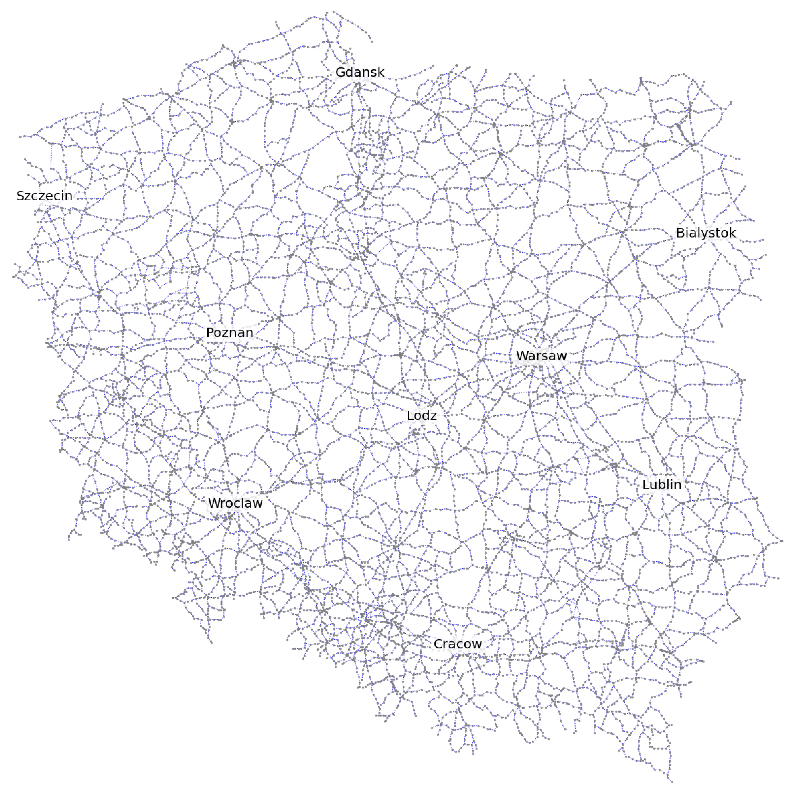
The model of the road transport network of Poland included 13,239 vertices and 15,010 edges. The implemented network included all the roads of national level; on the regional level, the network included voivodeship and powiat but not gmina roads.
A file with the nodes contained the codes of peculiar network nodes and the corresponding geographic coordinates.
The file with graph edge parameters contained the following data:
- Edge code;
- The codes of the output and input vertices (according to the codes defined in the file with vertex parameters);
- Length of the road network section (km);
- The number of lanes;
- Permissible speed in free movement (km/h);
- Road category;
- Results of traffic volume measurement according to the latest General Traffic Measurement (GTM 2015) for trucks and trucks with trailers (veh./day); if no traffic flow measurements were performed under GTM 2015, the relevant record contained the value None.
A graphical representation of the road transport network model created with the developed software is shown in Figure 1 (the visualization was created with the use of the networkx package tools).
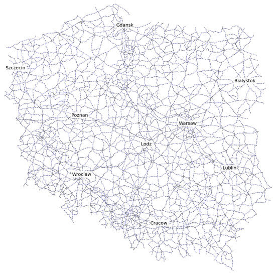
Figure 1.
Representation of the road network model of Poland created with the developed software.
The developed model of the road network was the basis for the next stages of the modeling process of the transport system for cargo deliveries by road transport in Poland.
3.2. Traffic Analysis Zones
Traffic analysis zones (TAZ) in the model of the country road transport system were adopted based on the current territorial division of the country into regions (the TERYT register). The total number of traffic analysis zones in the model was 2515.
For each TAZ, the center of gravity, the centroid, was determined in the transport system model. Centroids are defined in the model as graph vertices, they are connected to the transport network by connectors—virtual sections of the road network implemented as edges with zero numerical parameters. In the developed model of the transport system, the connectors are described based on a list of integer values that represent the codes of the network vertices closest in a straight line to the centroid.
The procedure for defining the centroid parameters for traffic analysis zones was developed in the form of a script. For this purpose, the specialized package OpenCage Geocoder (https://opencagedata.com, accessed on 8 July 2022) was used. For each TAZ, the GPS coordinates of its center of gravity were defined using the Geocoder functions. As input data, the prepared script used a file containing the names of traffic analysis zones and appropriate TERYT identifiers. The result of running the script was a file containing additionally the GPS coordinates for each of the centroids. At the next step of the simulation procedure, each of the centroids was attached by a connector to the nearest node of the network.
A graphic representation of the positions of the centroids for traffic analysis zones, estimated with the use of the developed script, is shown in Figure 2.
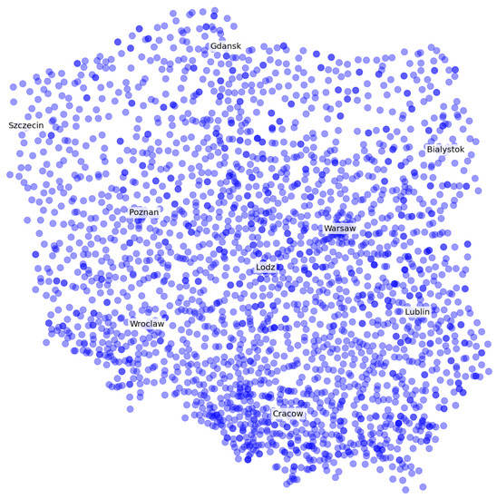
Figure 2.
Location of the centroid of traffic analysis zones in the model of the transport system.
3.3. Travel Demand Model
We proposed to shape the travel demand model based on the number of economic entities registered in each of the traffic analysis zones (according to the data of the Central Statistical Office of Poland) and based on the results of the TD-E survey allowing researchers to determine the traffic generated by economic entities depending on their type.
The TD-E survey is carried out by the Central Statistical Office of Poland each year. Randomly selected companies should obligatorily provide the information in the TD-E questionnaire about trips performed during the selected week of the year by all commercial vehicles owned by the company. The data must be reported for each day of the week the vehicle is operated and for each performed trip the following information should be provided: zip codes of the origin and destination regions, the distance covered, the consignment weight, the type of the cargo, and others.
The proposed methodology for building a transport demand model includes the following stages:
- Determination of the number of economic entities divided into groups according to the Polish Classification of Activities (PKA 2007) and according to the size of enterprises (large, medium, small) for each TAZ;
- Estimation of truck traffic generated by various types of economic units on an annual basis, separately for source traffic (trips aimed at exporting goods from the analyzed unit to other companies) and destination traffic (trips performed to deliver goods from other companies to the analyzed unit);
- Determination of the traffic-generating potential (production and attraction) of traffic analysis zones based on the records of business entities and data on truck traffic generated by each type of economic entity;
- Shaping the travel matrix (spatial distribution of travel–traffic patterns) based on the value of the mobility potential of traffic analysis zones.
The developed program script for shaping the database for the transport demand model contained the number of economic entities for various departments (according to the PKA 2007 classification–57 divisions: ‘01’, ‘02’, ‘03’, ‘05’, …, ‘81’, ‘82’) and various size of enterprises (large, medium, small) for each TAZ. As input data, the developed script used CSV files containing the number of enterprises for each class of PKA 2007 registered in the appropriate territorial unit (data on large, medium, and small enterprises were placed in separate files). The result of running the script was CSV files which contained for each TAZ the number of enterprises representing each division of the PKA 2007 classification; the results for enterprises of various sizes were presented in separate files.
3.3.1. Modeling the Demand for Domestic Trips
To estimate the average truck traffic generated by various types of economic units including the value of the traffic-generating potential, and shape the travel matrix, a script was developed in Python programming language. As input, the script used the following CSV files:
- Data on traffic analysis zones;
- Data on the number of business entities registered in individual traffic analysis zones (for large, medium, and small enterprises, respectively);
- Annual data from the TD-E questionnaires (this study analyzes data for 2018, the sample counts 151,532 records).
The result of the script execution was a CSV file containing the journey matrix.
The travel matrix is a square matrix of integer values: the rows of the matrix represent traffic analysis zones as origins of travel, and the columns of the matrix represent the zones of the destination. The elements of the travel matrix may also be floating-point values if the matrix represents the expected values of the number of performed trips.
The values of the travel matrix indicate the average number of trips made from the i-th to j-th TAZ. The diagonal elements of the travel matrix, located on the major diagonal, represent internal traffic inside the zones.
We propose to estimate the travel matrix elements based on the standard gravity model:
where:
is the production for the i-th TAZ,
is the attraction for the j-th TAZ,
is the value of the road resistance function (characterizing the distance or travel time between the i-th and the j-th TAZ),
is the total number of traffic analysis zones ().
The most common approach to defining the road resistance function is to use the inverse square value of the distance between the corresponding traffic analysis zones:
where:
is the shortest distance between the i-th and the j-th zones, estimated for the existing road network (km).
If the road resistance is not considered in a transport demand model, should be assumed for all pairs of i and j.
We propose to estimate the production and the attraction for the i-th territorial unit (territorial units in the model are identical to traffic analysis zones) based on the results of the TD-E survey as follows:
where:
, , and are the numbers of large, medium, and small enterprises of the k-th type registered in the i-th territorial unit,
, , and are the mean value of the number of annual inbound trips generated by the k-th type of large, medium, and small enterprises,
, , and are the average annual number of destination trips generated by the k-th type of large, medium, and small enterprises,
is the number of business unit types according to the PKA 2007 classification ().
As the sample containing the results of TD-E research did not include data on all categories and types of enterprises (for the sample from 2018, data were not available for 6 categories), some values for the average number of trips were approximated based on the data for other types of business entities. The values of the average annual number of source and destination trips for each of the considered types of business entities were estimated as the arithmetic mean values from samples containing the number of trips generated by enterprises of a given type (according to the results of the TD-E research). If the sample from the TD-E research did not contain data on enterprises of a certain type at all, the average number of trips generated by such enterprises was taken as a zero value. If the TD-E sample included data on trips generated by an enterprise of a certain type, but there were no data for enterprises of a certain size, the number of trips in this case was defined as the average of the number of trips for enterprises of other sizes (for which the data in the TD-E sample were available).
The total number of trips estimated using the presented methodology based on the 2018 TD-E research data amounted to approximately 11.4 million domestic trips per year.
The obtained travel matrix was one of the input parameters for the traffic flow estimation procedures on the given sections of the road network and the estimation of transport performance for the traffic analysis zones.
3.3.2. Modeling the Demand for Foreign Trips
We proposed to simulate the international truck traffic for each traffic analysis zone based on the number of companies registered in the corresponding zones and data on the number of foreign trips obtained from the TD-E sample.
The total number of records containing data on foreign trips in the TD-E sample for 2018 was 9669. These were trips made by Polish enterprises for the delivery of goods both from abroad to the country (a total of 4811 trips) and from Poland to foreign countries (a total of 4858 trips). Each record in the data file contained the company ID in the sample, the code of the type of activity performed according to the PKA 2007 classifier, the codes of the loading and unloading countries, and the weight of the loaded and unloaded goods in kilograms.
To analyze data on foreign travels, a Python script was developed, the launch of which yielded a file containing the results of estimating the average values of the number of foreign trips from and to the country performed annually by enterprises registered in each of the traffic analysis zones.
As the sample with TD-E survey results for 2018 contained data on foreign travel only for 4414 enterprises, it was not possible to provide the level of detail with the accuracy to the division according to PKA 2007 (this level of detail was adopted in the methodology of estimating domestic travel matrix) in the case of modeling foreign travel: based on the analyzed TD-E sample, it was possible to estimate the average values of the number of trips performed annually for only 39 out of 57 divisions of the classifier. Therefore, the assessment of the number of foreign trips was performed with the accuracy of the PKA 2007 section (sections A, B, C, D, E, F, G, H, K, N). The division of enterprises into types according to size was also not considered.
For each trip in the analyzed sample, the country whose border with Poland was crossed was defined based on the assumptions presented in Table 1.

Table 1.
Assumptions about crossing borders when making a trip.
The travel demand model assumed that the trip was made to (or from) the country the border of which the vehicle crossed when leaving Poland (or entering Poland). The locations of border crossings included in the model of the road transport system of Poland are shown in Figure 3.
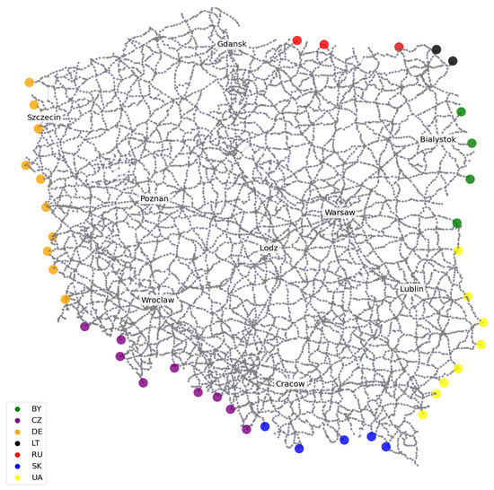
Figure 3.
Location of border crossings on the road transport network of Poland.
Neighboring countries in the simulation model are shown as traffic analysis zones whose centroids are connected by zero-length edges to each of the vertices representing the respective border crossings. In the model of the transport system, the traffic-generating potential of the given traffic analysis zones represented the demand for freight transport in the appropriate direction.
Based on the results of the analysis of the TD-E survey data, the average annual number of foreign trips for the i-th TAZ in the j-th direction was proposed to be estimated in the following way:
where:
, , and are the numbers of large, medium, and small enterprises of the k-th type registered in the i-th territorial unit,
is the empirically obtained number of foreign trips (based on the TD-E sample) performed by the k-th type enterprises in the j-th direction,
is the part of the enterprises of the k-th type in the TD-E sample,
stands for travels from abroad to Poland, is the notation for travel from Poland to abroad,
is the number of types of companies divided into sections according to the PKA 2007 classification ().
According to the results of the calculations based on the TD-E sample for 2018, the total number of trips from abroad to Poland was approximately 1498 thousand, and the total number of journeys from Poland to abroad was approximately 1564 thousand.
The foreign travel matrix obtained based on the presented methodology was an input parameter for the procedures of the traffic volume and the transport performance estimations.
3.4. Distribution of Trips on the Road Network
We proposed to perform the distribution of trips in the network using the following sequence:
- Determination of travel paths in the transport network for each pair of traffic analysis zones, except for pairs for which the travel matrix element was a zero value;
- Estimation of the load on each of the sections of the road network (graph edges) based on the generated travel paths.
The determination of the travel paths was performed based on the Dijkstra algorithm.
Determining the paths was the most time-consuming computational procedure in the proposed methodology. For each TAZ, the shortest paths to the remaining zones were reconstructed based on the auxiliary vector (the number of vector elements was equal to the number of vertices of the transport network), whose elements indicate the codes of the vertices on the shortest path. For the road transport network of Poland, the procedure of calculating the auxiliary vector based on the Dijkstra algorithm for one TAZ took about 3 min (i7 processor, 32 GB RAM), and for all 2515 zones about 126 h. Even after the computation time was reduced as the result of the parallel computation algorithm, the total shortest distance matrix estimation time was about 18 h (i7 processor, 8 cores, 32 GB RAM). This is an unsatisfactory result for performing the calculations in real-world conditions.
To use the developed model in practice and to avoid time-consuming calculations, we recommend preparing text files containing vectors for path reconstruction beforehand. The total size of the files for shaping the shortest paths for all traffic analysis zones of Poland was 172 MB. The procedure of distribution of trips on the road network for a set of all territorial regions of the country performed based on previously prepared files with auxiliary vectors took about 20 min on a computer with an i7 processor and 32 GB of RAM.
4. Software Implementation
The developed software for simulation of a road transport system included the following basic classes:
- Node: a vertex of the graph as a component of the transport network model;
- Link: an edge of the graph in the network model;
- Net: a transport network;
- TSModel: a model of the transport system.
The structure of the developed base classes in the form of a UML diagram is presented in Figure 4.
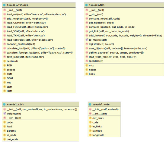
Figure 4.
UML-diagram library for road transport system modeling.
The Node class fields characterize the network vertices according to the presented mathematical model of the transport network:
- code: an integer value representing the unique vertex code;
- latitude and longitude: floating-point values, geographical coordinates;
- out_links and in_links: collections of the Link type elements that represent sets of exit edges (for which the vertex is the source point) and entry edges (for which the vertex is the destination point).
The Link class objects are characterized based on the following fields:
- code: an integer value, the unique edge code;
- out_node and in_node: the references to the Node objects that point to the starting and ending vertices of the edge;
- load: a floating-point value that characterizes the edge load (traffic volume);
- params: a list of additional numerical parameters characterizing the edge; the first element of this list is the weight of the edge (e.g., length of a net section).
The Net class has the following internal fields:
- nodes: a list of the Node objects, a set of all network nodes;
- links: a list of the Link objects, a set of all network edges;
- mtx: a square matrix of floating-point values, the size of the matrix is equal to the number of nodes in the network; the matrix elements contain the weight of the edge connecting the corresponding vertices, or None if the graph nodes are not connected by an edge.
The algorithms for modeling the transport network are implemented as methods of the Net class:
- load_from_file: reads network configuration from CSV files containing data about vertices and edges;
- recode: sorts all network nodes (the nodes list elements) according to their unique code in ascending order and assigns new codes starting from 0;
- add_link: adds a new edge (an object of the Link type) to the links list;
- get_link: returns the first found link in the links list with the source and target nodes given as the method arguments, or None if the links list does not contain edges with the given parameters;
- contains_link: returns True if the links list contains an element with source and destination nodes given as method arguments, otherwise returns False;
- get_node: returns the first found element of the nodes list, the unique code of which corresponds to the value given as an argument of the method, or None, if the nodes list does not contain an element with the given code;
- contains_node: returns True if the nodes list contains an element with the unique code given as a method argument, or returns False otherwise;
- dijkstra: implements the Dijkstra algorithm, returns a list of integer values; the number of list elements is equal to the number of nodes in the network; the list items represent the unique codes of the network nodes along which the shortest path runs; the method parameters is the Node object representing the source vertex for which the shortest paths to the remaining vertices should be defined;
- save_dijkstra: writes vectors to the CSV file to retrieve the shortest paths for a vertices list given as an argument of the method;
- define_path: retrieves the shortest path between a pair of vertices given as the method arguments; the method returns a list of the Node elements whose order represents the shortest path.
The proposed approach to modeling the road transport system is implemented in the TSModel class. The fields of the TSModel class represent the basic elements of the model:
- net: the Net class object representing the transport network;
- centroids: a dictionary containing data on centroids, in which the TERYT code of the TAZ is the key, and the value—a tuple with the geographic coordinates of the centroids;
- ccodes: a list of integer values representing the unique codes of the vertices of the transport network located closest to the corresponding centroid;
- SDM: a square matrix of floating-point values; the size of the matrix is equal to the number of traffic analysis zones, where the elements of the matrix represent the shortest distances between the corresponding pair of zones;
- ODM: a square matrix of floating-point values; the size of the matrix is equal to the number of traffic analysis zones; the matrix elements represent the average number of trips performed annually between a pair of corresponding zones;
- FOM and FDM: matrices of floating-point values, the number of rows of each matrix is equal to the number of traffic analysis zones, the number of columns of the matrices is equal to the number of countries with which Poland has a common land border, the elements of the matrix are the average number of trips made annually from Poland to its neighbors (FOM matrix) and from neighboring countries to Poland (FDM matrix);
- TKM: a square matrix of floating-point values, the size of the matrix is equal to the number of traffic analysis zones, the matrix elements represent the average transport performance in ton-kilometers per year for the delivery of goods between a pair of respective zones.
Transport network model elements can be loaded into fields of the TSModel instances using the following methods:
- load_net: reads the transport network configuration from CSV files to the net field;
- load_centroids: reads from the CSV file into the centroids field centroid coordinates for each of the traffic analysis zones;
- load_SDM: reads the shortest distance matrix values from the CSV file into the SDM field;
- add_neighbors: adds to the network model the traffic analysis zones representing the countries with which Poland has a common land border; data on neighboring countries are given as an argument of the method in the form of a dictionary, where the dictionary key represents the name of the country and the value is a tuple, the first element of which is a tuple with region coordinates, and the second a list of network vertex codes representing the relevant border crossings.
Demand model elements are loaded using the following methods:
- laod_ODM: reads the values of the elements of the origin-destination matrix from the CSV file into the ODM field;
- load_FODM: loads the average number of foreign trips from the CSV file to the FOM and the FDM fields;
- load_TKM: loads from the CSV file into the TKM field the data on the performed transport work.
The developed transport system modeling procedures are presented by the following TSModel class methods:
- connect_centriods: connects the centroids of traffic analysis zones to the transport network by defining the value of the ccodes field;
- calculate_load: calculates a load of network sections for domestic services based on the traffic distribution and vectors for retrieving the shortest paths; vectors are read from CSV files, the list of which is given as an argument to the method;
- calculate_foreign_load: calculates the load on network sections for international transport based on the foreign traffic matrix and vectors for retrieving the shortest paths; vectors are read from the CSV file given as an argument of the method.
As part of the TSModel class, the save_load method has also been implemented, which allows saving the load on the road network to a CSV file provided as an argument of the method. The output file records contain the source and destination node codes for each edge and the annual average traffic flow of the corresponding network segment.
5. Simulation Results and Discussion
The traffic volume on individual sections of the road network was estimated based on the results of launching the procedure for distributing performed trips to the transport network. For the j-th section of the road network, the volume of commercial vehicle traffic was defined as the number of all trips for which the shortest path included a given network section.
The travel path between the i-th and the j-th traffic analysis zones can be defined as the vector of length (the number of edges in the graph-model of the transport network), whereby each element of this vector is a zero-one variable:
, ,
.
Then, the traffic volume on the k-th section of the road network can be estimated using the following formula:
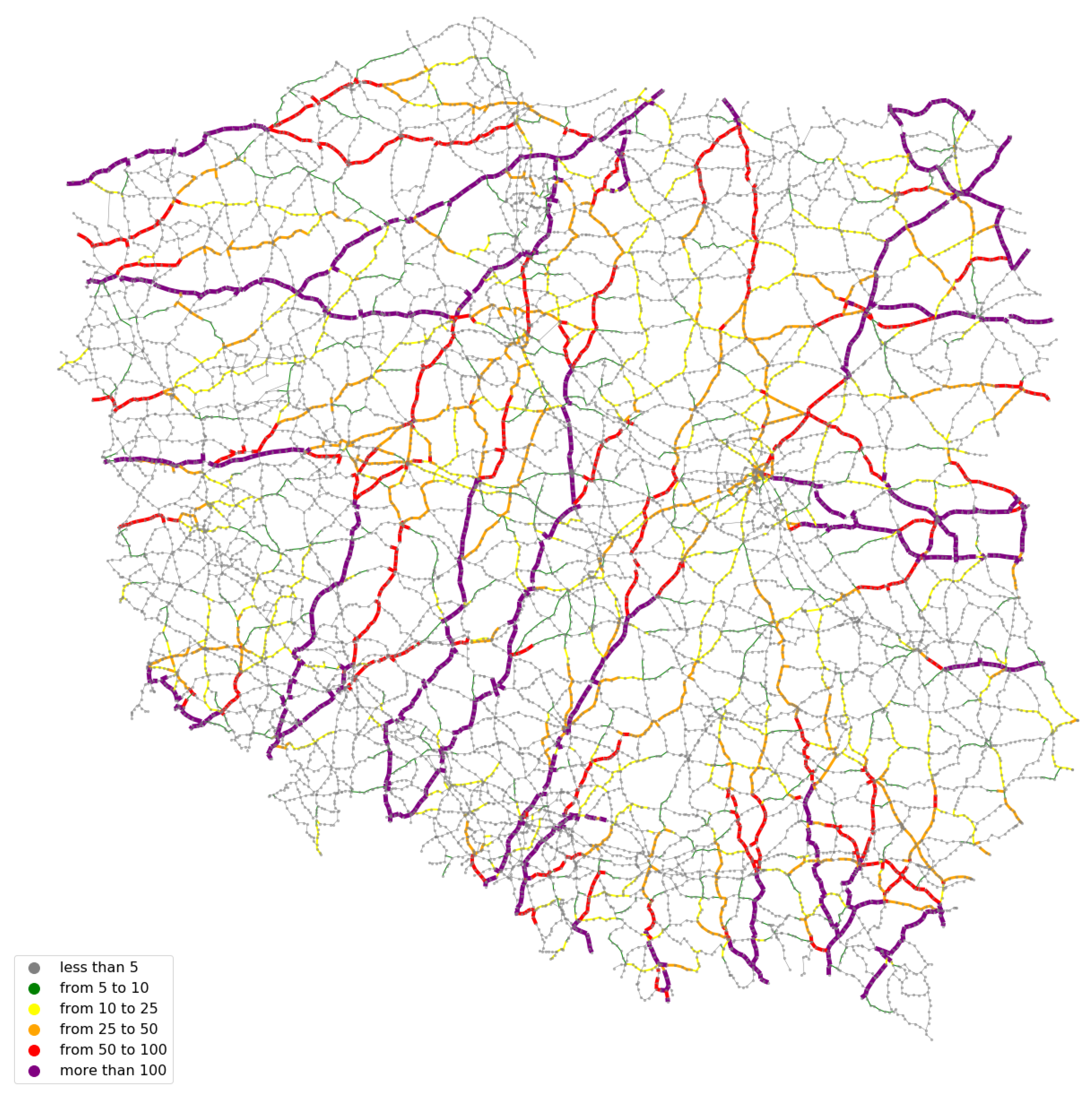
The results of the assessment of the traffic flows generated by foreign trips obtained based on the developed model of the road transport system and with the use of the TD-E data from 2018 are presented in Figure 5.
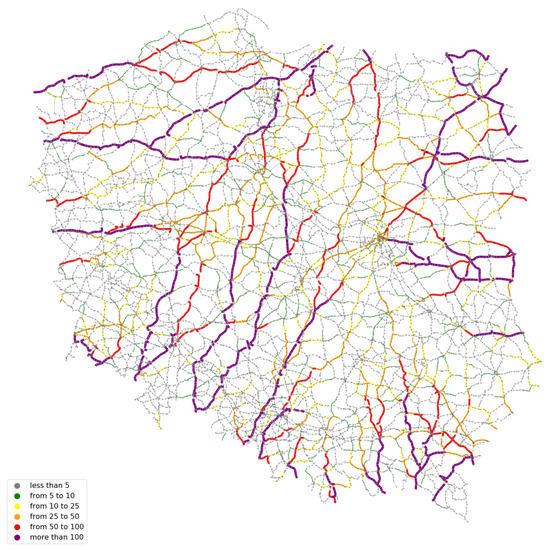
Figure 5.
Traffic volume assessment results for foreign trips.
The parameters of the sample representing the traffic flows generated by foreign trips are included in Table 2.

Table 2.
Sample structure of traffic volumes generated by travels abroad.
The corresponding results for the traffic flows generated by domestic trips are presented in Figure 6 and Table 3.
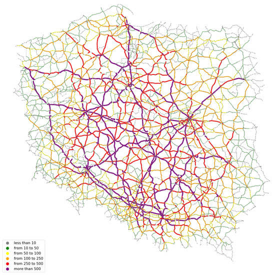
Figure 6.
Results of the assessment of traffic volumes for domestic trips.

Table 3.
Sample structure of traffic volumes generated by domestic trips.
The results of modeling the traffic volume generated jointly by domestic and foreign trips are presented in Figure 7 and Table 4.
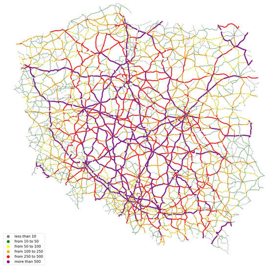
Figure 7.
Traffic volume assessment results for domestic and foreign trips jointly.

Table 4.
The structure of the sample of traffic flows generated jointly by domestic and foreign trips.
We proposed to estimate the adequacy of the developed model of the country’s road transport system by using the determination coefficient for the set of freight traffic flows on selected sections of the road network and the corresponding set of traffic flows, the values of which were obtained empirically as the result of direct counts:
where:
and are theoretical (simulated) and empirical (observed in field studies) traffic volumes on the i-th section of the road network (veh./day);
is the arithmetic mean value of traffic flow from the set of empirical values (veh./day);
is the number of road network sections where traffic volume measurements were carried out during field studies.
For macro-models of transport systems, the results of simulations were satisfactory if the value of the coefficient was above 0.6.
The results of the latest General Traffic Measurement (GTM 2015) were used as the reference values to estimate the adequacy of the obtained model. The GTM 2015 survey covered 88.7% of all sections of the road network (average daily traffic volume was estimated for 13,315 sections out of 15,010 road network sections). The visualization of the empirical results of the traffic volumes’ measurements is shown in Figure 8. The structure characteristics for the sample of empirical traffic flows are presented in Table 5.
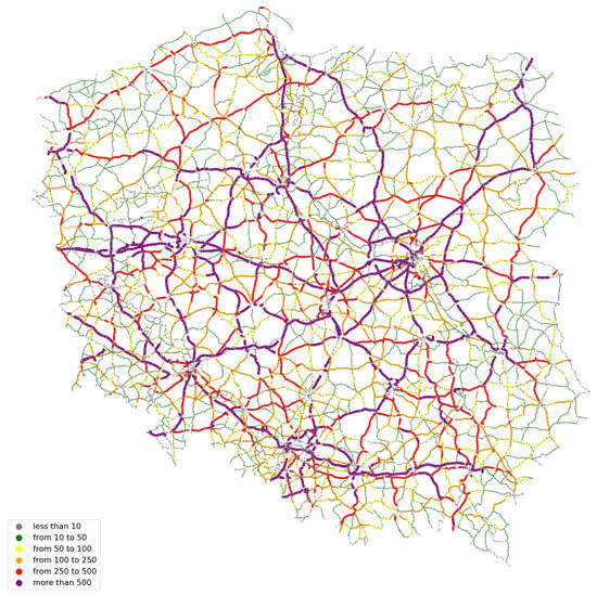
Figure 8.
Traffic volumes on the road network according to GTM 2015.

Table 5.
Structure of the traffic volumes sample from GTM 2015.
The comparison of the theoretical values of the volumes of freight traffic generated jointly by domestic and foreign trips with the appropriate empirical values was carried out for a set of those network sections where the empirical values were determined with GTM 2015 studies. The value of the coefficient of determination, calculated for the empirical traffic volumes obtained as the result of the GTM 2015 and the traffic volumes estimated based on the developed model, was 0.62, which proved a satisfactory fit and the adequacy of the obtained model.
For each of the examined road network sections, the absolute model error was estimated additionally in the following way:
If the absolute model error for the i-th segment was , then the degree of model fit for this segment was at the level .
The road sections with a fit greater than 95% are shown in Figure 9.
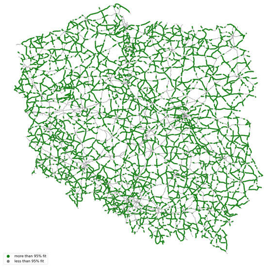
Figure 9.
Sections of the road network with a degree of matching above 95%.
The results of the absolute model error assessment show that the average error for all checked network sections was 10.34%.
Among all empirically tested sections, we identified the sections for which the model error was lower than 5% (or the degree of fit was above 95%). The share of the sections with the degree of matching above 95% was 48%, and the average absolute error for these sections was 1.93%.
To characterize the elements with an unsatisfactory fit, the sections for which the model error was above 50% (or the degree of matching was lower than 50%) were defined among all empirically tested sections of the road network. The share of sections with an unsatisfactory fit in the set of all examined sections was 2.78%. The mean absolute error for the sections with an unsatisfactory fit was 62.13%.
The road sections with less than 50% match are shown in Figure 10.
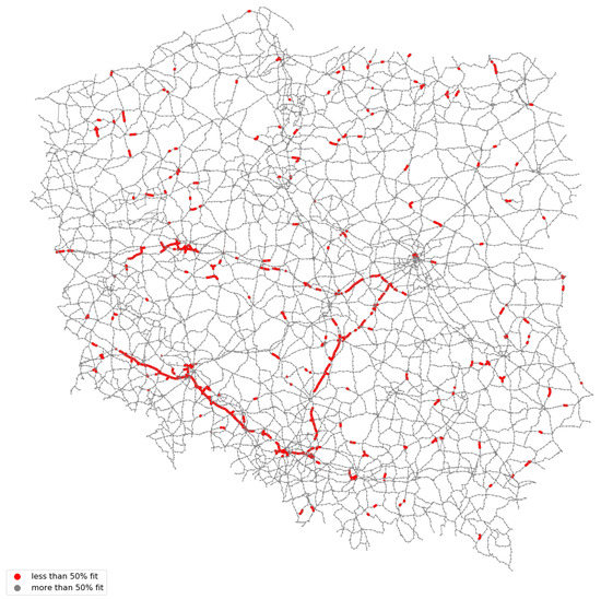
Figure 10.
Sections of the road network with a degree of matching below 50%.
6. Conclusions
The proposed methodology for modeling heavy road transport is based on representative data used in demand modeling procedures, which allows avoiding the use of time-consuming heuristics to stimulate demand based on econometric models. The resulting model of the transport system is characterized by satisfactory adequacy, which can be improved after using more advanced techniques for calibrating the model parameters.
An advantage of the developed approach is the use of open-source software, without the use of commercial tools. This enables the use of the proposed methodology by the Central Statistical Office of Poland to estimate the transportation work generated by the traffic analysis zones and to forecast the average traffic volume on selected sections of the country’s road network.
The significant limitation of the approach to model freight road transport based on the TD-E survey is the lack of data about transit trips—freight deliveries through the territory of Poland with the origin and the destination in other countries. As the TD-E survey does not consider trips that start and finish in foreign countries, a demand model developed with the proposed approach will be not complete. However, that does not have a significant influence on the simulation results, as that part of the transit road traffic, according to the Central Statistical Office of Poland, is less than 5% of the total volume of freight traffic.
Another limitation of the proposed methodology is related to the scale of the transport system: as the model was created at the macro scale, the characteristics of the trips were simplified and unified—we did not consider the type of transported cargo, the type of the used vehicle, routing and scheduling procedures, etc.
In further studies on improving the obtained model, we plan to refactor the traffic distribution algorithm by defining paths based on travel time and to improve the efficiency of the algorithm for determining the shortest paths by implementing procedures for parallel calculations.
Author Contributions
Conceptualization, V.N. and A.S.; methodology, V.N. and A.S.; software, V.N. and H.V.; validation, V.N. and H.V.; formal analysis, V.N.; investigation, V.N., A.S. and H.V.; resources, A.S.; data curation, V.N. and H.V.; writing—original draft preparation, V.N. and H.V.; writing—review and editing, A.S.; visualization, V.N.; project administration, A.S. All authors have read and agreed to the published version of the manuscript.
Funding
This research was carried out in the frame of the project: “Intelligent system for the production of road and maritime transport statistics with the use of large volumes of data to shape the country’s transport policy” under the Strategic Program of Scientific Research and Development “Social and economic development of Poland in the conditions of globalizing markets” GOSPOSTRATEG. The publication was funded as part of the project “ROAD TO EXCELLENCE—a comprehensive university support program”, implemented under the Operational Program Knowledge Education Development 2014–2020, co-financed by the European Social Fund; agreement No. POWR.03.05.00-00-Z214/18.
Institutional Review Board Statement
Not applicable.
Informed Consent Statement
Not applicable.
Conflicts of Interest
The authors declare no conflict of interest.
References
- Cascetta, E. Transportation Systems Analysis. Models and Applications, 2nd ed.; Springer: New York, NY, USA, 2009. [Google Scholar] [CrossRef]
- De Dios Ortúzar, J.; Willumsen, L.G. Modelling Transport, 4th ed.; John Wiley & Sons: Hoboken, NJ, USA, 2011. [Google Scholar] [CrossRef]
- Janić, M. Transport Systems: Modelling, Planning, and Evaluation, 1st ed.; CRC Press: Boca Raton, FL, USA, 2017. [Google Scholar] [CrossRef]
- Khalili, S.; Rantanen, E.; Bogdanov, D.; Breyer, C. Global transportation demand development with impacts on the energy demand and greenhouse gas emissions in a climate-constrained world. Energies 2019, 12, 3870. [Google Scholar] [CrossRef] [Green Version]
- de Blas, I.; Mediavilla, M.; Capellán-Pérez, I.; Duce, C. The limits of transport decarbonization under the current growth paradigm. Energy Strategy Rev. 2020, 32, 100543. [Google Scholar] [CrossRef]
- Profillidis, V.A.; Botzoris, G.N. Modeling of Transport Demand: Analyzing, Calculating, and Forecasting Transport Demand, 1st ed.; Elsevier: Amsterdam, The Netherlands, 2018. [Google Scholar] [CrossRef]
- Le Pira, M.; Inturri, G.; Ignaccolo, M. Modeling and simulation for transport planning. In International Encyclopedia of Transportation; Vickerman, R., Ed.; Elsevier: Amsterdam, The Netherlands, 2021; pp. 184–190. [Google Scholar] [CrossRef]
- Tang, C.K.; Zhang, L. Principles and Practices of Transportation Planning and Engineering, 1st ed.; CRC Press: Boca Raton, FL, USA, 2021. [Google Scholar] [CrossRef]
- Kłos, M.J.; Sobota, A.; Żochowska, R.; Soczówka, P. Traffic measurements for development a transport model. Adv. Intell. Syst. Comput. 2020, 1091, 265–278. [Google Scholar] [CrossRef]
- Meersman, H.; van de Voorde, E. Freight transport models: Ready to support transport policy of the future? Transp. Policy 2019, 83, 97–101. [Google Scholar] [CrossRef]
- Ewing, R.; Sabouri, S.; Park, K.; Lyons, T.; Tian, G. Key Enhancements to the WFRC/MAG Four-Step Travel Demand Model; Transportation Research and Education Center (TREC): Portland, OR, USA, 2019. [Google Scholar] [CrossRef]
- Park, K.; Sabouri, S.; Lyons, T.; Tian, G.; Ewing, R. Intrazonal or interzonal? Improving intrazonal travel forecast in a four-step travel demand model. Transportation 2020, 47, 2087–2108. [Google Scholar] [CrossRef]
- Saberi, M.; Rashidi, T.H.; Ghasri, M.; Ewe, K. A complex network methodology for travel demand model evaluation and validation. Netw. Spat. Econ. 2018, 18, 1051–1073. [Google Scholar] [CrossRef]
- Apronti, D.T.; Ksaibati, K. Four-step travel demand model implementation for estimating traffic volumes on rural low-volume roads in Wyoming. Transp. Plan. Technol. 2018, 41, 557–571. [Google Scholar] [CrossRef]
- Horváth, M.T.; Mátrai, T.; Tóth, J. Route planning methodology with four-step model and dynamic assignments. Transp. Res. Procedia 2017, 27, 1017–1025. [Google Scholar] [CrossRef]
- Hartleb, J.; Friedrich, M.; Richter, E. Vehicle scheduling for on-demand vehicle fleets in macroscopic travel demand models. Transportation 2021, 1172, 1–23. [Google Scholar] [CrossRef]
- Wörle, T.; Briem, L.; Heilig, M.; Kagerbauer, M.; Vortisch, P. Modeling intermodal travel behavior in an agent-based travel demand model. Procedia Comput. Sci. 2021, 184, 202–209. [Google Scholar] [CrossRef]
- Croce, A.I.; Musolino, G.; Rindone, C.; Vitetta, A. Estimation of travel demand models with limited information: Floating car data for parameters’ calibration. Sustainability 2021, 13, 8838. [Google Scholar] [CrossRef]
- Reiffer, A.; Heilig, M.; Kagerbauer, M.; Vortisch, P. Microscopic demand modeling of urban and regional commercial transport. Procedia Comput. Sci. 2018, 130, 667–674. [Google Scholar] [CrossRef]
- Naumov, V.; Szarata, A.; Vasiutina, H. A Methodological approach to the real-time data analysis from the ViaTOLL system. Lect. Notes Netw. Syst. 2021, 208, 115–128. [Google Scholar] [CrossRef]
- Storani, F.; Di Pace, R.; Bruno, F.; Fiori, C. Analysis and comparison of traffic flow models: A new hybrid traffic flow model vs benchmark models. Eur. Transp. Res. Rev. 2021, 13, 58. [Google Scholar] [CrossRef]
- Möller, D.P.F. Introduction to Transportation Analysis, Modeling and Simulation; Springer: London, UK, 2014. [Google Scholar] [CrossRef]
- Pell, A.; Meingast, A.; Schauer, O. Trends in real-time traffic simulation. Transp. Res. Procedia 2017, 25, 1477–1484. [Google Scholar] [CrossRef]
- Ejercito, P.M.; Nebrija, K.G.E.; Feria, R.P.; Lara-Figueroa, L.L. Traffic simulation software review. In Proceedings of the 8th International Conference on Information, Intelligence, Systems & Applications (IISA), Larnaca, Cyprus, 27–30 August 2017; pp. 1–4. [Google Scholar] [CrossRef]
- Janczykowski, M.; Turek, W.; Malawski, M.; Byrski, A. Large-scale urban traffic simulation with Scala and high-performance computing system. J. Comput. Sci. 2019, 35, 91–101. [Google Scholar] [CrossRef]
- Stinson, M.; Auld, J.; Mohammadian, A. A large-scale, agent-based simulation of metropolitan freight movements with passenger and freight market interactions. Procedia Comput. Sci. 2020, 170, 771–778. [Google Scholar] [CrossRef]
- Gonzalez-Delicado, J.J.; Gozalvez, J.; Mena-Oreja, J.; Sepulcre, M.; Coll-Perales, B. Alicante-Murcia freeway scenario: A high-accuracy and large-scale traffic simulation scenario generated using a novel traffic demand calibration method in SUMO. IEEE Access 2021, 9, 154423–154434. [Google Scholar] [CrossRef]
- Codeca, L.; Frank, R.; Faye, S.; Engel, T. Luxembourg SUMO Traffic (LuST) scenario: Traffic demand evaluation. IEEE Intell. Transp. Syst. Mag. 2017, 9, 52–63. [Google Scholar] [CrossRef]
- Manser, P.; Becker, H.; Hörl, S.; Axhausen, K.W. Designing a large-scale public transport network using agent-based microsimulation. Transp. Res. Part A Policy Pract. 2020, 137, 1–15. [Google Scholar] [CrossRef]
- Thonhofer, E.; Palau, T.; Kuhn, A.; Jakubek, S.; Kozek, M. Macroscopic traffic model for large scale urban traffic network design. Simul. Model. Pract. Theory 2018, 80, 32–49. [Google Scholar] [CrossRef]
- Liu, Y.; Lyu, C.; Zhang, Y.; Liu, Z.; Yu, W.; Qu, X. DeepTSP: Deep traffic state prediction model based on large-scale empirical data. Commun. Transp. Res. 2021, 1, 100012. [Google Scholar] [CrossRef]
- Lopez-Martin, M.; Carro, B.; Sanchez-Esguevillas, A. Neural network architecture based on gradient boosting for IoT traffic prediction. Future Gener. Comput. Syst. 2019, 100, 656–673. [Google Scholar] [CrossRef]
- Chen, Y.-T.; Sun, E.W.; Chang, M.-F.; Lin, Y.-B. Pragmatic real-time logistics management with traffic IoT infrastructure: Big data predictive analytics of freight travel time for Logistics 4.0. Int. J. Prod. Econ. 2021, 238, 108157. [Google Scholar] [CrossRef]
- Sonnleitner, J.; Friedrich, M.; Richter, E. Impacts of highly automated vehicles on travel demand: Macroscopic modeling methods and some results. Transportation 2022, 49, 927–950. [Google Scholar] [CrossRef]
- Baalsrud Hauge, J.; Ramos Carretero, M.; Kodjabachian, J.; Meijer, S.; Raghothama, J.; Duqueroie, B. ProtoWorld—A simulation based gaming environment to model and plan urban mobility. Lect. Notes Comput. Sci. 2016, 9599, 393–400. [Google Scholar] [CrossRef]
- Anand, N.; Meijer, D.; van Duin, J.H.R.; Tavasszy, L.; Meijer, S. Validation of an agent based model using a participatory simulation gaming approach: The case of city logistics. Transp. Res. Part C Emerg. Technol. 2016, 71, 489–499. [Google Scholar] [CrossRef]
Publisher’s Note: MDPI stays neutral with regard to jurisdictional claims in published maps and institutional affiliations. |
© 2022 by the authors. Licensee MDPI, Basel, Switzerland. This article is an open access article distributed under the terms and conditions of the Creative Commons Attribution (CC BY) license (https://creativecommons.org/licenses/by/4.0/).

