Computational Fluid Dynamics Simulation Approach for Scrubber Wash Water pH Modelling

Abstract

In the current article, we will use a CFD approach for the scrubber wash water dilution simulation, by considering the current MEPC (Marine Environment Protection Committee, a subsidiary of IMO—International Maritime Organization) regulations that are in force. The necessity for scrubber wash water pH modelling and its importance in the current environmental framework is emphasized. The presented 3D model is considered as a 400 mm hydraulic diameter fluid domain with two outlets and a discharge water flow rate of 3050 m³/h for the considered pH value of 3, obtained within a state-of-the-art exhaust gas scrubber solution developed by a major EGCS (Exhaust Gas Cleaning Systems) supplier. The CFD study was developed by considering a k-ε turbulence model. In order to achieve accurate results, a structured mesh with two levels of refinement volumes was realized. Based on the obtained data and the various parameters discussed, the paper presents a way to investigate the optimal results for further analytical research of the scrubber washwater dilution process within the exhaust gas cleaning system.

1. Introduction

Within the shipping industry, large quantities of fossil fuels are burned by the ship’s diesel engines, with the exhaust gases having carbon oxides (CO_x) and water (H₂O) as the main components. Together with the main fractions [1,2,3], the combustion process also generates sulfur oxides (SO_x), nitrogen oxides (NO_x), and carbon-based matter (soot, smoke), all of them with huge environmental impact, such as acid rain and carbon-based airborne particles, which are detrimental to human health.

Based on the real global concern about environmental issues, determined by the exhaust gas emissions and their impact, there is a huge interest in developing technical solutions for reducing the level of pollution [4,5,6,7].

Therefore, for both new builds and existing ships, a fitting/retrofitting race is ongoing—increasingly ships are using various solutions for cleaning the exhaust gases. A scrubber technology was developed with unique features to enable a more sustainable operating environment for the shipping industry [8].

The main objective of this study is to evaluate the open-loop solution, with an emphasis on the aspects regulated within MEPC 259(68).

The open-loop cleaning process is based on exhaust gases “washing” with seawater, thus resulting in large quantities of residuals—sulfuric acid (H₂SO₄) or sulfurous acid (H₂SO₃) diluted in the wash water. The obtained product is seawater with increased acidity, which is to be discharged overboard (either treated in a second stage or diluted).

2. Study Aim, Materials and Methods

2.1. Marine Environment and Seawater Alkalinity

The wash water with low pH values reacts with the salt in the seawater, forming carbonic acid, which is considered to be unharmful for the marine environment. The main source of hydrogen ions (H⁺) absorbents in the seawater is formed by the carbonate and bicarbonate salts naturally present [8,9,10]. The natural presence of the salts generates an alkaline seawater. The general values of seawater alkalinity around the globe range from 2200–2400 µmol/kg.

Nevertheless, diluted sulfuric acid from the wash water is a threat to the marine environment and, therefore, additional rules are required in order to create the lowest possible environmental impact due to ship wash water discharge.

Guidelines for exhaust gas cleaning systems, applicable for this study, are published in the Resolution MEPC.259(68) in Annex 1 and are stated as follows: 10.1.2.1. “The pH discharge limit, at the overboard monitoring position, is the value that will achieve as a minimum pH 6.5 at 4 m from the overboard discharge point with the ship stationary”.

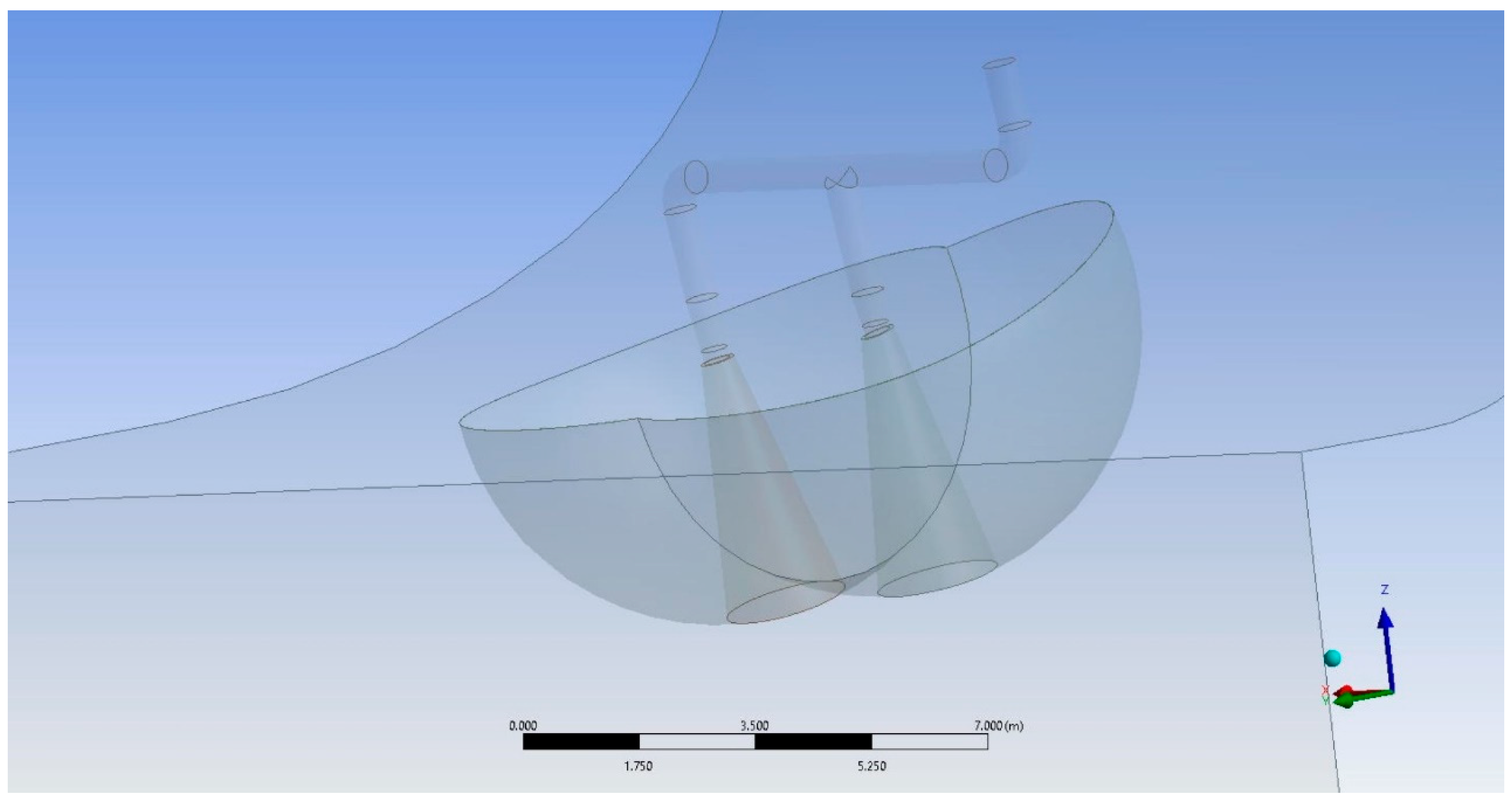
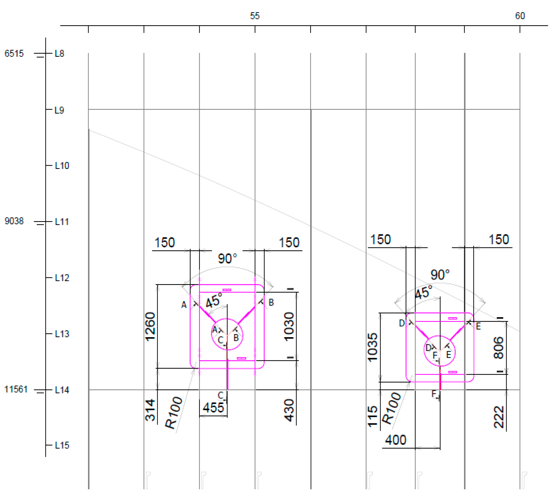
2.2. Main Parameters and Initial Setup Geometry

The study assesses the compliance with MEPC 259(68) paragraph 10.1.2.1 and relevant DNV-GL (Det Norske Veritas) and BV (Bureau Veritas) rules and regulations for the ship wash water discharge.

Based on existing references, a computational model was created that takes into account the existing rules and the specific functional status of the ship’s propulsion and power generation systems [11,12].

The starting point for the initial setup geometry is presented in Figure 1. For the simulation in CFD, all elements designed for enhancing the flow turbulence were removed and the scrubber wash water inlet surface was assigned to be at 1 m distance from the outlet piping elbow.

In this way, the simulation is developed with a conservative approach, starting with the geometry setup, by decreasing the turbulence values affected by the existing valves or piping elements. This objective, of achieving the most conservative approach, is accomplished by decreasing the dilution quality obtained when using such turbulence-enhancing attachments.

The simulation setup is developed using the following initial operational setup:

• Seawater temperature: 25 °C;
• Discharge water temperature: 35 °C;
• Discharge water flow rate: 3050 m³/h—considered to be the flow at full load while the ship is stationary;
• Number of outlets: 2;
• Discharge water pH: 3;
• Considered ship speed: 0 kn (stationary).

To assess the dilution pattern in the initial setup, the hull geometry of a ship that actually has the system onboard is used [13,14]. To reduce the influence of turbulence in the numerical analysis, all diffusers and turbulence-increasing elements were removed (for example, all valves on the terminal line of the scrubber wash water outlet were disregarded).

For a proper assessment of the dilution pattern, at the required 4 m distance from the outlets, there were used two spherical volumes, with a radius of 4 m and the center in the outlet center (Figure 1). In the same figure, we can observe the intersection of the two spherical volumes with the ship hull and the position of the scrubber outlet shell penetrations [15,16].

The outlet location is identified based on the penetration plan, as presented in Figure 2.

The generated geometry (Figure 1) follows the position and dimensions stated in the construction drawings, available during the retrofit project of the ship which was the subject of certification (Figure 2).

The bounding box of the computational domain for scrubber wash water pH modelling has the following dimensions: Height = 20 m, Width = 35 m, Length = 60 m.

The origin of the coordinate system is located on the ship hull surface, the Ox axis positive toward fore, the Oy axis positive toward portside, and the Oz axis positive upwards [17]. For boundaries definition, the details identified in the initial setup geometry are as shown in Figure 3.

The computational domain was simplified as shown in Figure 3, by taking into account the following aspects:

• The need to decrease the computational effort leads to the model being generated to consider only the hull section in the area of interest.
• Since the main requirement is to have no flow around the hull, without any current alongside [13,14,15,16,17], it is reasonable to assume that there will also be no wash water flow in the hull proximity.

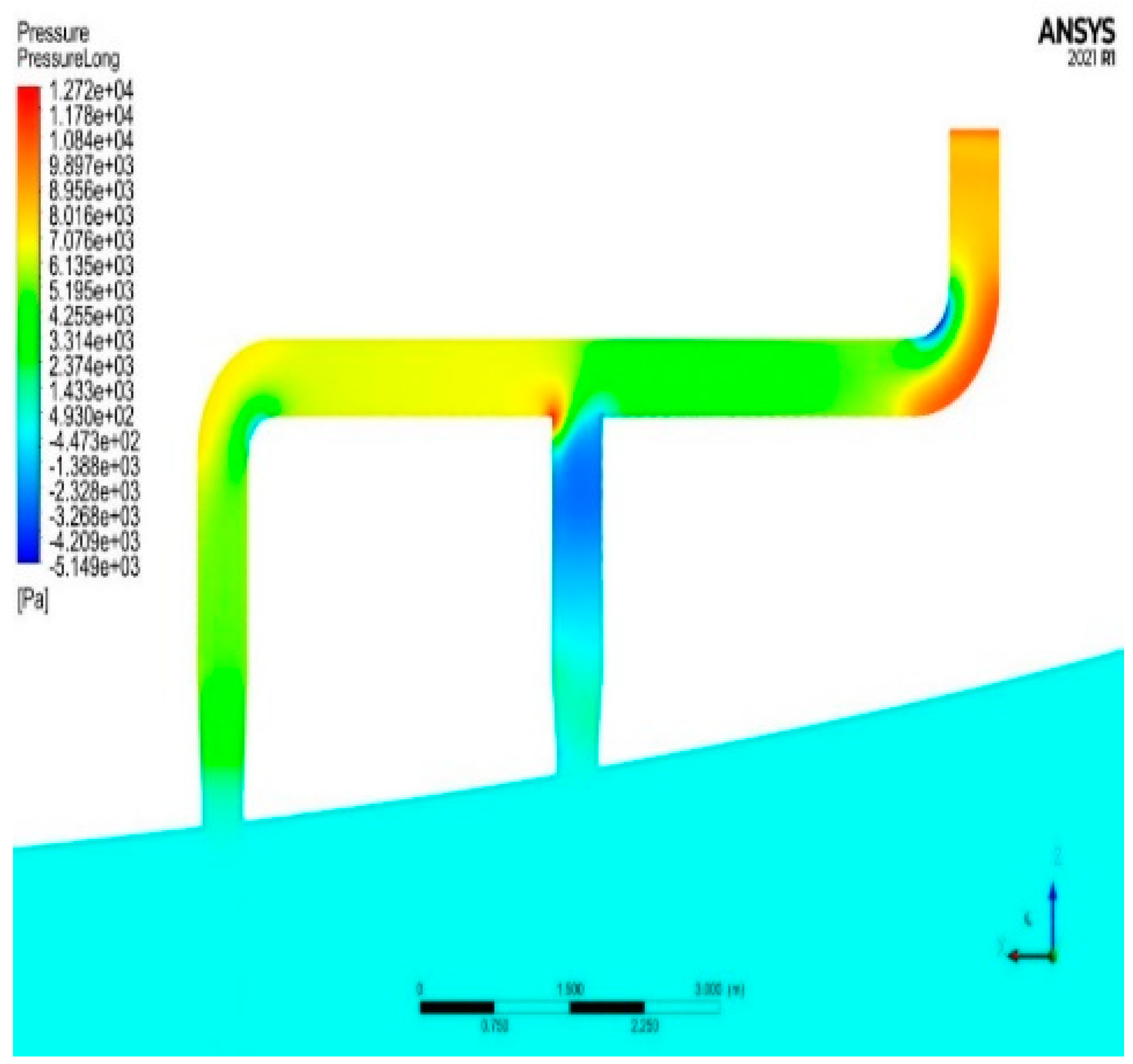
2.3. Domain Boundaries

Based on Figure 3, the boundaries used are [18,19]:

−

opening, for the water volume situated on the fore and aft side of the ship, for the outer water domain facing from ship shell and to the water surface, and also under the keel area; this boundary condition allows the fluid to cross the boundary surface in either direction. For example, all of the fluid might flow into the domain at the opening, or all of the fluid might flow out of the domain, or a mixture of the two might occur.

−

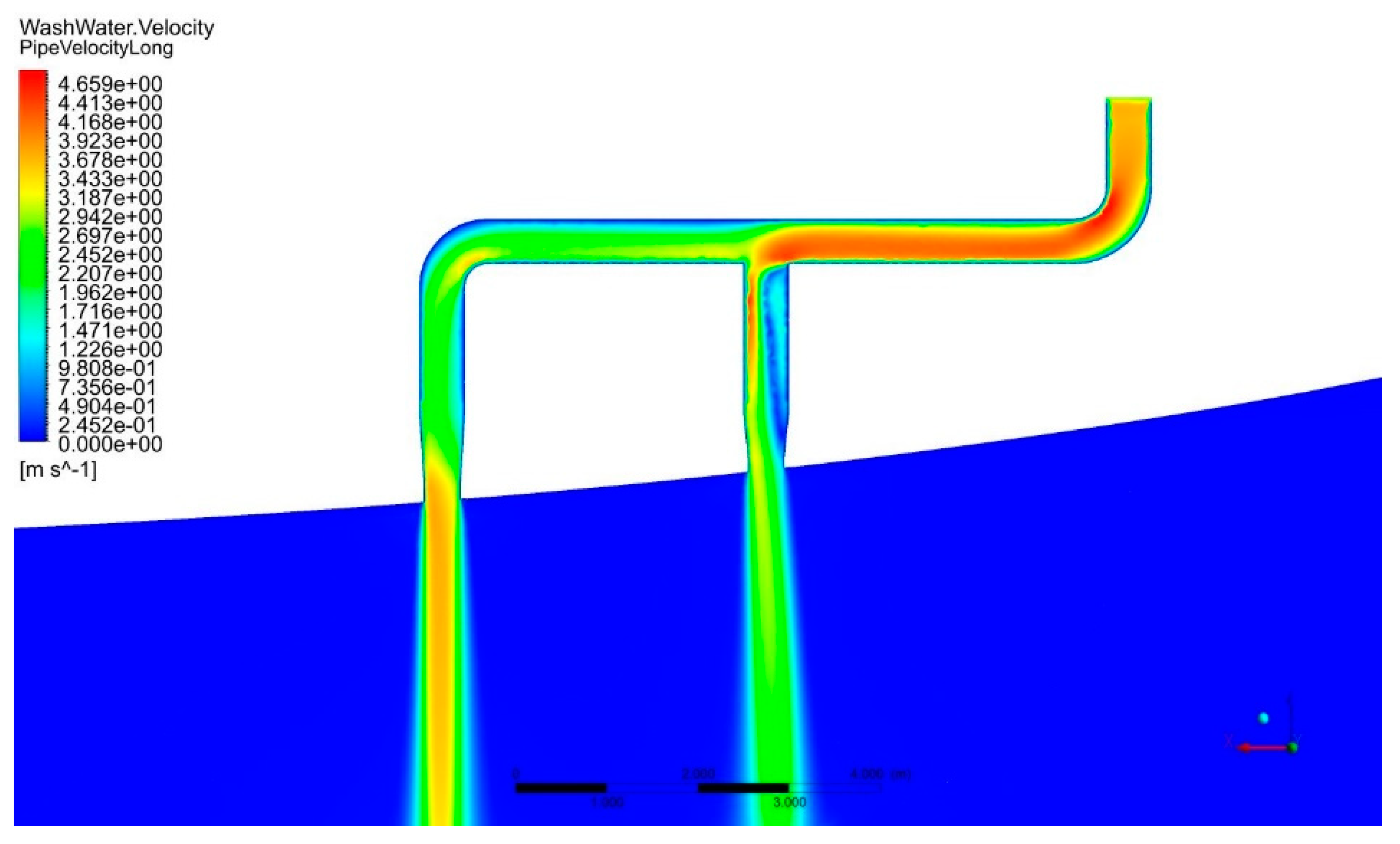
inlet, only for the pipe surface situated before the two openings in the side shell; for the subsonic inlet, the magnitude of the inlet velocity is specified, and the direction is taken to be normal to the boundary. The direction constraint requires that the flow direction, D_i, is parallel to the boundary surface normal, which is calculated at each element face on the inlet boundary.

The boundary velocity components are specified, with a non-zero resultant into the domain.

$$U_{inlet}=U_{spec}i+V_{spec}j+W_{spec}k$$

(1)

The mass flow rate, defined within the simulation, is considered to be uniform and normal to the boundary. The mass influx [20] will be calculated by using:

$$\rho U=\frac{\dot{m}}{\iint dA}$$

(2)

where $\iint dA$ is the integrated boundary surface area at a given mesh resolution.

−

wall, for the ship shell and pipe walls; there was considered a No Slip wall, with the velocity of the fluid at the wall boundary of 0.

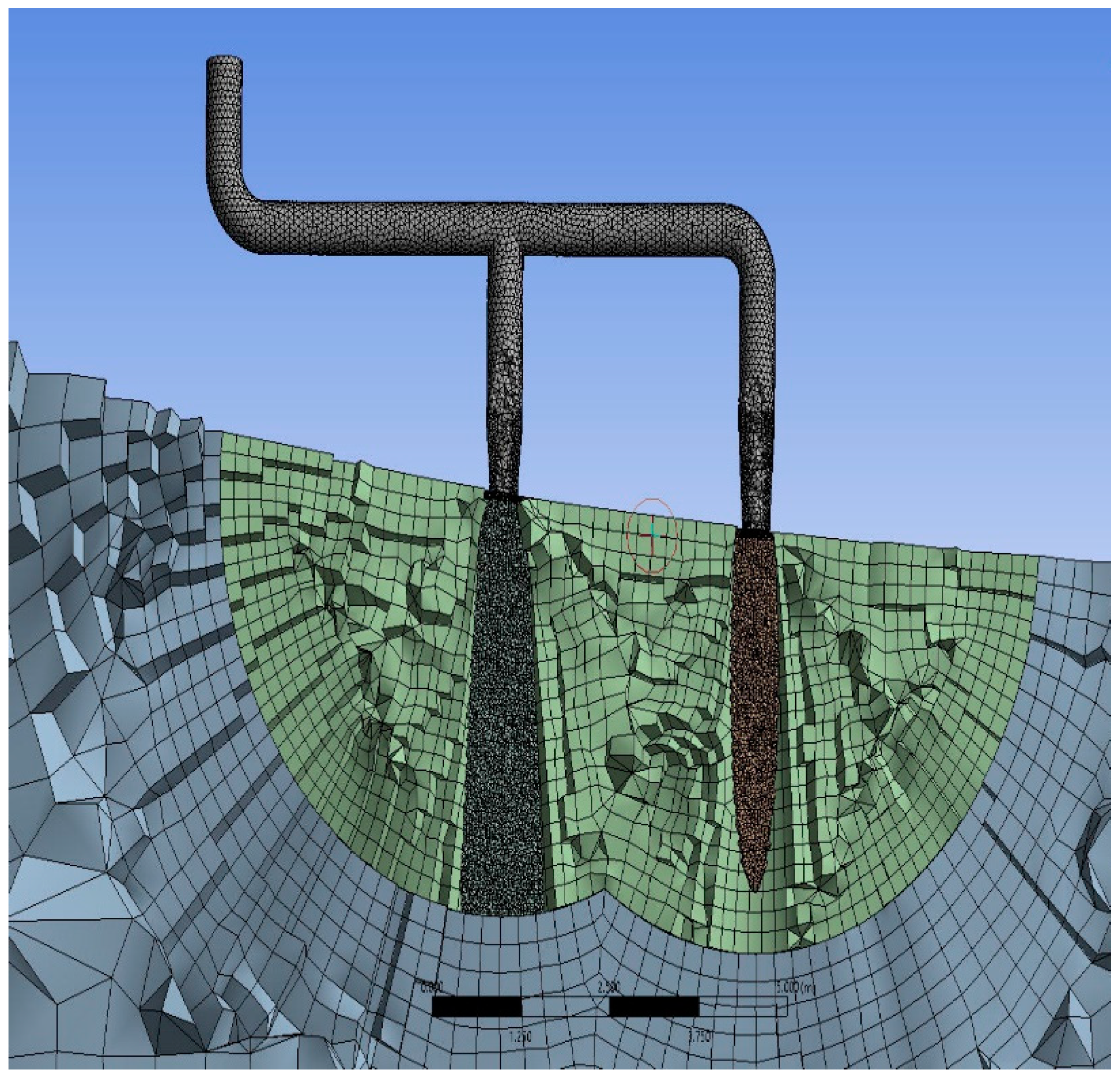
2.4. Mesh Details

In order to achieve appropriate results, a structured mesh was used based on the hex-dominant method. Within the ship shell volume of influence, the maximum length for elements was considered to be 0.3 m for all points at a 4 m distance from the center of the spherical volumes. In the center of the spherical volumes, we designed a mesh based on refinement cones using a maximum element length of 0.04 m. This is considered to be the main area of interest and the decision for these local refinements is made for simulation accuracy. The described mesh with refinement cones is presented in Figure 4. The metrics for the current mesh are presented in

Table 1. Data for the considered mesh with refinement cones.

Domain	Nodes	Elements	Tetrahedra	Hexaedra
D 400 LC	1684594	925743	774419	129569

. The selected mesh for 3D scrubber wash water discharge pH modelling has near 1 million elements, contributing to a precise result and a faster computational process for the identified initial conditions.

3. Simulation Model Description

3.1. Turbulence Model

The flow within the computational domain is a fully turbulent flow and, given the simulation objectives, the near-wall flow prediction is not necessary. Based on these assumptions, the standard k–ε; turbulence model was used. The model is a semi-empirical one [20,21]; the rate of dissipation (ε) and turbulence kinetic energy (k) are based on the below transport equations [20]:

$$\frac{\partial }{\partial t}\left(\rho k\right)+\frac{\partial }{\partial x_i}\left(\rho k{u}_i\right)=\frac{\partial }{\partial x_j}\left[\left(\mu +\frac{\mu }{{\sigma }_k}\right)\frac{\partial k}{\partial x_j}\right]+G_k+G_b-\rho \epsilon -Y_M+S_k$$

(3)

$$\frac{\partial }{\partial t}\left(\rho \epsilon \right)+\frac{\partial }{\partial x_i}\left(\rho \epsilon u_i\right)=\frac{\partial }{\partial x_j}\left[\left(\mu +\frac{\mu }{{\sigma }_{\epsilon }}\right)\frac{\partial \epsilon }{\partial x_j}\right]+C_{1\epsilon }\frac{\epsilon }{k}\left(G_k+C_{3\epsilon }{G}_b\right)+C_{2\epsilon }\frac{{\epsilon }^2}{k}+S_{\epsilon }$$

(4)

where G_k represents the generation of turbulence kinetic energy due to the mean velocity gradients, G_b is the generation of turbulence kinetic energy due to buoyancy, Y_M represents the contribution of the fluctuating dilatation in compressible turbulence to the overall dissipation rate, C_1ε, C_2ε, and C_3ε are constants, σ_k and σ_ε are the turbulent Prandtl numbers for k and ε, while S_k and S_ε are user-defined terms.

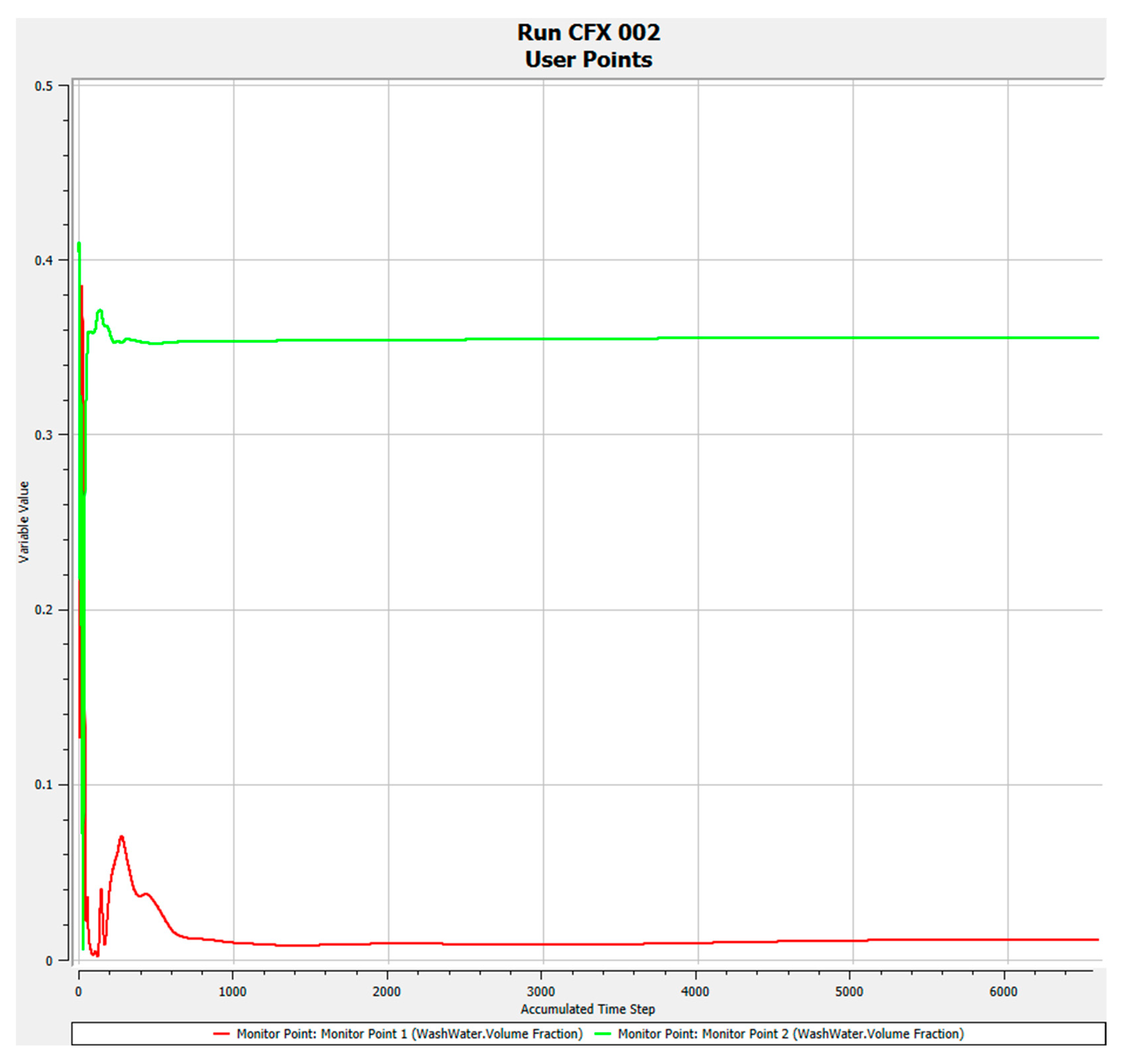
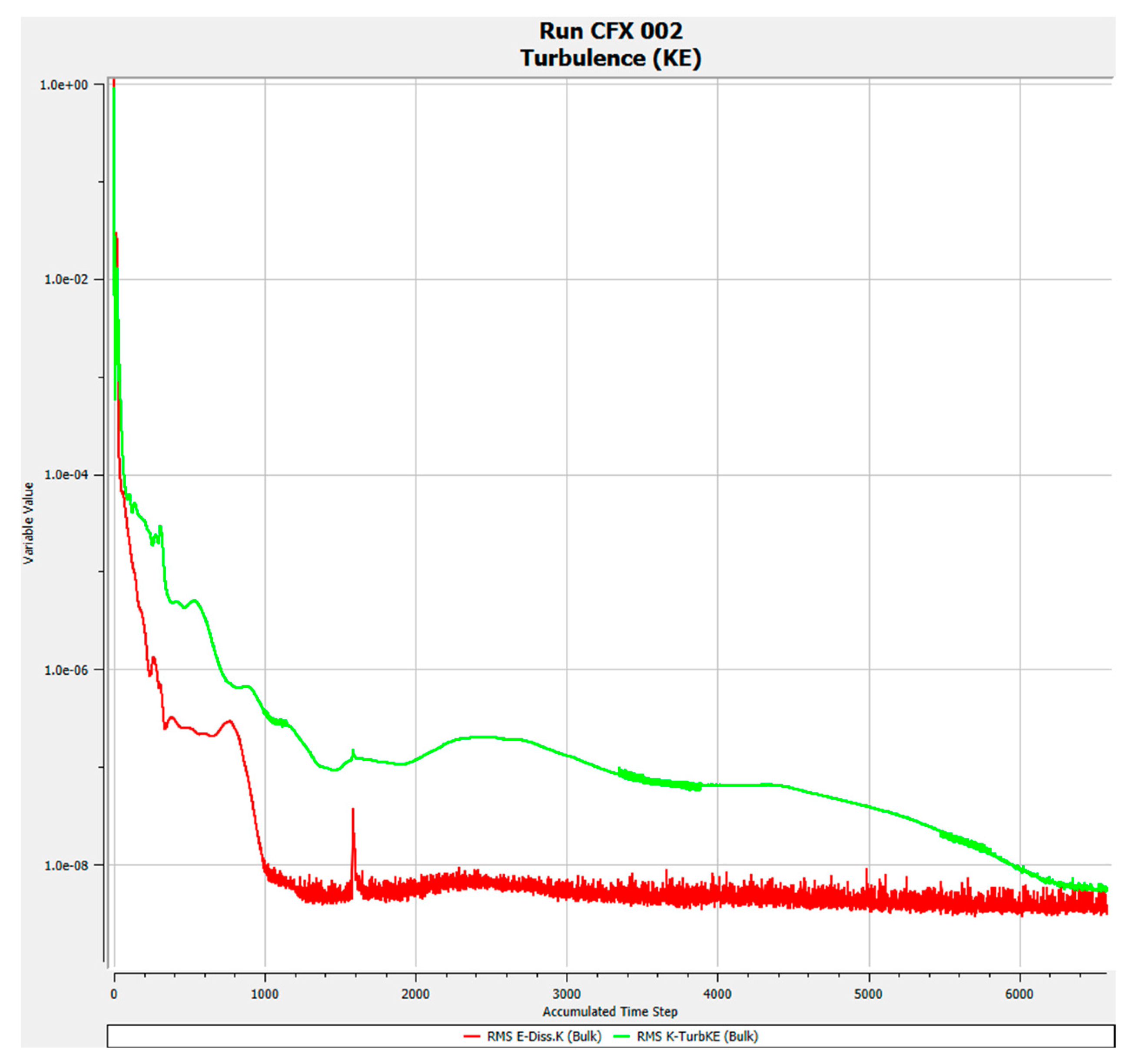
3.2. Simulation Sensitivity and Stability

In order to identify a proper way to investigate the scrubber wash water dilution process, we will consider two factors that are affecting the simulation in a 3D computational domain: the mesh sensitivity and the solution stability. To assess the mesh influence in the current simulation, three different cases are considered: the initial mesh, the rougher mesh, and the refined mesh. For each case, the mesh metrics are presented in

Table 2. Mesh metrics for the initial mesh, the rougher mesh, and the refined mesh.

Mesh Case	Max Element Length throughout Domain	Probe Volume	Max Element Length in the Interest Area	Nodes	Elements
Initial mesh	0.7 m	0.3 m	0.04 m	1684594	925743
Rougher mesh	0.7 m	0.3 m	0.06 m	1223629	620681
Refined mesh	0.7 m	0.18 m	0.03 m	2072666	1188839

. The variation of maximum element length in the area of interest (0.08 m, 0.04 m, and 0.03 m). The results are presented in Figure 5, Figure 6 and Figure 7.

For all considered mesh developments, the solution was considered to be converging after the first 1000 iterations, and the residual values development within the carried iterations was clearly stable. The results for scrubber wash water pH modelling are stable and present similar shape; the obtained results values are not highly dependent on the mesh refinement level.

For a better comparison and understanding of the simulation results, we used the peak volume fraction results for the area of interest (4 m radius probe sphere). The values obtained in the presented cases are shown in

Table 3. Peak volume fraction for each case.

Mesh Case	Peak Volume Fraction
Initial mesh	0.4013
Rougher mesh	0.3895
Refined mesh	0.4086

. The achieved differences are small, established in a range of max 3% variation, related to the initial mesh setting, which leads to the conclusion that the solution is stable and can also be considered acceptable.

The results from the variation of maximum element length in the area of interest (0.08 m, 0.04 m, and 0.03 m) bring us to the conclusion that the initial used mesh meets the required conditions for consistency and stability of the results based on the stability of the results and on the convergence trend and achievement. The results are less sensitive to mesh metrics in the range presented, and each case can be a way to investigate the optimal results for further analytical research. Due to this conclusion and the lower number of elements, the initial setup will be used in the 3D scrubber wash water dilution study.

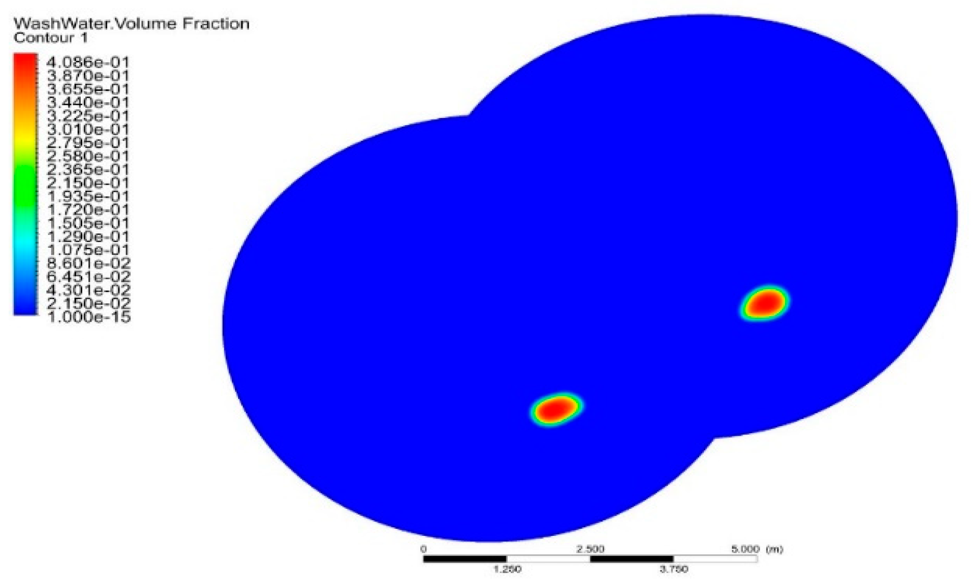
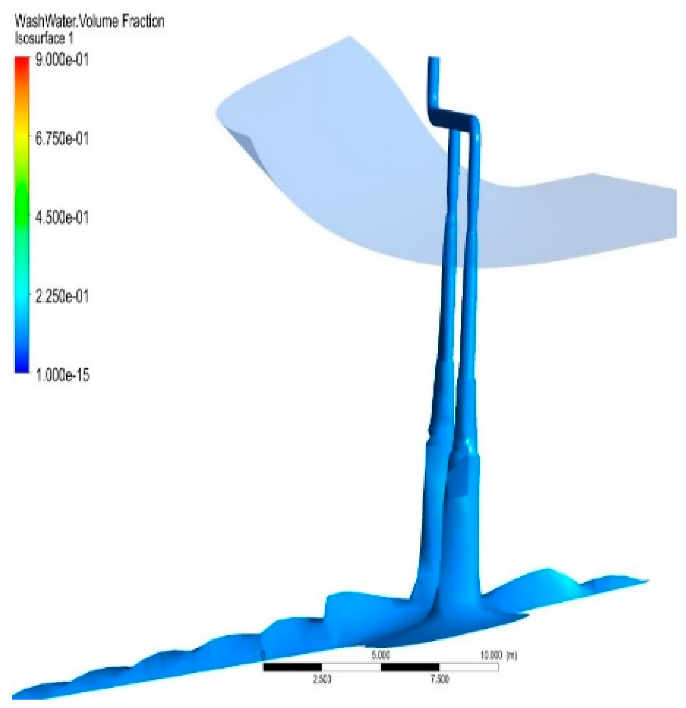
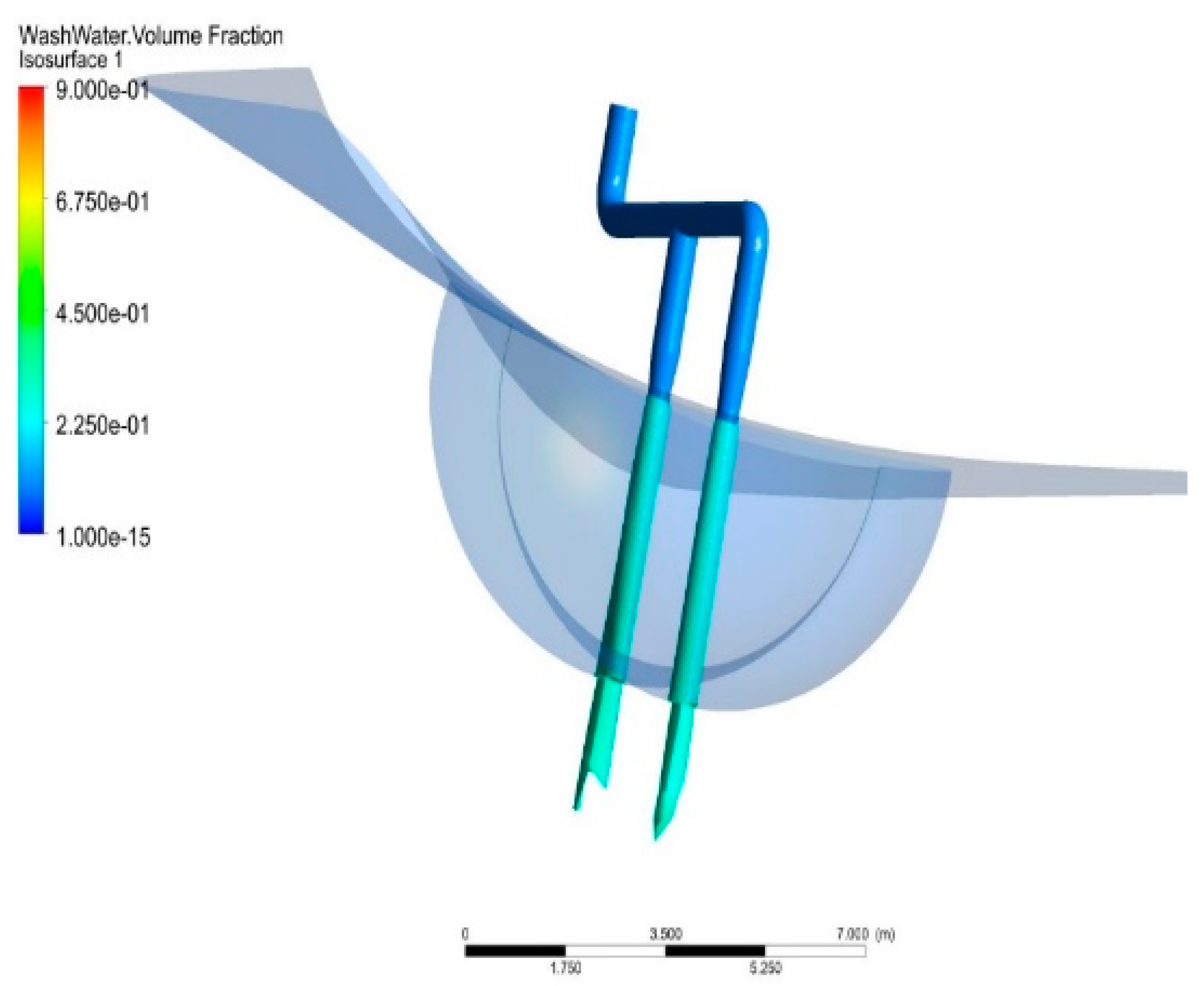
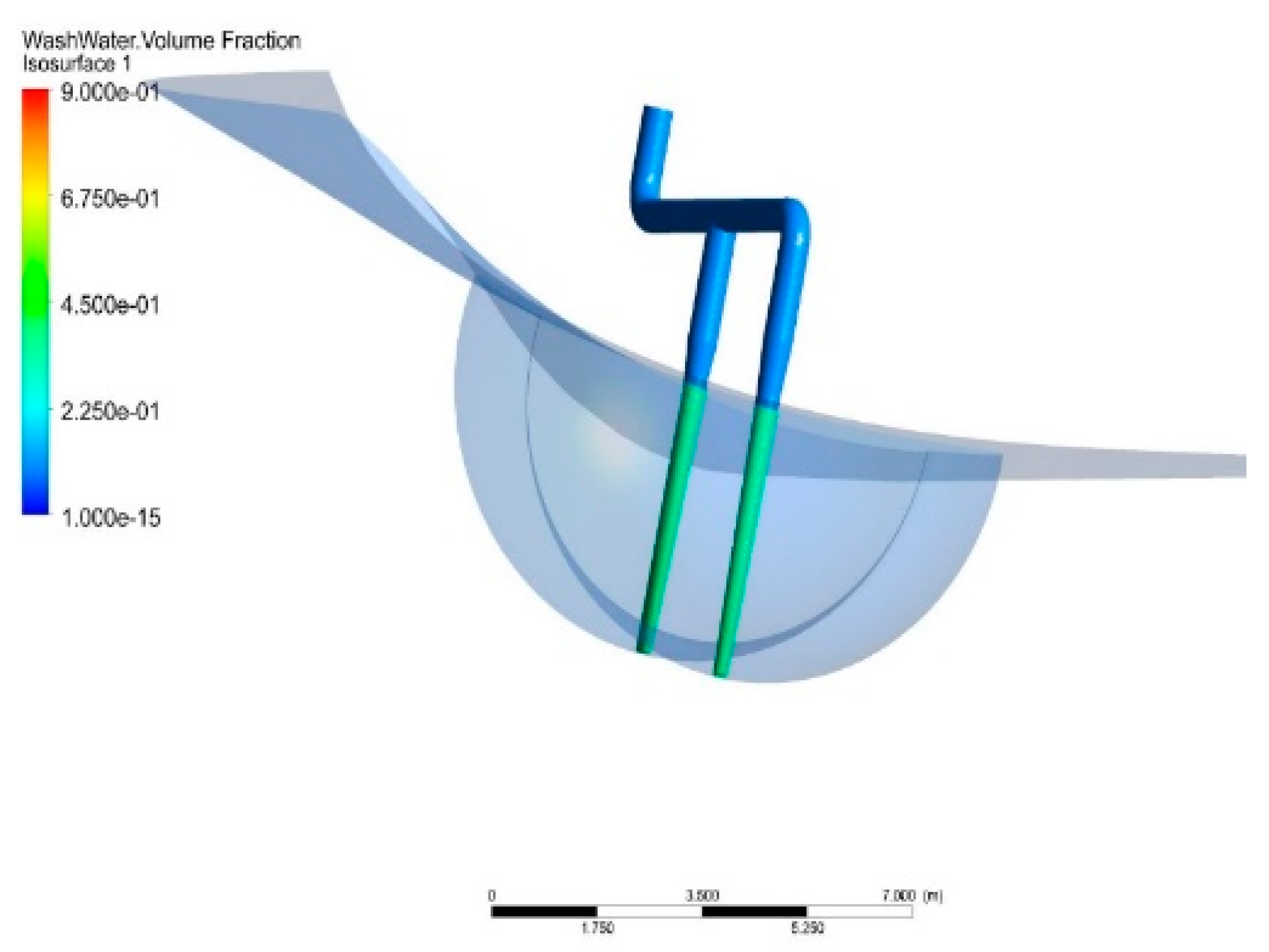
3.3. Scrubber Wash Water pH Development Study

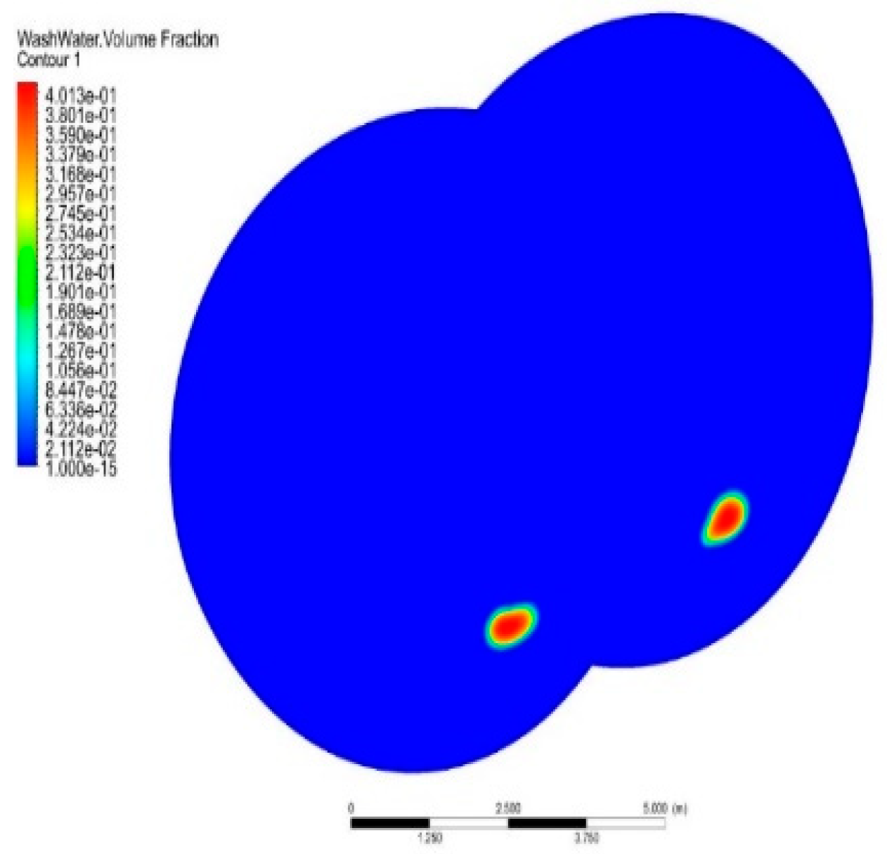
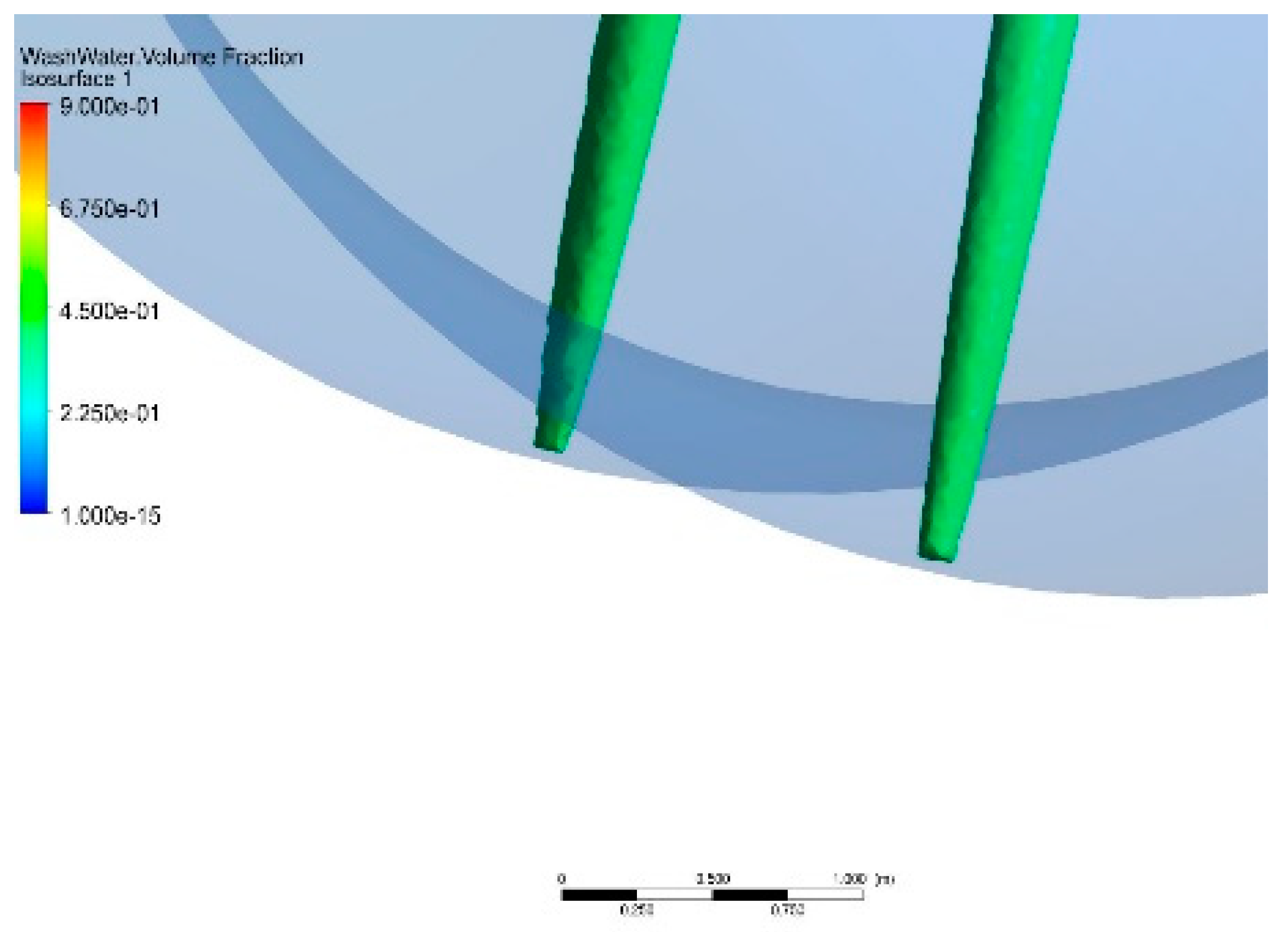
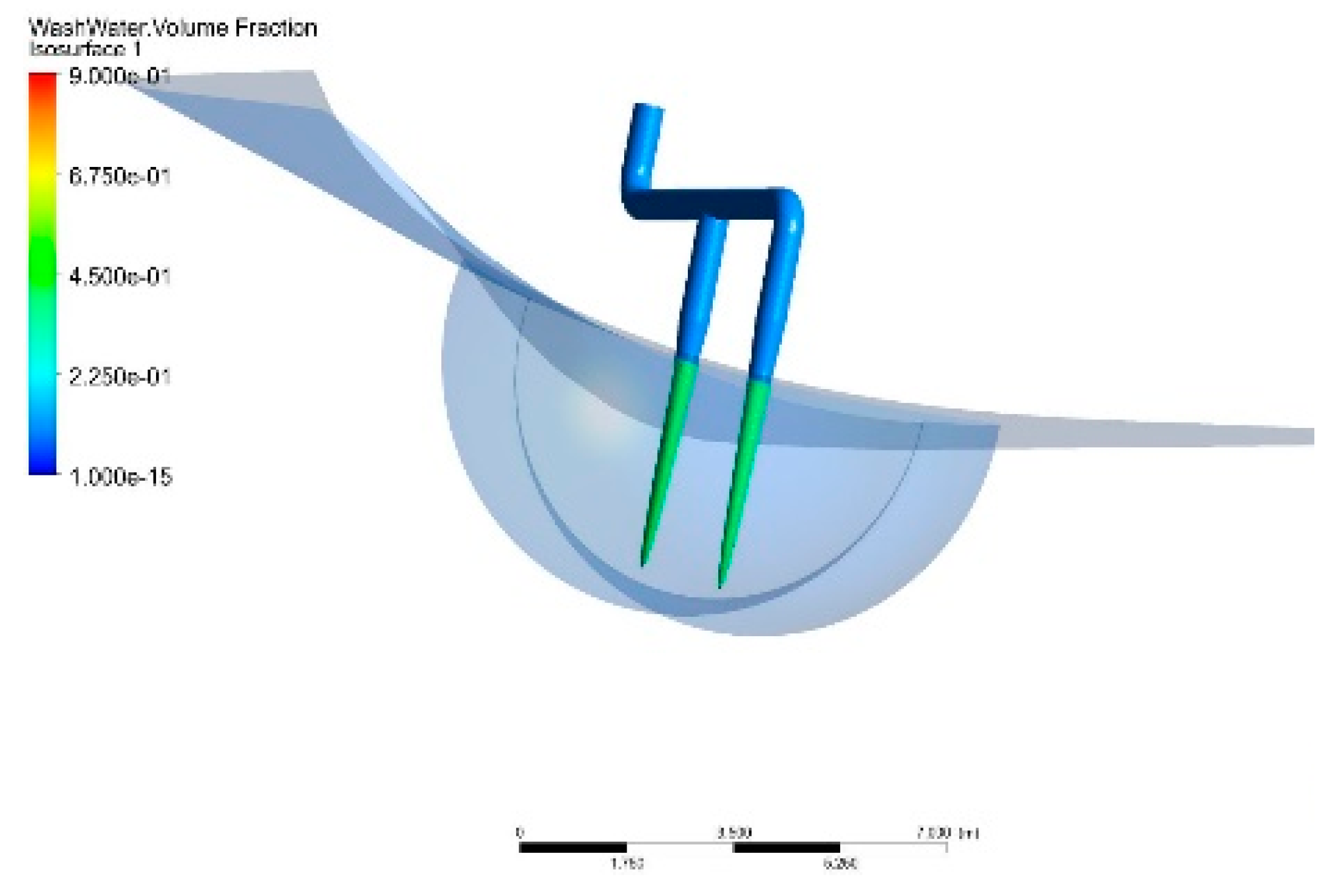
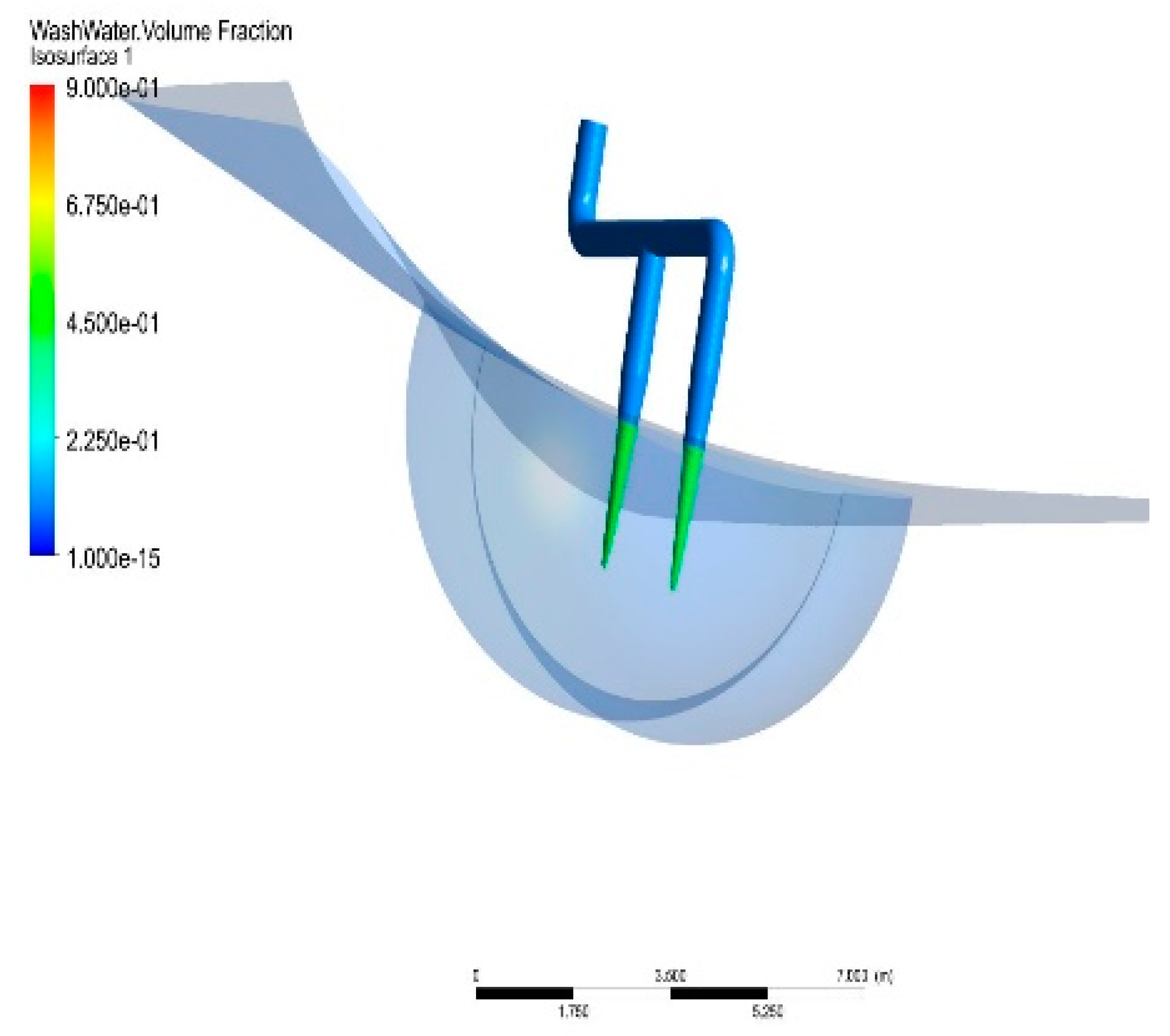
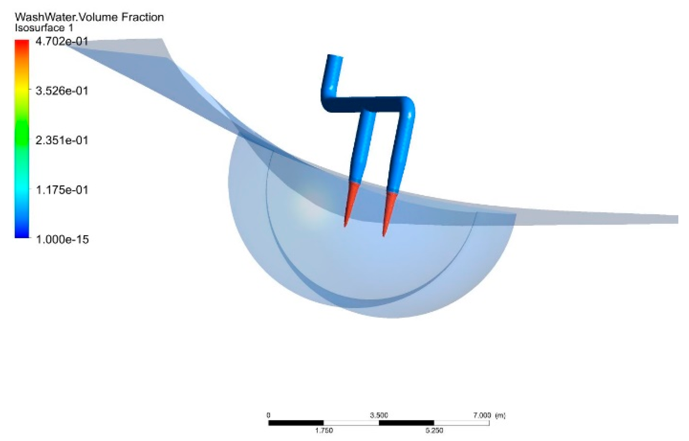
The usage of the initial mesh, with a 400 mm hydraulic diameter for the two outlets, as stated in the initial setup, represents a difficult computational task. Results in the simulation run should meet the stability and convergence criteria. The convergence criteria for the residuals value were set at 10⁻⁹ and required 6500 iterations to obtain a solution.

The considered load case was developed using a 400 mm hydraulic diameter outlet and uses the highest operational value of the wash water flow (3050 m³/h), according to MEPC.259(68) and IMO’s PPR 2/2/3. This evaluates the dilution ratio at a distance of 4 m from the hull in any direction during stationary operation. Data for this load case are presented in

Table 4. Load case parameters.

Ship Speed [kn]	ME Load [%]	Power Plant Load [%]	Wash Water Flow [m3/h]	Wash Water Mass Flow [kg/s]	Wash Water Velocity [m/s]	Hydraulic Diameter [mm]
0	85	75	2600 + 450	868.4	4.31	400

.

4. Results

The simulation results for velocity, pressure, and wash water volume fraction are presented in Figure 8, Figure 9, Figure 10, Figure 11, Figure 12, Figure 13, Figure 14, Figure 15, Figure 16, Figure 17, Figure 18, Figure 19 and Figure 20. During the post-processing process, we use isosurfaces to show the results at the MEPC’s required distance from the outlet.

In Figure 10, Figure 11 and Figure 12, the pressure and velocity values in the longitudinal and transversal sections of the pipe are shown, and they can be considered as an additional check regarding the validity of the computational setup, taking into account the discharge water flow rate of 3050 m³/h and the pipe outlet hydraulic diameter. Figure 13, Figure 14, Figure 15, Figure 16, Figure 17, Figure 18, Figure 19, Figure 20, Figure 21 and Figure 22 show the isosurface representations for relevant scrubber wash water volume fractions.

5. Discussion

As stated within the introductory section of this article, based on the existing rules and regulations [13,16,17] and taking into account the available findings in the theoretical and practical studies and results [4,12], the maximum acceptable volume fraction of the scrubber wash water flow, at 4 m distance from the outlets, is deemed to be 0.47, for which the pH value of the diluted wash water is a minimum of 6.5.

Based on the initial mesh for the geometry used, specific results were obtained and can be considered as a starting point for further discussions and studies regarding the optimal values for the scrubber wash water dilution process and related requirements. A comparative analysis based on the obtained results is made in terms of dilution for the considered load case.

The numerical results presented for the scrubber wash water pipes in terms of velocity (Figure 10 and Figure 11) and pressure (Figure 12) highlight the flow parameters, taking into account the possible vibrations that can appear at both pipe level and hull opening connection. The higher the velocity, the higher the vibration level, especially for strainers, valves, and elbows.

The flow modelling results contains basic information for ship wash water investigated according to applicable international standards, in compliance with MEPC 259(68).

During operation of the scrubber, wash water is fed from two hull openings (corresponding with the wash water outlet) and the result is a turbulent jet behavior that can be visualized and processed via the simulation results as a scalar scale or isosurface. The most relevant isosurface shown in the results is the one based on Volume Fraction (VF) because the scrubber wash water and seawater are modelled as Volume Fraction models.

As a measure of quality check, we use unity check, and the resulting value is 0.853, which confirms the results within the acceptable results parameter range. The wash water concentrations obtained were checked against the acceptable values and centralized in

Table 5. The centralized values for wash water dilution.

Model Particulars	Maximum Volume Fraction	Acceptable Volume Fraction	Unity Check
400 mm hydraulic diameter	0.4013	0.47	0.853

.

Based on the results obtained, it can be observed (Figure 17, Figure 18 and Figure 19) that the maximum Volume Fraction value for the scrubber wash water is 0.4013 on the 4 m radius control sphere. A unity check value of 0.85 can be observed, which is deemed to be within acceptable limits (by considering a conservative approach). The main interest for the flow development is the dilution ratio achieved against the required value in order to meet the approval and certification criteria.

The present simulation can be considered as developed based on an ultraconservative approach, obtained in this case by the applied simplifications, e.g., the removal of the turbulence enhancing appendages and using a No Slip wall, without any material roughness, as boundaries, but also taking into consideration the real operational situation, which is further developed in the paragraph below.

The MEPC rule, as interpreted both in the subsequent guidelines and also in the simulation setup, requires two totally opposite operational conditions to be met: on the one hand, the flow around the ship hull is null, therefore, the ship is considered to be static, without any current in the area; on the other hand, the load of the scrubber system must be considered as the nominal load, which corresponds to an ME load of a minimum of 85%, a power plant load of a minimum of 75% (see Table 4), and the nominal wash water flow of 3500 m³/h. This particular situation will never be found in real life; therefore, we can easily consider that the operational situation for a static ship is closer with a 75% load of the power plant and 0% load for ME, resulting in a substantially decreased exhaust gas flow, “washed” with the nominal scrubber wash water flow, of 3500 m³/h. The natural assumption, based on these facts, is that the real initial value of the scrubber wash water pH at the ship’s openings will be higher than the value already considered within the simulation setup (of 3), and in such a situation, the minimum acceptable wash water Volume Fraction values are, in a real operational situation, more relaxed than the ones used in the present approach.

6. Conclusions

The 3D model and the computational domain used for developing the scrubber wash water dilution modelling are adopted based on a real ship hull design, taking into consideration the existing IMO rules which are regulating the process.

The increased number of retrofitting projects aiming to decrease the exhaust gas emissions SO_x content in the shipbuilding industry through the use of exhaust gas scrubbers comes with various side challenges, such as preserving the overall water quality during the scrubber operation and not affecting the water pH (or achieving the smallest possible impact). These requirements are enforced by international bodies such as IMO (International Maritime Organization) via MEPC resolutions, and they are monitored or certified by Class Registers. Based on the aforementioned situation, the requirements for carrying out specific dilution studies through the use of CFD analysis are, sometimes, generating a need for determining good practice in carrying out the simulations, and also for creating a benchmarking database for the simulation approach, technical solution pursued, and the results obtained.

The existing results and simulation setup, corroborated with the real operational situation, leads to a possible conclusion that the actual rules and their interpretation are forcing an ultraconservative way of developing the related studies and the calculation of the allowable values in the area of interest. Nevertheless, a database with experimental results in the 4 m distance range, together with the functional parameters of the system in various cases are required to defend this affirmation and can represent future research related to this topic.

Future scrubber wash water research will be directed both to the simulation using various flows and velocities for the washwater, and also regarding the possible influence of acidic water on other inlets from other systems which are placed in the vicinity of the scrubber wash water outlet.

References

1. Atkins, P.W.; De Paula, J. Physical Chemistry; Oxford University Press: Oxford, UK, 2006. [Google Scholar]
2. Batchelor, G.K. An Introduction to FLUID Dynamics; Cambridge University Press: Cambridge, UK, 2001. [Google Scholar]
3. Bronsted, J.N. Some remarks on the concept of acids and bases. Recl. Trav. Chim. Des Pays-Bas 1923, 42, 718–728. Available online: https://www.chemteam.info/Chem-History/Bronsted-Article.html (accessed on 6 January 2022).
4. Choi, Y.S.; Lim, T.W. Numerical Simulation and Validation in Scrubber Wash Water Discharge from Ships. J. Mar. Sci. Eng. 2020, 8, 272. [Google Scholar] [CrossRef] [Green Version]
5. Renforth, P.; Henderson, G. Assessing Ocean alkalinity for carbon sequestration. Rev. Geophys. 2017, 55, 636–674. [Google Scholar] [CrossRef]
6. Flagiello, D.; Esposito, M.; Di Natale, F.; Salo, K. A Novel Approach to Reduce the Environmental Footprint of Maritime Shipping. J. Marine. Sci. Appl. 2021, 20, 229–247. [Google Scholar] [CrossRef]
7. Qureshi, M.A.A.; Tahir, R.M. The Implementation of Water Salinity Tester as a quantitative tool to determine the Total Dissolved Solids in water. Tech. Rom. J. Appl. Sci. Technol. 2021, 3, 1–8. [Google Scholar]
8. Available online: www.valmet.com (accessed on 28 March 2021).
9. Teuchies, J.; Cox, T.J.S.; Van Itterbeeck, K.; Meysman, F.J.; Blust, R. The impact of scrubber discharge on the water quality in estuaries and ports. Environ. Sci. Eur. 2020, 32, 103. [Google Scholar] [CrossRef]
10. Khan, Z.H. Relation Among Temperature, Salinity, pH and DO of Seawater Quality. Tech. Rom. J. Appl. Sci. Techn. 2020, 2, 39–45. [Google Scholar] [CrossRef]
11. Brown, K.; Kalata, W.; Schick, R. Optimization of SO2 Scrubber using CFD Modelling. In Proceedings of the “SYMPHOS 2013”, 2nd International Symposium on Innovation and Technology in the Phosphate Industry, Agadir, Morocco, 6–10 May 2013. [Google Scholar]
12. Ulpre, H. Turbulent Acidic Discharges into Seawater. Ph.D. Thesis, University College London, London, UK, 2015. [Google Scholar]
13. Marine Environment Protection Committee. Resolution MEPC.259 (68)—Guidelines for Exhaust Gas Cleaning Systems; Marine Environment Protection Committee: London, UK, 2015. [Google Scholar]
14. Bureau Veritas—Rules for the Classification of Steel Ships—PART C and PART F—Machinery, Electricity, Automation and Fire Protection. Available online: https://marine-offshore.bureauveritas.com/nr467-rules-classification-steel-ships (accessed on 6 January 2022).
15. DNV-GL. Rules for Classification, Part 4—Systems and Components; DNV-GL: Høvik, Norway, 2018. [Google Scholar]
16. DNV-GL. pH Discharge Criteria for Exhaust Gas Cleaning Systems according to MEPC.259(68); DNV-GL: Høvik, Norway, 2015. [Google Scholar]
17. International Maritime Organization—Sub-committee on Pollution Prevention and Response (PPR 2/2/3). Application of Calculation-Based Methodology for Verification of the Washwater Discharge Criteria for pH in Section 10.1.2.1(ii) of the 2009 Guidelines for Exhaust Gas Cleaning Systems. Available online: https://edocs.imo.org/Processing/English/PPR (accessed on 13 November 2014).
18. Ansys Inc. Ansys CFX Solver Theory Guide. Ansys CFX Release 2009, 15317, 724–746. [Google Scholar]
19. Stachnik, M.; Jakubowski, M. Multiphase model of flow and separation phases in a whirlpool: Advanced simulation and phenomena visualization approach. J. Food Eng. 2020, 274, 109846. [Google Scholar] [CrossRef]
20. Le, T.C.; Hong, G.H.; Lin, G.Y.; Li, Z.; Pui, D.Y.; Liou, Y.L.; Wang, B.-S.; Tsai, C.-J. Honeycomb wet scrubber for acidic gas control: Modelling and long-term test results. Sustain. Environ. Res. 2021, 31, 21. [Google Scholar] [CrossRef]
21. Dendy Adanta, I.M.; Rizwanul, F.; Nura Muaz, M. Comparison of standard k-ε and SST k-ω turbulence model for breastshot waterwheel simulation. J. Mech. Sci. Eng. 2020, 7, 39–44. [Google Scholar] [CrossRef]
Figure 1. Spherical volumes in CFD simulation.
Energies 15 05140 g001
Figure 2. Shell penetration plan for scrubber outlet.
Energies 15 05140 g002
Figure 3. Boundaries of the computational domain.
Energies 15 05140 g003
Figure 4. Computational domain mesh with refinement cones.
Energies 15 05140 g004
Figure 5. Maximum Volume Fraction values for the Scrubber Wash Water (initial mesh).
Energies 15 05140 g005
Figure 6. Maximum Volume Fraction values for the Scrubber Wash Water (rough mesh).
Energies 15 05140 g006
Figure 7. Maximum Volume Fraction values for the Scrubber Wash Water (refined mesh).
Energies 15 05140 g007
Figure 8. Volume fraction plot for convergence check (initial mesh).
Energies 15 05140 g008
Figure 9. RMS residuals for k and ε values (initial mesh).
Energies 15 05140 g009
Figure 10. Velocity variation—pipe longitudinal section.
Energies 15 05140 g010
Figure 11. Velocity variation—pipe transversal section.
Energies 15 05140 g011
Figure 12. Pressure variation—pipe longitudinal section.
Energies 15 05140 g012
Figure 13. Scrubber Wash Water Volume Fraction of 0.1 isosurface development.
Energies 15 05140 g013
Figure 14. Scrubber Wash Water Volume Fraction of 0.2 isosurface development.
Energies 15 05140 g014
Figure 15. Scrubber Wash Water Volume Fraction of 0.3 isosurface development.
Energies 15 05140 g015
Figure 16. Scrubber Wash Water Volume Fraction of 0.4 isosurface development.
Energies 15 05140 g016
Figure 17. Scrubber Wash Water Volume Fraction of 0.41 isosurface development.
Energies 15 05140 g017
Figure 18. Scrubber Wash Water Volume Fraction of 0.41 isosurface development—probe sphere detail.
Energies 15 05140 g018
Figure 19. Scrubber Wash Water Volume Fraction of 0.42 isosurface development.
Energies 15 05140 g019
Figure 20. Scrubber Wash Water Volume Fraction of 0.43 isosurface development.
Energies 15 05140 g020
Figure 21. Scrubber Wash Water Volume Fraction of 0.44 isosurface development.
Energies 15 05140 g021
Figure 22. Scrubber Wash Water Volume Fraction of 0.45 isosurface development.
Energies 15 05140 g022