Forecasting of Power Quality Parameters Based on Meteorological Data in Small-Scale Household Off-Grid Systems

Abstract

Off-grid power systems are often used to supply electricity to remote households, cottages, or small industries, comprising small renewable energy systems, typically a photovoltaic plant whose energy supply is stochastic in nature, without electricity distributions. This approach is economically viable and conforms to the requirements of the European Green Deal and the Fit for 55 package. Furthermore, these systems are associated with a lower short circuit power as compared with distribution grid traditional power plants. The power quality parameters (PQPs) of such small-scale off-grid systems are largely determined by the inverter’s ability to handle the impact of a device; however, this makes it difficult to accurately forecast the PQPs. To address this issue, this work compared prediction models for the PQPs as a function of the meteorological conditions regarding the off-grid systems for small-scale households in Central Europe. To this end, seven models—the artificial neural network (ANN), linear regression (LR), interaction linear regression (ILR), quadratic linear regression (QLR), pure quadratic linear regression (PQLR), the bagging decision tree (DT), and the boosting DT—were considered for forecasting four PQPs: frequency, the amplitude of the voltage, total harmonic distortion of the voltage ($TH{D}_u$), and current ($TH{D}_i$). The computation times of these forecasting models and their accuracies were also compared. Each forecasting model was used to forecast the PQPs for three sunny days in August. As a result of the study, the most accurate methods for forecasting are DTs. The ANN requires the longest computational time, and conversely, the LR takes the shortest computational time. Notably, this work aimed to predict poor PQPs that could cause all the equipment in off-grid systems to respond in advance to disturbances. This study is expected to be beneficial for the off-grid systems of small households and the substations included in existing smart grids.

1. Introduction

Electricity is one of the basic necessities of life; it is needed to power homes, factories, and even entire cities. Given that the fuel used in traditional power plants for electricity generation contributes toward environmental pollution, modern power plants employ renewable energy to generate electricity. The use of renewable energy sources has been widely promoted because it helps reduce the carbon footprint [1]. Consequently, the construction of modern power plants has increased considerably, and such power plants are either operated separately (i.e., off-grid systems) or connected to an external power grid (i.e., on-grid systems). Currently, power grids require smart systems for their operation. However, it remains challenging to develop a smart system that is able to both control the power grid production and maintain the generated power within power quality limits as far as possible [2]. Power quality is typically evaluated using power quality parameters (PQPs) according to specific standard ranges [2]. These parameters include harmonics, power frequency variations, voltage and current imbalances, transients, flickers, and voltage sag or dips. Among these, the most important parameters are the magnitude of the supply voltage, power frequency, total harmonic distortion of voltage ($TH{D}_u$), and total harmonic distortion of current ($TH{D}_i$) [2]. Accordingly, this study focuses on these parameters. Although many previous studies have focused on reconfiguring on-grid power systems, few studies have focused on off-grid systems; this is discussed in detail in Section 2. For the development of smart control models, two main aspects should be considered: a forecasting model (the main and most challenging aspect) and an optimisation model [3,4]. The forecasting process is an important part of smart control units; however, applying real-time smart control systems with renewable energy (off-grids) remains challenging and unaddressed, owing to the nonlinearity of weather conditions. To address this issue, this study aimed to test three prediction models with an artificial neural network (ANN), a decision tree (DT), and linear regression (LR) for predicting (PQPs) using power and weather data. The mean absolute percentage error (MAPE) was then used to evaluate and compare the prediction results. In this work, an experimental off-grid platform based on an AC/DC system was employed. This experimental off-grid platform was developed by a team from the ENET Centre, which is located on the campus of VŠB-Technical University of Ostrava. The main purpose of this experimental off-grid platform is to simulate households with common household appliances, thus contributing toward the development of modern green technologies, such as vehicle to grid technology [5,6] or research on prediction and optimisation [7,8,9].

The contributions of this work can be summarised as follows:

• An innovative concept for forecasting the PQPs of household off-grid systems is presented.
• The accuracies of forecasting models based on PQP datasets with meteorological data are compared considering household off-grid environments.
• The computation times of these forecasting models are also compared.

The remainder of this paper is organised as follows. Section 2 provides a literature review of the related works. Section 3 describes the off-grid hardware, appliances, and data acquisition. Section 4 addresses the theory governing the prediction method used in this study, Section 5 describes the proposed model, Section 6 summarises the results of the experiments, and Section 7 discusses these results. Lastly, Section 8 presents the conclusions drawn based on this study.

2. Related Work

The development of smart power systems, especially off-grid systems, is significantly challenging. This section discusses previous research focusing on the prediction of PQPs, reconfiguration of power systems, and optimisation of power quality, with the overarching goal of generating good-quality power. These previous studies can be divided into two main categories: studies dealing with off-grid systems and studies dealing with on-grid power systems.

2.1. Research on Off-Grid Systems

Among the studies reported in this field, in [10], a random decision forest optimised via multi-objective optimisation was used to predict PQPs (power frequency, amplitude of the voltage, total harmonic distortion, and flicker severity in an off-grid platform). The corresponding simulation results revealed that the forecasting results exceeded 90% for forecasting time step of 15 min. Furthermore, two models, a decision tree and a neural network, have been proposed for the short-term forecasting of five PQPs pertaining to off-grid systems: power frequency, magnitude of the supply voltage, total harmonic distortion of voltage, total harmonic distortion of current, and short-term flicker severity. Based on the experimental results, the proposed approach was evaluated using the average MAPE for six days, and the best results were achieved using the DT [11]. In [12], an ANN with backpropagation was used as learning algorithm for forecasting the following PQPs: power frequency, total harmonic distortion of voltage, total harmonic distortion of current, and long-term flicker severity. This task was used to optimise the power quality of an off-grid system. Moreover, two methods—random forest and extreme learning machines (feedforward neural networks)—were used to forecast the $TH{D}_i$ of the power photovoltaic [13]. A comparison of the results indicated that the prediction performance of the random forest method exceeded that of the neural network. In [14], simple binary classification was used to predict PQPs, focusing on the frequency, $TH{D}_u$, and $TH{D}_i$ forecasting. The performance of the proposed model outperformed that of the system in [12]. Moreover, in [1], ANN was used to forecast the power frequency, $TH{D}_u$, and long-term flicker severity. The model employed referred to weather conditions for the prediction of these PQPs. In [15] proposed model using machine learning and regression techniques for power quality prediction, the model used PQPs values and home appliances as input variables for forecasting PQPs in off-grid system. In [16] a differential polynomial neural network, deep learning, and regression models for predicting PQPs for one day ahead were applied.

2.2. Distribution Power Grid

In [17], a long short-term memory network was used to forecast the voltage and current in a power grid system. This model achieved better results terms of the voltage and current forecasting across the low voltage range, as compared to others. For generating good quality power, [18] proposed the use of machine learning for reconfiguring power systems. This was tested within the IEEE 14-bus and 30-bus systems. The results proved the validity of this suggested approach. To reduce power losses and improve power grid stability, in [19], a genetic algorithm with particle swarm optimisation was employed for power distribution grid reconfiguration. This model used the IEEE 33-bus distribution system. Experimental results confirmed the effectiveness of this system in optimising the power distribution grid. Furthermore, in [20], modified particle swarm optimisation was applied to determine the optimal reconfiguration for a power distribution grid. This system was tested among 33 IEEE bus systems, and the results of the model were compared with those obtained under other modes of the particle swarm optimisation algorithm. Notably, it was concluded that the reduction in power loss could be improved, along with a decrease in the computational time. The optimal configuration of a power distribution grid contributes toward a reduction in the active power losses. In [21], an ANN reduced by modified dynamic fuzzy c-means was used as a model for power system reconfiguration. The proposed model was tested on the IEEE 33-bus and 69-bus systems and also compared with others, it offers the following advantages: simple design, short implementation time, and high efficiency. To reduce active power losses and improve the voltage magnitude, a cuckoo search algorithm was used in [22] to reconfigure a power network. This system was tested for the IEEE 33, IEEE 69, and IEEE 119 distribution systems. Numerical results confirmed the validity of this designed system for power network reconfiguration, as compared with others. Additionally, a grey wolf optimisation algorithm for power network reconfiguration was proposed in [23]. This approach was tested with the standard IEEE 33 bus and IEEE 69 bus distribution networks. Experiments were performed to determine the optimal configuration of the switch combinations combination to achieve the lowest active power loss. Numerical results confirmed confirmed the performance of this designed system. Moreover, real-time autonomous dynamic reconfiguration based on a long short-term memory network for power network restoration [24] was proposed in Taiwan. This approach was tested under two different types of power distribution bus systems. It was concluded that this system requires less computation and can handle unusual cases. In [25], modified selective particle swarm optimisation was proposed to minimise the active losses and optimise the voltage profiles for a power grid system, in order to determine the optimal reconfiguration of the power grid. The model was tested using the IEEE 33-bus system. Experimental results demonstrated that the active power was improved under different load conditions. Manta ray foraging optimisation was applied to achieve the power grid’s optimal restoration. The proposed system was also investigated for the IEEE 33-bus and IEEE 85-bus systems. The performance of the system was compared with that of particle swarm optimisation and grey wolf optimisation. Numerical results showed that the proposed approach was efficient in restoring the power grid [26]. An online network reconfiguration based on a deep q-learning model was also investigated in [27], it was used to determine the best switch combination of the network topology. The performance of this system was compared with that of others, considering two types of power bus systems. Experimental results revealed that this model was more efficient than the others, required less computational time, and applicable for online grid reconfiguration. Binary particle swarm optimisation (BPSO) combined with the traditional particle swarm optimisation (PSO) was developed in [28]. The BPSO algorithm was used to determine the optimal power system restoration, whereas PSO was used to estimate the distributed generation positions. This approach was tested using the IEEE 33-bus and IEEE 69- bus systems, under three different loads. The corresponding results proved the validity of this model in terms of determining the optimal form of switch combination and better locations for distributed generation. Furthermore, a stochastic fractal search (DFS) algorithm was applied to obtain the best switch combination of a power grid. The designed planned pattern was studied with respect to the 33, 69, 84, 119, and 136 bus distribution systems. A comparison of the results showed that the designed framework achieved better solutions than others [29]. To minimise power losses and improve power quality, the Salp swarm algorithm was used to solve the reconfiguration problem for a power grid system. The designed form was studied for different cases with 33-bus and 69-bus distribution system. The corresponding results confirmed the efficiency of this system [30]. Furthermore, other forecast methods are used to optimally design elements or parts of the network [31].

3. Platform Description

The off-grid test platform used for this research simulates the electricity consumption of a typical single-family home. It is an off-grid system based on a hybrid AC/DC architecture. This section provides a detailed overview of this platform.

3.1. Off-Grid Hardware

Figure 1 shows a schematic of the off-grid system used to perform the experiments in this study. This off-grid system consists of two parts: the first part is based on the DC bus, whereas the second part is based on the AC bus. The DC part consists of a Conext XW+ 8548 E hybrid inverter and two Conext 80 600 DC/DC-MPPT solar inverters; these are used to convert photovoltaic (PV) electricity arrays. The off-grid energy storage system uses Hawker 12XFC115 lead-acid batteries connected in parallel. The nominal voltage and capacity of one battery are 12 V and 115 Ah, respectively. These batteries are connected in a battery bank, forming four groups, each including four batteries. The nominal voltage of the main DC bus is 48 V; this voltage varies from 40.5 to 64 V DC depending on the state of charge of the battery and the charging process. The rated power of each of the two PV strings is 2 kW. The solar inverters can supply up to 2 × 80 A to the DC bus. However, the maximum current of each MPPT inverter is limited by the total installed capacity of the PV string and the current battery voltage.

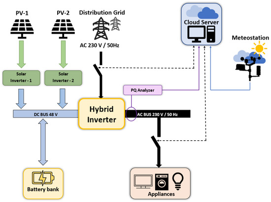
Figure 1. Schematic of off-grid system.

The AC part of the off-grid system is based on a 230 V AC bus with a frequency of 50 Hz. The AC bus is drawn directly from the hybrid inverter to which the individual household appliances are then connected. The primary energy source for the off-grid system is the energy generated by the PV panels. However, considering the atmospheric conditions in Central Europe, it is not economically feasible to meet the off-grid consumption demands using the PV panels and batteries alone. Hence, a conventional distribution energy system was adopted as a second energy source for the off-grid platform [32].

3.2. Off-Grid Appliances

The off-grid test platform includes common appliances, simulating a typical family household.

Table 1 describes the types of appliances, along with the measured electrical values of each appliance. These electrical parameters were measured during the operation of the off-grid power system. Each appliance was measured separately, using a KMB SMC 144 measuring device.

Table 1. Measured electrical characteristics of the appliances used in the experiment [8].

Appliance	Load (W)			Power Actor (-)
	Avg	Min	Max	Avg	Characteristic
Mower	537.6	532.1	549.27	0.52	Inductive
Drill	157.1	149.5	167	0.49	Inductive
Kettle	619.1	617	628.3	1	Resistive
Fridge	207.6	195.5	219.5	0.72	Inductive
AC Heating-AC Cooling	880	852.5	910	0.91	Inductive
Microwave	203	76.8	1348.3	0.84	Inductive
Boiler	307	305.8	346.5	0.99	Inductive
TV	44	42.8	50.5	0.6	Capacitive
Lights	156	152.5	165.1	0.84	Capacitive

3.3. Data Acquisition

3.3.1. Power Quality

The PQ evaluation and measurements were performed in accordance with the European standards EN 50160 and EN 61000-2-2. In our off-grid facility, measurements are performed using the KMB SMC 144 PQ analyser. This analyser measures the power quality across the AC bus and is specially designed for the remote monitoring of energy consumption and its quality. The DIN rail, featuring a display-less design with multiple communication options, is suitable for a wide spectrum of automation tasks associated with modern buildings, infrastructure monitoring, and remote load management. It can monitor parameters such as voltage, currents, flicker, power factors, active power, and reactive power. The measured data are stored in a database for future research on the power optimisation of off-grid systems and PQ prediction. Table 2 shows the individual values of European Standards for PQ.

Table 2. Limits of European Standards for PQPs [2,33].

Parameter	European PQ Standards
	EN 50160	EN 61000-2-2
Voltage frequency	Mean value measured over 10 s ±1% (49.5 Hz–50.5 Hz) for 99.5% of week −6%/+4% (47–52 Hz)  for 100% of week	±2%
Voltage magnitude variations	Mean 10-min RMS values  ±10% for 95% of the week	±10% applied for 15 min
Harmonic Voltage (% of fundamental  supply voltage)	5% 3rd, 6% 5th, 5% 7th, 1.5% 9th, 3.5%, 11th 3% 13th, 0.5% 15th, 2% 17th, 1.5% 19th 23rd and 25th	6% 5th, 5% 7th, 3.5% 11th, 3% 13th, THD <8%

3.3.2. Meteorological Data

The meteorological data used in this study were obtained from a weather station managed by the Czech Hydrometeorological Institute (CHMI); this station is located on the same site as the off-grid building (campus of VSB Technical University of Ostrava). These meteorological data are stored in a database, along with the PQ data, for future comparisons.

4. Formal Methods

4.1. Artificial Neural Network

An ANN is a computational system that attempts to mimic the human brain’s ability to solve certain complex problems. ANNs consist of three main units: the input layer (which accepts the input data and passes them to the hidden layer), the hidden layer(s), and the output layer (which receives the signal from the hidden layer and generates the output signal). A simple ANN consists of one hidden layer, whereas deep learning networks require many hidden layers. Among the many types of ANNs, we used a multilayer ANN with backpropagation as the learning method in this study. The artificial neuron has inputs and a signal output that can be sent to other neurons. All the signal inputs of each neuron are multiplied with an associated weight and summed together as expressed in Equation (1). This summed value is then passed through an activation function to produce the final output of this neuron as indicated in Equation (2). Subsequently, the output of this neuron is passed to the other neurons in the next layer. Many types of activation functions exist, such as the step, linear, and Sigmoid functions. For further details regarding ANNs, please refer to [34].

$$X=\sum _{i=1}^m{x}_i{w}_j$$

(1)

where $x_i$ is the input signal, and $w_j$ is the weight connected between two neuron units

$$output=f\left(X\right)=\left\{\begin{array}{cc}1\hfill & \mathrm{if}\sum x_i{w}_j\ge 0\hfill \\ 0\hfill & \mathrm{if}\sum x_i{w}_j<0\hfill \end{array}\right.$$

(2)

4.2. Multiple Linear Regression

LR serves as a method for establishing a relationship between an input variable (x) and one output signal (y). The output (y) can be estimated based on the combination dataset of the input variables (x) during the learning phase. In the case of one input variable (x), this approach is termed as simple linear regression, as shown in Equation (3). By contrast, in the case of the more than one input variable ($x_1,x_2,x_3,\cdots x_n$), this method is termed as multiple linear regression as shown in Equation (4) [35].

$$y=bx+a$$

(3)

$$y=a+b_1{x}_1+b_2{x}_2+b_3{x}_3+\cdots +b_n{x}_n$$

(4)

In the experiments, we applied linear regression with four different forms: standard linear regression (LR), quadratic linear regression (QLR), interaction linear regression (ILR), and pure quadratic linear regression (PQLR):

• Linear: The model consists of an intercept and a linear term for each predictor.
• Interactions: The model consists of an intercept, a linear term for each predictor, and all products of the pairs of distinct predictors as shown below [36].

  $$y=a+b_1{x}_1+b_2{x}_2+b_3{x}_1{x}_2$$

  (5)
  Furthermore, higher order interactions are possible, as shown in the equation below, which illustrates third order interactions:

  $$y=a+b_1{x}_1+b_2{x}_2+b_3{x}_3+b_4{x}_{1}x2+b_5{x}_1{x}_3+b_6{x}_2{x}_3+b_7{x}_1{x}_2{x}_3$$

  (6)
• Quadratic: the model consists of an intercept term, linear and squared terms for each predictor, and all products of the pairs of distinct predictors:

  $$y=a+b_1{x}_1+b_2{x}_1^2+c_1{x}_2+c_2{x}_2^2+d{x}_1{x}_2$$

  (7)
• Pure quadratic: the model consists of an intercept term, linear and squared terms for each predictor, shown in Equation (8):

  $$y=a+b_1{x}_1+b_2{x}^2$$

  (8)

  where $a,b,c,d$ are the regression coefficients [36]; x represents the input variables—solar irradiance, wind speed, air pressure, air temperature, and power load; and y represents the output one of PQPs (frequency, voltage, $TH{D}_u$, and $TH{D}_i$).

4.3. Regression Tree

A supervised learning method in the form of a decision tree is used for classification and regression purposes. It serves a decision-making model. Here, the main objective is to create a form that can estimate the target output by guiding the dataset through decision rules extracted from the dataset during the learning phase. The regression tree consists of a root node, a decision node, and a terminal node or leaf. In the regression tree, the target output is a number, unlike in the classification tree, where the output is a class. The decision tree process commences by splitting the dataset from the main root. This decision process continues splitting the dataset as final nodes, which contain the final decision, or as brunch nodes, which feed the subsequent nodes.

The learning process of a regression tree begins when the dataset is passed to the root node. In the root node, samples are split into two or more branches. In the decision node, these samples are split into different sub-nodes. The nodes that are not split are termed as terminal nodes, and these contain the numerical regression results. The regression tree is thus created by splitting the samples and minimising the residual sum of squares ($RSS$) as shown in Equations (9) and (10).

$$RSS=\sum _{i=1}^n{(y_i-f\left(x_i\right))}^2$$

(9)

$$f\left(x_i\right)=(a+b{x}_i)$$

(10)

where n—sample size of data set, $x_i$—input variables, $y_i$—actual value of PQPs, $f\left(x_i\right)$—predicted value of PQPs, and a and b—constants. Additional details regarding the regression tree can be found in [35].

Decision-Tree-Based Ensemble Model

Ensemble models combine many decision trees to achieve better decision results than with a single decision tree. The basic principle of the ensemble technique is to combine all weak learners into one strong learner. For this purpose, two techniques are employed: bagging and boosting.

• Bagging: Bagging (also known as Bootstrap aggregation) is a technique that helps reduce the variance of the decision tree. The basic idea is to randomly select a subset of the training dataset with replacement.
  A separate tree model is created for each subset. Thus, a separate tree is created for the subset after training is completed. The final result is the average of the outputs of all of the individual trees [37].
• Boosting: This refers to the sequential training of a subtree. Each tree learns from the mistakes of the previous tree. Essentially, boosting serves to improve the mistakes of the previous model stage at the subsequent model stage [37].

5. Proposed Model

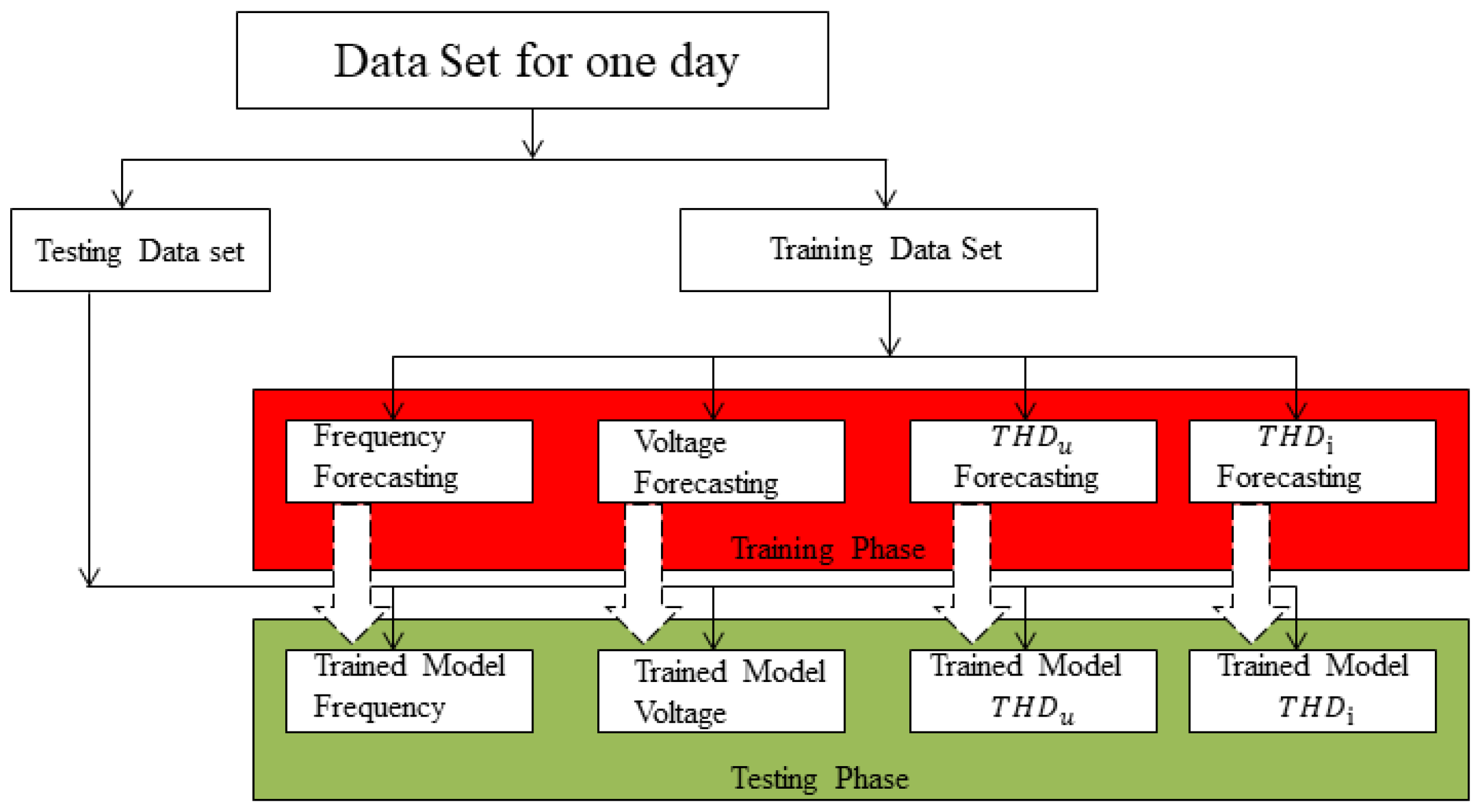
In our experiments, we compared the performance of seven approaches for PQP forecasting: the ANN, LR, ILR, PQLR, QLR, bagging DT, and boosting DT. The ANN was run in three configurations, i.e., two hidden layers with 10, 20, and 30 neurons in each layer. Two hidden layers with 20 neurons were chosen as the comparison model, because they afforded better results than the other two configurations. Linear regression was used with four different types of linear regression (LR): the linear (LR) system contains an intercept and linear term for each predictor; interactions (ILR) contains an intercept, linear term for each predictor, and all products of pairs of distinct predictors; pure quadratic (PQLR) contains an intercept term and linear and squared terms for each predictor; and quadratic (QLR) contains an intercept term, linear, and squared terms for each predictor, and all products of pairs of distinct predictors. Each designed model included four forecasting systems: power frequency, amplitude of voltage power, total harmonic distortion of voltage ($TH{D}_u$), and total harmonic distortion of current ($TH{D}_i$). Every system consists of multiple input variables (weather condition and load) and one output (frequency, voltage, $TH{D}_u$, or $TH{D}_i$). Therefore, every model has multiple inputs and multiple outputs. This is depicted in Figure 2, in Table 3, as well as in the structure of the dataset in Figure 3, and Figure 4 depicts the flowchart of the experiments. The dataset is then fed directly to the forecasting systems.

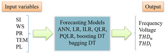
Figure 2. Scheme of the designed model. The input variables are solar irradiance (SI), wind speed (WS), air pressure (PR), air temperature (TEM), and power load (PL). The output are frequency, voltage, $TH{D}_u$, and $TH{D}_i$.

Table 3. Input and output variables.

Parameter	Parameter Details	Parameter Type
Gr	Global Solar Irradiance	Input
WS	Wind Speed	Input
Press	Air Pressure	Input
Tem	Air Temperature	Input
PL	Power Load	Input
Freq	Power Frequency	Output
V	Voltage Amplitude	Output
$TH{D}_u$	$THD$ of Voltage	Output
$TH{D}_i$	$THD$ of Current	Output

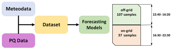
Figure 3. Structure of training and testing dataset.

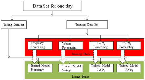
Figure 4. Flowchart of the designed model. The experiment procedure was done the same way as in this flowchart for all days and for all models.

The experiments were performed using EXCEL and MATLAB, according to the following steps:

• The dataset was prepared and cleaned using EXCEL.
• MATLAB code for reading the dataset, merging the power with weather data, and splitting the data into training and test datasets was designed.
• MATLAB code for the seven forecast models, plotting the results, and errors. Each model was designed separately, and all the models were subsequently combined into a single complex model using MATLAB.

These experiments were performed on a Lenovo computer with the following specifications: processor Intel(R) Pentium(R) CPU 5405U @ 2.30 GHz 2.30 GHz, installed RAM 4.00 GB (3.88 GB usable). The operating system used was Windows 11 Home, version 21H2. Programming language: MATLAB version R2018a.

5.1. Datasets

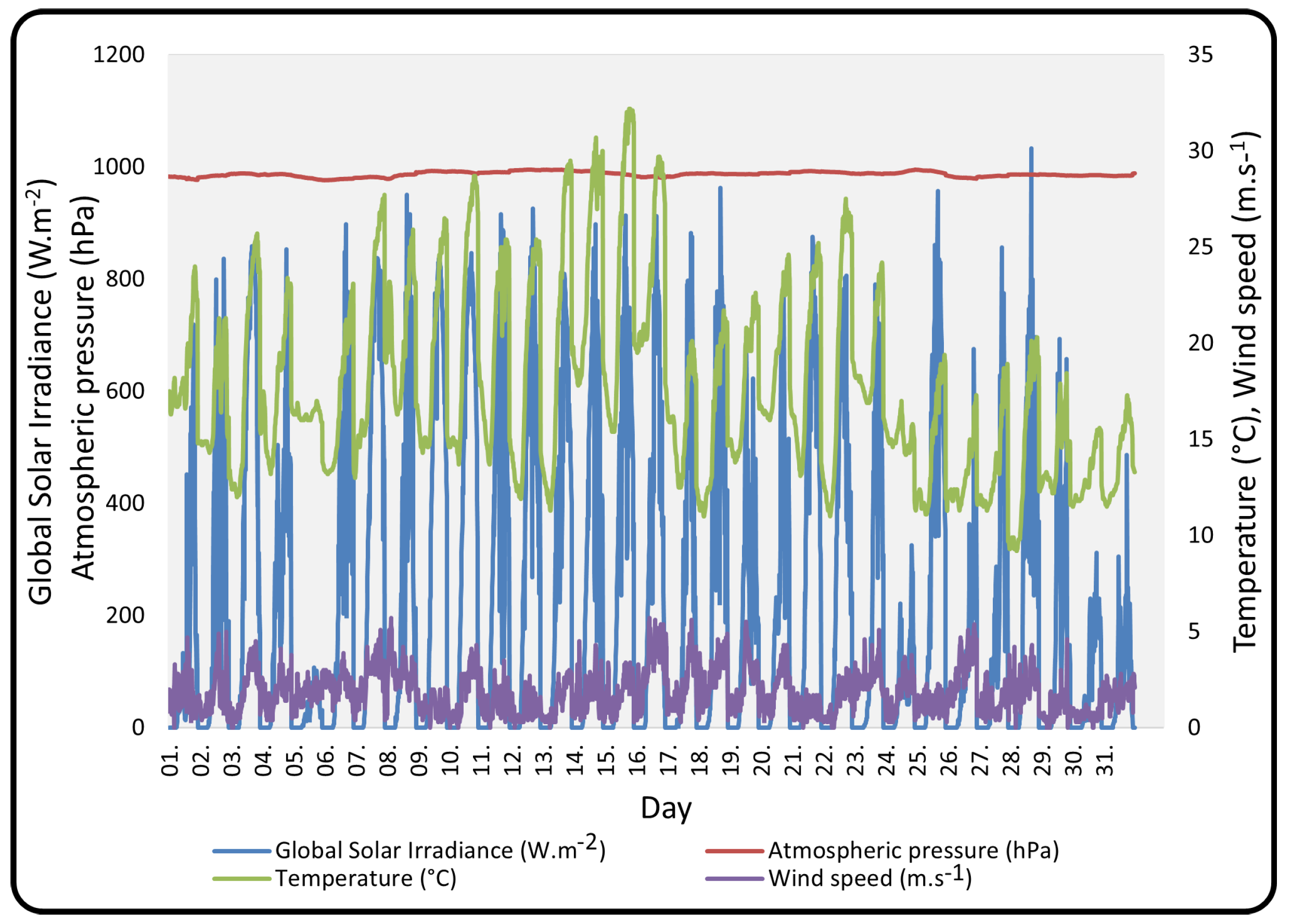
Figure 3 presents the structure of the dataset, and Figure 5 and Figure 6 show the weather conditions and PQPs values for August 2021, respectively. Table 4 and Table 5 present the weather dataset and PQP values. The datasets were obtained from two sources: the power dataset was obtained from the off-grid system installed at VSB-Technical University of Ostrava, whereas the weather dataset was obtained from the Czech Hydrometeorological Institute (CHMI) in Poruba, Ostrava. The off-grid system employed wind turbine and two solar panels; it supplied electricity to household appliances, acting as a load, and simultaneously recorded the state of these appliances when they were in operation or idle. In an off-grid system, weather conditions directly affect the PQPs, and the power quality is sensitive to the variations in the weather conditions [38]. In our experiments, all the input variables that directly affect the PQPs were selected to build the model. The selected input variables were: the global solar irradiance, wind speed, air pressure, air temperature, and power load, whereas the output PQPs were: the power frequency, the amplitude of power voltage, $TH{D}_u$, and $TH{D}_i$, as can be seen in Table 3.

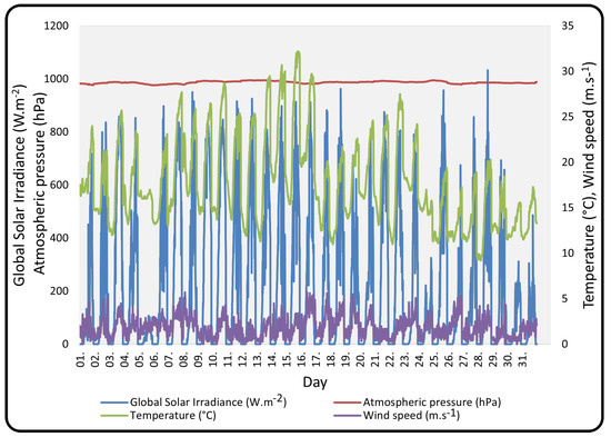
Figure 5. Variations in weather conditions in August 2021.

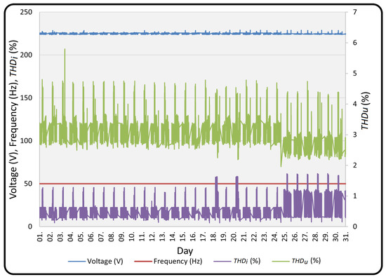
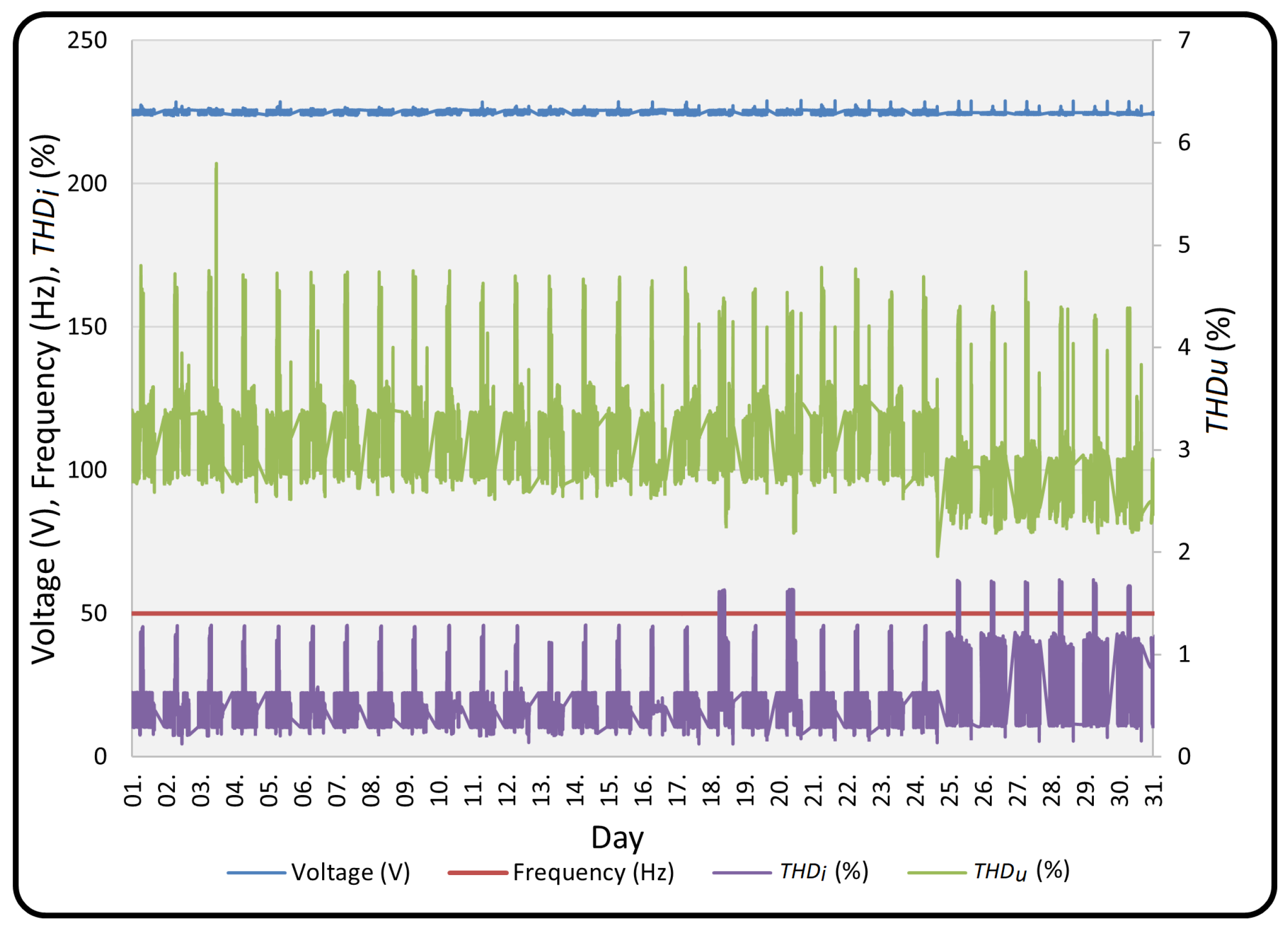
Figure 6. Variations in PQPs in August 2021.

Table 4. Weather dataset values.

Shortcut	Parameter	Min.	Max.	Avg.	Modus	Median
Gr	Global Solar Irradiance (W·m${}^{-2}$)	0	1033	227.02	0	89
Pr	Atmospheric Pressure (hPa)	976.4	995.3	987.07	988.5	987.2
Tem	Air Temperature (°C)	9.2	32.2	17.69	14.9	16.5
WS	Wind speed (m·s${}^{-1}$)	0	5.7	1.81	0.8	1.7

Table 5. PQPs dataset values.

Shortcut	Parameter	Min.	Max.	Avg.	Modus	Median
PL	Power Load (kW)	0.06	2.61	0.45	0.19	0.31
Freq	Frequency (Hz)	49.90	50.08	50.01	50.01	50.01
V	Voltage (V)	223.96	245.64	228.85	224.15	225.59
$TH{D}_u$	THD of voltage (%)	0.51	5.75	2.58	3.37	2.78
$TH{D}_i$	THD of current (%)	4.48	61.68	22.77	22.34	22.19

The August 2021 dataset (accessed on 1 April 2022) is available free of charge from the ENET Centre at this link (https://github.com/Sal0043?tab=projects). This dataset is available in two EXCEL formats: weather conditions and PQPs. Interested readers can download these data for scientific research.

5.2. Experimental Setup

The dataset used for the experiments contained data for August 2021. The off-grid system was connected to the external power grid from 16:30 to 22:30, which implies that it functioned as an on-grid system during this period. The weather dataset, collected by the Czech Hydrometeorological Institute (CHMI) located in Poruba, Ostrava, contained data measured at intervals of 10 min. The power dataset, collected using the off-grid system at the VSB- Technical University of Ostrava, contained data measured at intervals of 1 min. The power dataset adopted intervals of 10 min to match the weather dataset. Thus, for each day, 144 samples were acquired, which were then divided into two parts: the off-grid part, which included 107 samples, and the on-grid part, which included 37 samples. The experiments focused on the off-grid part of the system. This dataset of August 2021 was used to build our models. The dataset of the first two weeks of August was used for training, whereas the data for 16–18 August were used for forecasting and testing the models. Forecasting was performed hourly from 01:00 h until 16:00 h, thus, a total of 14 points were forecasted. This is depicted in the dataset in Figure 3.

6. Results

6.1. Forecasting Results

The most common metric for evaluating a forecasting model is the mean absolute percentage error (MAPE) [39,40,41] and was used to evaluate the forecasting results in this study. Table 6, Table 7, Table 8, Table 9, Table 10, Table 11 and Table 12 list the results for the: ANN, LR, ILR, QLR, PQLR, the boosting DT, and the bagging DT, respectively, for 16–18 August 2021. The average error was determined for each PQP. The residual results of the frequency, voltage, $TH{D}_u$, and $TH{D}_i$, for the training phase of the boosting DT and bagging DT are shown in Figure 7 and Figure 8, respectively.

Table 6. Forecasting error (MAPE in %) for 16–18 August 2021, when using ANN with two hidden layers and 20 neurons in each layer.

PQP Type	16th	17th	18th	Average
Frequency	$5.3\times {10}^{-4}$%	$1.88\times {10}^{-4}$%	$2.03\times {10}^{-4}$%	$3.09\times {10}^{-4}$%
Voltage	0.143%	0.08%	0.446%	0.223%
$TH{D}_u$	6.46%	4.16%	7.85%	5.15%
$TH{D}_i$	25.05%	14.55%	45.27%	20.85%

Table 7. Forecasting error (MAPE in %) for 16–18 August 2021, when using LR.

PQP Type	16th	17th	18th	Average
Frequency	$9.48\times {10}^{-5}$%	$4.55\times {10}^{-5}$%	$1.01\times {10}^{-4}$%	$8.16\times {10}^{-5}$%
Voltage	0.28%	0.335%	0.23%	0.28%
$TH{D}_u$	10.26%	12.72%	14.89%	12.62%
$TH{D}_i$	24.07%	49.85%	50.34%	41.42%

Table 8. Forecasting error MAPE (%) of 16–18 August 2021, using Interactions LR (ILR).

PQP Type	16th	17th	18th	Average
Frequency	$1\times {10}^{-4}$%	$4.4\times {10}^{-5}$%	$1\times {10}^{-4}$%	$8.13\times {10}^{-5}$%
Voltage	0.29%	0.34%	0.23%	0.28%
$TH{D}_u$	9.66%	12.74%	14.03%	12.14%
$TH{D}_i$	30.5%	52.9%	47.36%	43.58%

Table 9. Forecasting error (MAPE in%) for 16–18 August 2021, when using QLR.

PQP Type	16th	17th	18th	Average
Frequency	$1.08\times {10}^{-4}$%	$4.94\times {10}^{-5}$%	$1.04\times {10}^{-4}$%	$8.71\times {10}^{-5}$%
Voltage	0.22%	0.23%	0.16%	0.20%
$TH{D}_u$	12.22%	11.56%	12.11%	11.96%
$TH{D}_i$	28.61%	58.1%	47.58%	44.76%

Table 10. Forecasting error (MAPE in%) for 16–18 August 2021, when using PQLR.

PQP Type	16th	17th	18th	Average
Frequency	$9.33\times {10}^{-5}$%	$4.60\times {10}^{-5}$%	$1.01\times {10}^{-4}$%	$8.02\times {10}^{-5}$%
Voltage	0.20%	0.24%	0.180%	0.20%
$TH{D}_u$	11.29%	10.25%	11.96%	11.16%
$TH{D}_i$	27.68%	54.81%	47.36%	43.28%

Table 11. Forecasting error (MAPE in%) for 16–18 August 2021, when using the boosting DT.

PQP Type	16th	17th	18th	Average
Frequency	$1.35\times {10}^{-4}$%	$8.07\times {10}^{-5}$%	$1.53\times {10}^{-4}$%	$1.2\times {10}^{-4}$%
Voltage	0.054%	0.040%	0.094%	0.06%
$TH{D}_u$	4.39%	1.66%	5%	3.68%
$TH{D}_i$	4.86%	8.04%	20.79%	11.23%

Table 12. Forecasting error (MAPE in%) for 16–18 August 2021, when using the bagging DT.

PQP Type	16th	17th	18th	Average
Frequency	$9.35\times {10}^{-5}$%	$4.7\times {10}^{-5}$%	$1\times {10}^{-4}$%	$2.3\times {10}^{-4}$%
Voltage	0.10%	0.05%	0.051%	0.06%
$TH{D}_u$	3.00%	3.00%	5.00%	3.66%
$TH{D}_i$	5%	6.19%	19.23%	10.14%

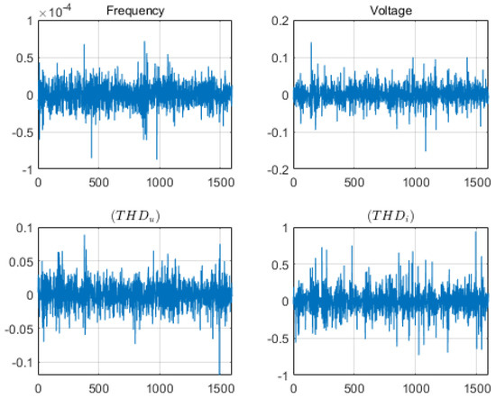
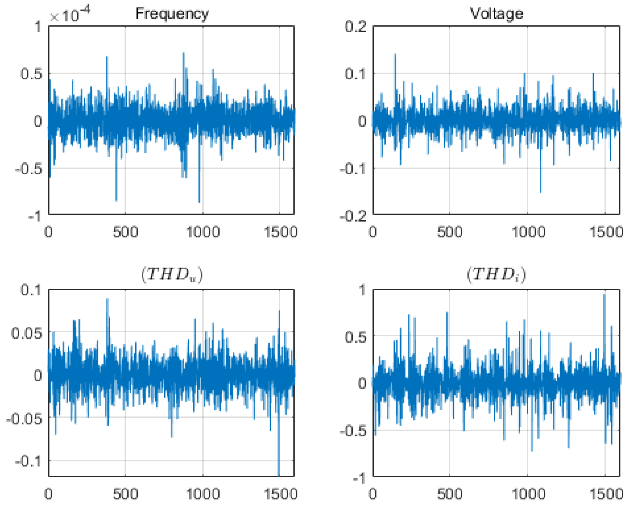
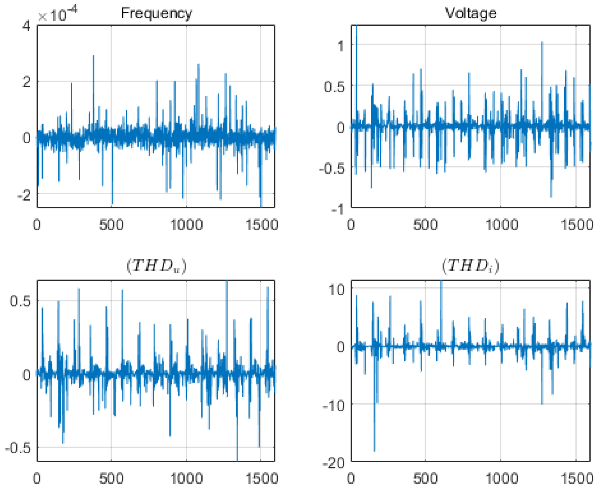
Figure 7. Residual results of the frequency, voltage, $TH{D}_u$, and $TH{D}_i$ of the training phase of boosting DT.

Figure 8. Residual results of the frequency, voltage, $TH{D}_u$, and $TH{D}_i$ of the training phase of bagging DT.

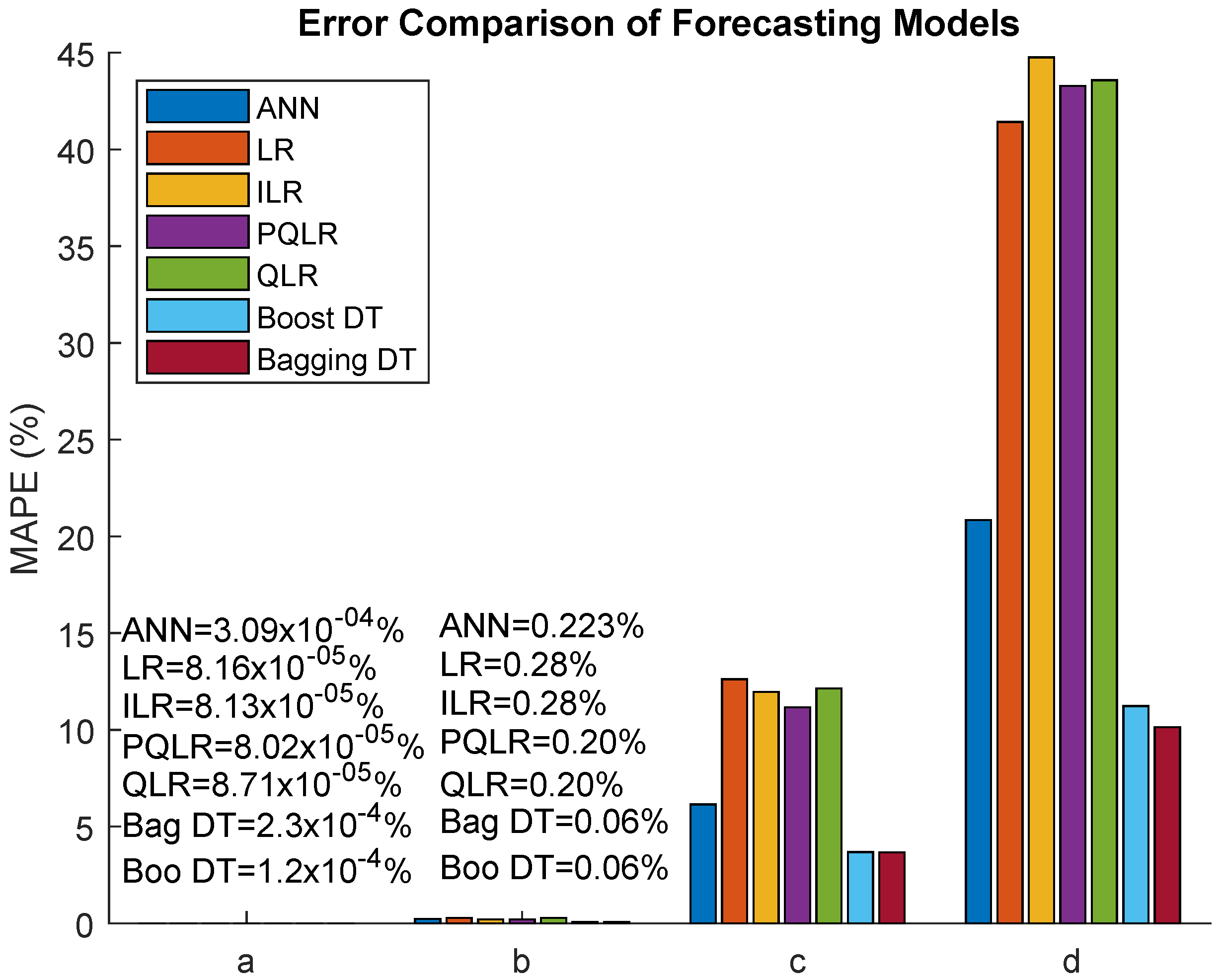
The average error of the ANN for the power frequency across these three days, with respect to voltage, $TH{D}_u$, and $TH{D}_i$, was approximately $3.09\times {10}^{-4}\%$, 0.223%, 5.15%, and 20.85%, respectively.

For LR, the average error in the frequency for all three days with respect to voltage, $TH{D}_u$, and $TH{D}_i$ was approximately $8.16\times {10}^{-5}\%$, 0.28%, 12.62%, and 41.42%, respectively. For ILR, the average error in the frequency for all three days with respect to voltage, $TH{D}_u$, and $TH{D}_i$ was approximately $8.13\times {10}^{-5}\%$, 0.28%, 12.14%, and 43.58%, respectively. For QLR, the average error in the frequency for all three days with respect to voltage, $TH{D}_u$, and $TH{D}_i$ was approximately $8.71\times {10}^{-5}\%$, 0.20%, 11.96%, and 44.76%, respectively.

For PQLR, the average error in the frequency for all three days with respect to voltage, $TH{D}_u$, and $TH{D}_i$ was approximately $8.02\times {10}^{-5}\%$, 0.20%, 11.16%, and 43.28%. respectively. For the bagging DT, the average error in the frequency for all three days, with respect to voltage, $TH{D}_u$, and $TH{D}_i$ was approximately $2.3\times {10}^{-4}\%$, 0.06%, 3.66%, 10.14% respectively.

For the boosting DT, the average error in the frequency for all three days, with respect to voltage, $TH{D}_u$, and $TH{D}_i$, was approximately $1.2\times {10}^{-4}\%$, 0.06%, 3.68%, 11.23% respectively.

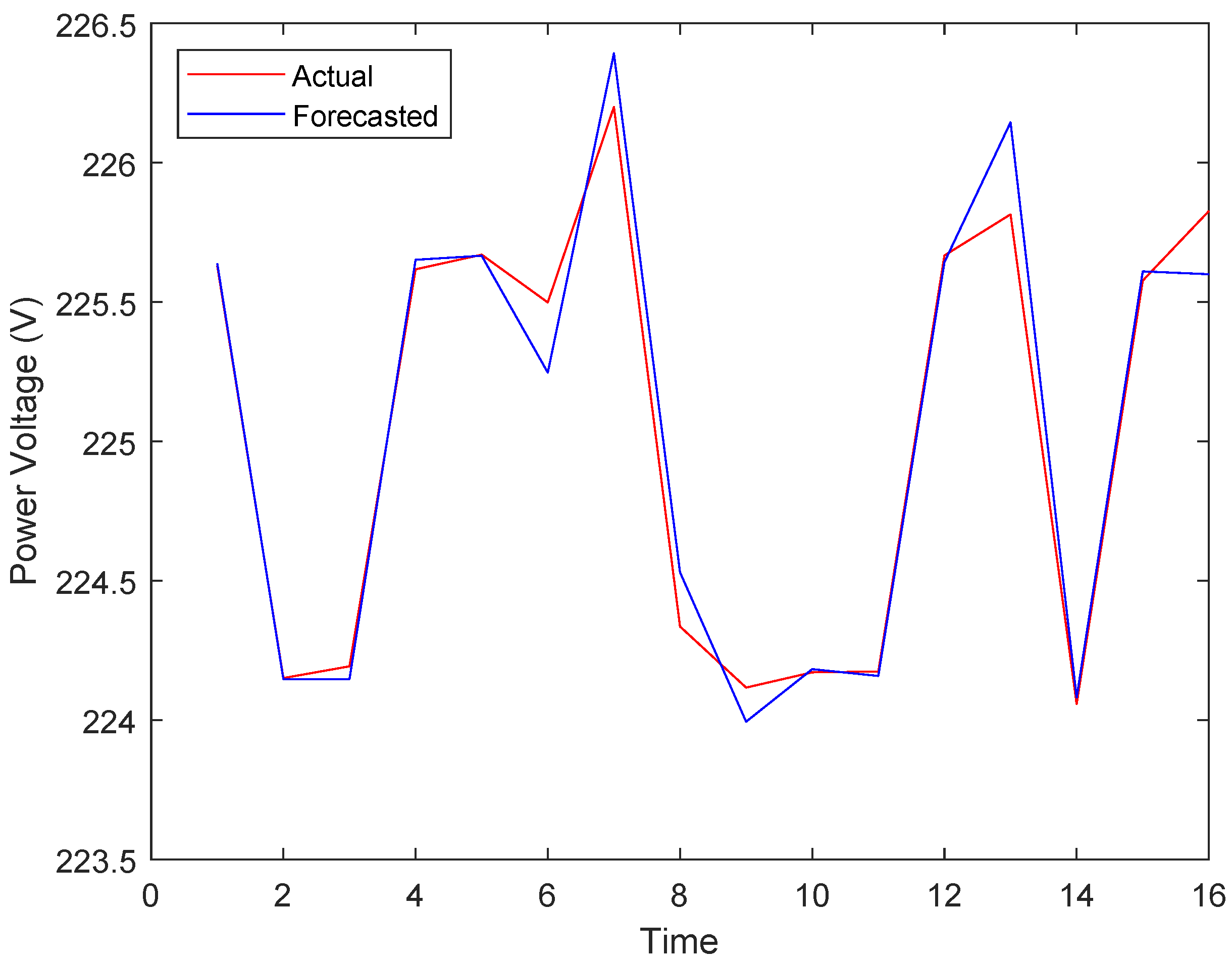
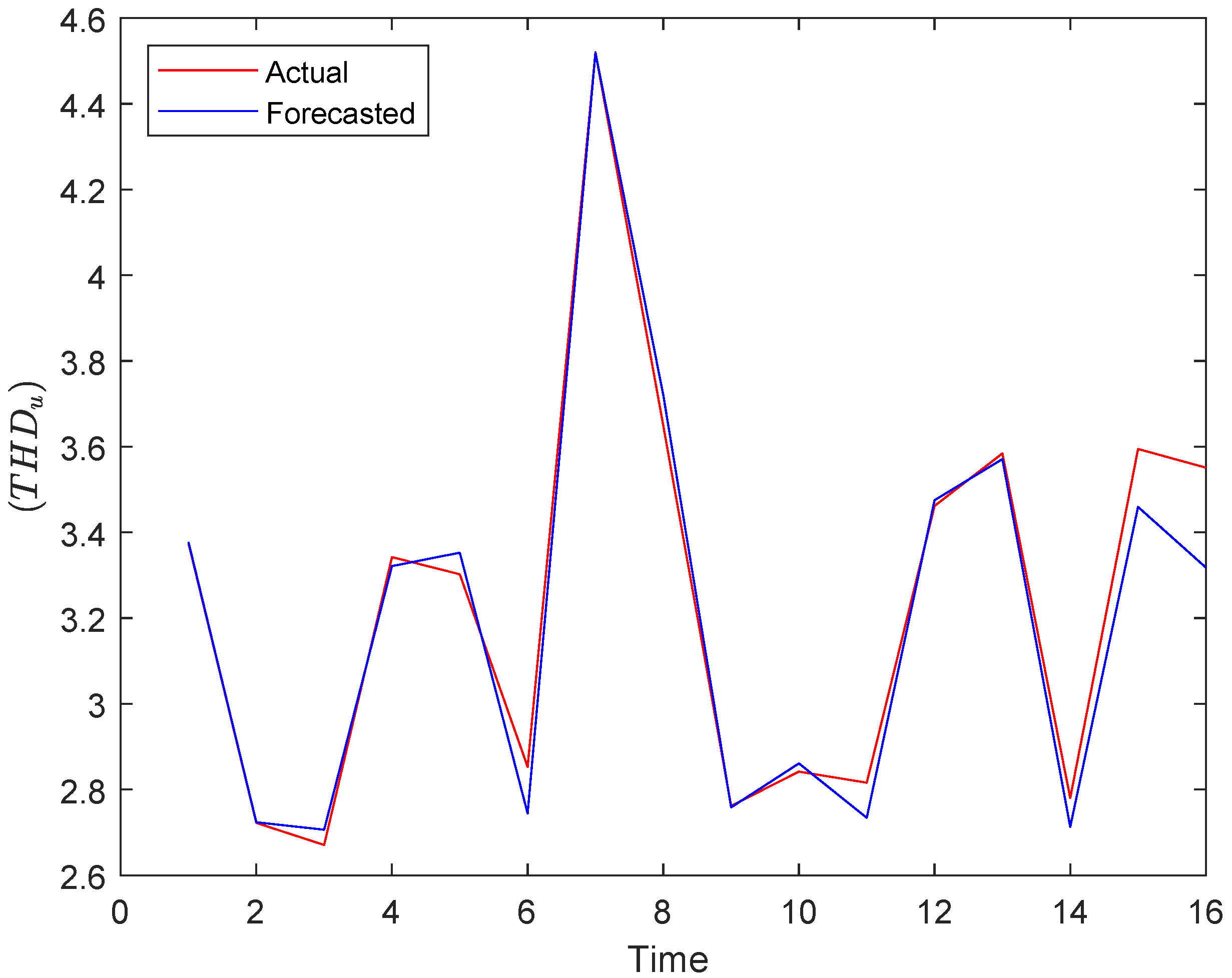
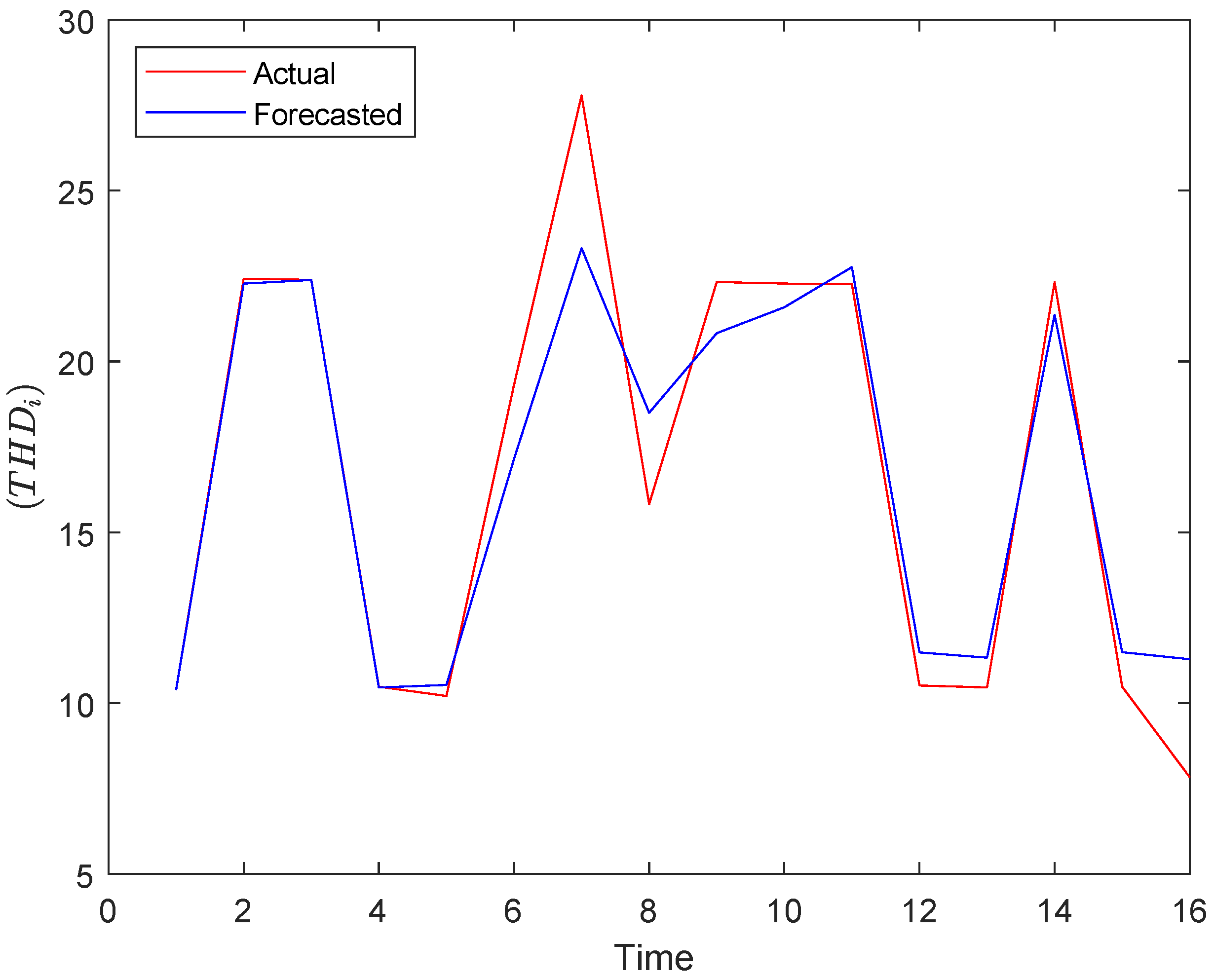
As the difference between the actual and forecasted frequencies was significantly small, the curves plotted using these values appear identical. Comparisons between the actual and forecasted values of voltage, $TH{D}_u,TH{D}_i$ when using the regression tree are presented in Figure 9, Figure 10 and Figure 11, respectively.

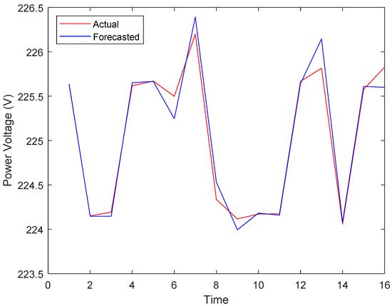
Figure 9. Comparison of actual and forecasted voltage when using DT.

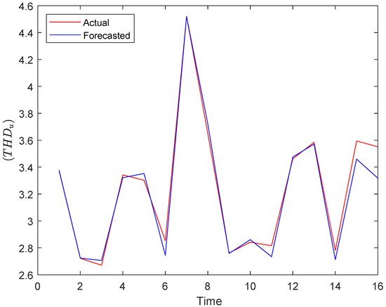
Figure 10. Comparison of actual and forecasted $TH{D}_u$ when using DT.

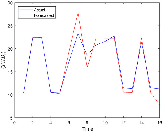
Figure 11. Comparison of actual and forecasted $TH{D}_i$ when using DT.

6.2. Computational Time

Table 13 lists the approximate computational times required for the tests performed in this study. The execution time for forecasting all four PQPs ranged from 47.81 to 56.76 s for ANN, from 4.12 to 4.75 s for the LR variations, from 11.10 to 10.50 s for the bagging DT, and from 9.04 to 9.51 s for the boosting DT.

Table 13. Approximate computational times for different models.

Model	Day
	16th	17th	18th
ANN	47.81 s	56.76 s	49.47 s
LR	4.19 s	4.19 s	4.12 s
ILR	4.40 s	4.37 s	4.75 s
PQLR	4.22 s	4.22 s	4.64 s
QLR	4.44 s	4.35 s	4.30 s
Boosting DT	9.04 s	9.51 s	9.45 s
Bagging DT	10.16 s	10.50 s	11.10 s

7. Discussion

7.1. Forecasting Comparison

A comparison of the forecasting results from the seven models is presented in Table 14 and Figure 12; these explain the results of the average error for the compared models. The power frequency appears to remain constant; the maximum value of the power frequency was 50.0076 Hz, whereas its minimum value was 50.0069 Hz. Hence, the power frequency forecasts obtained using the bagging and boosting DTs had little more error than those from the other models. The experiment focused on the power consumption and generation for a typical small household, considering an off-grid system. This is associated with a lower short circuit power. As a result, devices in smaller off-grid systems have a greater impact on the power quality than appliances connected to the distribution grid. The power quality in an off-grid system is largely determined by the inverter’s ability to handle the influence of the appliances. This results in significant total harmonic distortion in these systems. None of the existing standards apply to small, private off-grid systems. Hence, this work was aimed at predicting such situations in order to ensure appropriate responses in advance. The results show that the the total harmonic distortion values are complicated to predict. Furthermore, the dataset and results indicate that the larger the range of power quality values, the lower the prediction accuracy is. When measuring the individual appliances, we found that the lamps and the microwave oven have the greatest impact on the total harmonic distortion in our chosen off-grid system. Overall, the best forecasting results for the power frequency were obtained using PQLR, followes by those afforded by ILR, LR, QLR, the boosting and bagging DTs, and the ANN, respectively. With regard to the voltage, the best results were obtained using the bagging and boosting DTs, followed by those from PQLR and QLR, the ANN, and LR and ILR, respectively. For $TH{D}_u$ and $TH{D}_i$ parameters, the good results were achieved by bagging DT, and boosting DT ranked second, then ANN, and the worst results were achieved by variations of LR models. Based on the results, as mentioned earlier, the frequency patterns appear identical, and the bagging and boosting DTs involve smaller errors than the other models. However, among the PQPs, the best voltage forecasts were afforded by the bagging DT, followed by those from the boosting DT; additionally, these results were better than those of the other models.

Table 14. Average error for 16–18 August 2021, obtained when using the ANN, LR, ILR, QLR, PQLR, the boosting DT, and the bagging DT.

PQP Type	Model
	ANN	LR	ILR	QLR	PQLR	Boosting DT	Bagging DT
Frequency	$1.08\times {10}^{-4}$%	$8.16\times {10}^{-5}$%	$8.13\times {10}^{-4}$%	$8.7\times {10}^{-5}$%	$8.02\times {10}^{-5}$%	$1.2\times {10}^{-4}$%	$2.3\times {10}^{-4}$%
Voltage	0.22%	0.28%	0.28%	0.20%	0.20%	0.06%	0.06%
$TH{D}_u$	12.22%	12.62%	12.14%	11.96%	11.16%	3.68%	3.66%
$TH{D}_i$	28.61%	41.42%	43.58%	44.76%	43.28%	11.23%	10.14%

Figure 12. Comparison of the error results for the forecasting models, a, b, c, d for frequency, voltage, $THDu$, and $THDi$, respectively.

7.2. Comparison of Model Performance

In this work, we applied bagging and boosting DTs, which are relatively new techniques. The performance of these methods was compared with that of the other traditional methods, such as the ANN and LR. In our experiments, we developed seven complex models for forecasting four PQPs. We used weather and power load data to build these models.

Because the PQPs are very sensitive to the power load, they can be affected by weather conditions [38]. Our experiments were tested for three days ahead and considered the forecasting error and the execution time of tested models. In reference [15] home appliances and PQPs were used to forecast future PQPs, and in [16] the experiments tested for one day ahead. One of the advantages of the ANN is that it can be configured in many forms; however, it requires a significant amount of time for learning. LR is a considerably simple model and exhibits shorter computational times; however, it suffers from limitations in dealing with nonlinear data. When using ILR, the effect of one feature on the forecasted value is dependent on the other features; however, these interactions can increase the noise in the data and the learning time, especially for higher-order interactions. PQLR can handle nonlinear data but requires additional data points. Furthermore, the QLR interaction affects the results, in addition to the effects of individual features, and requires additional data points with a higher order of interactions; this may lead to an increase in the learning time. The boosting DT is capable of handling missing values and requires less computational time, as compared with the other models; however, in certain cases, overfitting can occur. The bagging DT can handle missing data, but the final results depend on the average of the sub-trees outputs. Table 15 presents the advantages and disadvantages of the models used in this study.

Table 15. Approximation of comparison of the used models.

Model Type	Advantage	Disadvantage
ANN	It can be set up in different configurations	Longer computation time
LR	Very simple and fast in computing	Difficulty in dealing with nonlinear data
ILR	The effect of one feature on the forecasted result is dependent on the remaining features	Interactions can increase the noise in data and computation time of higher-order interactions
PQLR	It handles nonlinear data	More data points required
QLR	It is suitable for nonlinear data. The effect of one feature on the forecasted result is dependent on the remaining features	More data points and longer computational time are required
Boosting DT	It handles missing data and takes less time compared with bagging DT	Longer computation time compared with LR versions
Bagging DT	It handles higher dimensional data handles missing data	The final results are based on mean average results from sub trees, which does not render precise forecasting values

8. Conclusions

In summary, this study compared seven forecasting models for the PQPs of small-scale household off-grid systems. The models considered were the ANN, DTs, LR, ILR, QLR, and PQLR. Furthermore, with regard to the PQPs, we emphasised the power frequency, voltage, total harmonic distortion voltage and current. In addition, the MAPE was used to compare and evaluate the performance of these forecasting systems. The power frequency is given that shows the model’s prediction on minimal values of the differences. These minor differences are smaller than the measurement error. The article used frequency to show how the different models deal with this. The experimental results of the study can be summarised as follows:

• The best voltage forecasting accuracy was achieved by the bagging and boosting DTs (approximately 0.06%), followed by those of QLR (approximately 0.20%), PQLR, LR, and ILR, respectively. In this case, the worst results were afforded by the by ANN.
• The boosting DT achieved the best forecasting accuracy of $TH{D}_u$ (3.68%), followed by the bagging DT (3.66%) and the ANN. The lower accuracies were afforded by the LR models (11.16% to 12.62%).
• The best forecasting accuracy results of $TH{D}_i$ were achieved by the bagging DT (approximately 10.14%), followed by the boosting DT (11.23%) and the ANN; the worst forecasting results were yielded by the LR model (41.42%).
• With regard to frequency, the best forecasting accuracy results were achieved by PQLR, followed by those from ILR, LR, QLR, the boosting DT, the bagging DT, and the ANN, respectively.
• The ANN required more computational time than the other models (47.81 s to 56.76 s). By contrast, the LR models required the shortest computational times (4.12 to 4.44 s). Furthermore, the bagging DT required 10.10 to 10.50 s, and the boosting DT required 9.04 to 9.51 s.

These experimental results are expected to be used for developing off-grid control systems. In addition, these prediction models can contribute toward optimisation processes that ensure the appropriate operation of the entire system. The results of this work can also be used to develop more in-depth power quality parameter forecasting methods to improve their accuracy for small-household off-grid systems. The study dealt with forecasting power quality parameters based on meteorological data in Central Europe. Different results may come out in other parts of the world under different climatic conditions and experimental infrastructure. The study was mainly concerned with the presentation and application of the idea. In the future, we plan to apply these methods to large-scale off-grid systems, such as municipal buildings or industrial facilities cooperating with the vehicle-to-grid technology.

References

- Kosmak, J.; Misak, S. Power quality management in an off-grid system. In Proceedings of the 2018 IEEE International Conference on Environment and Electrical Engineering and 2018 IEEE Industrial and Commercial Power Systems Europe (EEEIC/I&CPS Europe), Palermo, Italy, 12–15 June 2018; pp. 1–5. [Google Scholar]
- European Std Committee EN 50160-2002; Voltage Characteristics of Electricity Supplied by Public Distribution Systems. BSI Standards Limited: London, UK, 2003.
- Jahan, I.S.; Misak, S.; Snasel, V. Smart control system based on power quality parameter short-term forecasting. In Proceedings of the 2020 21st International Scientific Conference on Electric Power Engineering (EPE), Prague, Czech Republic, 19–21 October 2020; pp. 1–5. [Google Scholar]
- Misak, S.; Stuchly, J.; Vantuch, T.; Burianek, T.; Seidl, D.; Prokop, L. A holistic approach to power quality parameter optimization in ac coupling off-grid systems. Electr. Power Syst. Res. 2017, 147, 165–173. [Google Scholar] [CrossRef]
- Blazek, V.; Petruzela, M.; Vysocky, J.; Prokop, L.; Misak, S.; Seidl, D. Concept of real-time communication in off-grid system with vehicle-to-home technology. In Proceedings of the 2020 21st International Scientific Conference on Electric Power Engineering (EPE), Prague, Czech Republic, 19–21 October 2020; pp. 1–6. [Google Scholar]
- Kosinka, M.; Slanina, Z.; Petruzela, M.; Blazek, V. V2h control system software analysis and design. In Proceedings of the 2020 20th International Conference on Control, Automation and Systems (ICCAS), Busan, Korea, 13–16 October 2020; pp. 972–977. [Google Scholar]
- Slanina, Z.; Docekal, T. Energy meter for smart home purposes. In International Conference on Intelligent Information Technologies for Industry; Springer: Cham, Switzerland; Varna, Bulgaria, 2017; pp. 57–66. [Google Scholar]
- Blazek, V.; Petruzela, M.; Vantuch, T.; Slanina, Z.; Misak, S.; Walendziuk, W. The estimation of the influence of household appliances on the power quality in a microgrid system. Energies 2020, 13, 4323. [Google Scholar] [CrossRef]
- Jahan, I.S.; Snasel, V.; Misak, S. Intelligent systems for power load fore casting: A study review. Energies 2020, 13, 6105. [Google Scholar] [CrossRef]
- Vantuch, T.; Misak, S.; Jezowicz, T.; Burianek, T.; Snasel, V. The power quality forecasting model for off-grid system supported by multiobjective optimization. IEEE Trans. Ind. Electron. 2017, 64, 9507–9516. [Google Scholar] [CrossRef]
- Jahan, I.S.; Misak, S.; Snasel, V. Power quality parameters analysis in off-grid platform. In International Conference on Intelligent Information Technologies for Industry; Springer: Sirius, Russia, 2021; pp. 431–439. [Google Scholar]
- Stuchly, J.; Misak, S.; Vantuch, V.; Burianek, T. A power quality forecasting model as an integrate part of active demand side management using artificial intelligence technique-multilayer neural network with backpropagation learning algorithm. In Proceedings of the 2015 IEEE 15th International Conference on Environment and Electrical Engineering (EEEIC), Rome, Italy, 10–13 June 2015; pp. 611–616. [Google Scholar]
- Rodway, J.; Musilek, P.; Misak, S.; Prokop, L. Prediction of pv power quality: Total harmonic distortion of current. In Proceedings of the 2013 IEEE Electrical Power & Energy Conference, Halifax, NS, Canada, 21–23 August 2013; pp. 1–4. [Google Scholar]
- Vantuch, T.; Misak, S.; Stuchly, J. Power quality prediction designed as binary classification in ac coupling off-grid system. In Proceedings of the 2016 IEEE 16th international Conference on Environment and Electrical Engineering (EEEIC), Florence, Italy, 7–10 June 2016; pp. 1–6. [Google Scholar]
- Zjavka, L. Power quality multi-step predictions with the gradually increasing selected input parameters using machine-learning and regression. Sustain. Energy Grids Netw. 2021, 26, 100442. [Google Scholar] [CrossRef]
- Zjavka, L. Power quality statistical predictions based on differential, deep and probabilistic learning using off-grid and meteo data in 24-hour horizon. Int. J. Energy Res. 2021, 46, 10182–10196. [Google Scholar] [CrossRef]
- Eisenmann, A.; Streubel, T.; Rudion, K. Power quality prediction by way of parallel computing-a new approach based on a long short-term memory network. In Proceedings of the 2019 IEEE PES Innovative Smart Grid Technologies Europe (ISGT-Europe), Bucharest, Romania, 29 September–2 October 2019; pp. 1–5. [Google Scholar]
- Sarkar, D.; Gunturi, S.K. Machine learning enabled steady-state security predictor as deployed for distribution feeder reconfiguration. J. Electr. Eng. Technol. 2021, 16, 1197–1206. [Google Scholar] [CrossRef]
- Kahouli, O.; Alsaif, H.; Bouteraa, Y.; Ben Ali, N.; Chaabene, M. Power system reconfiguration in distribution network for improving reliability using genetic algorithm and particle swarm optimization. Appl. Sci. 2021, 11, 3092. [Google Scholar] [CrossRef]
- Atteya, I.I.; Ashour, H.A.; Fahmi, N.; Strickland, D. Distribution network reconfiguration in smart grid system using modified particle swarm optimization. In Proceedings of the 2016 IEEE International Conference on Renewable Energy Research and Applications (ICRERA), Birmingham, UK, 20–23 November 2016; pp. 305–313. [Google Scholar]
- Fathabadi, H. Power distribution network reconfiguration for power loss minimization using novel dynamic fuzzy c-means (dfcm) clustering based ANN approach. Int. J. Electr. Power Energy Syst. 2016, 78, 96–107. [Google Scholar] [CrossRef]
- Nguyen, T.T.; Truong, A.V. Distribution network reconfiguration for power loss minimization and voltage profile improvement using cuckoo search algorithm. Int. J. Electr. Power Energy Syst. 2015, 68, 233–242. [Google Scholar] [CrossRef]
- Reddy, A.V.S.; Reddy, M.D.; Reddy, M.S.K. Network reconfiguration of distribution system for loss reduction using gwo algorithm. Int. J. Electr. Comput. Eng. 2017, 7, 3226–3234. [Google Scholar]
- Ji, X.; Yin, Z.; Zhang, Y.; Xu, B.; Iiu, Q. Real-time autonomous dynamic reconfiguration based on deep learning algorithm for distribution network. Electr. Power Syst. Res. 2021, 195, 107132. [Google Scholar] [CrossRef]
- Salau, A.O.; Gebru, Y.W.; Bitew, D. Optimal network reconfiguration for power loss minimization and voltage profile enhancement in distribution systems. Heliyon 2020, 6, e04233. [Google Scholar] [CrossRef]
- Ramadan, H.S.; Helmi, A.M. Optimal reconfiguration for vulnerable radial smart grids under uncertain operating conditions. Comput. Electr. Eng. 2021, 93, 107310. [Google Scholar] [CrossRef]
- Oh, S.H.; Yoon, Y.T.; Kim, S.W. Online reconfiguration scheme of selfsufficient distribution network based on a reinforcement learning approach. Appl. Energy 2020, 280, 115900. [Google Scholar] [CrossRef]
- Essallah, S.; Khedher, A. Optimization of distribution system operation by network reconfiguration and dg integration using mpso algorithm. Renew. Energy Focus 2020, 34, 37–46. [Google Scholar] [CrossRef]
- Tran, T.T.; Truong, K.H.; Vo, D.N. Stochastic fractal search algorithm for reconfiguration of distribution networks with distributed generations. Ain. Shams Eng. J. 2020, 11, 389–407. [Google Scholar] [CrossRef]
- Sambaiah, K.S.; Jayabarathi, T. Optimal reconfiguration and renewable distributed generation allocation in electric distribution systems. Int. J. Ambient. Energy 2021, 42, 1018–1031. [Google Scholar] [CrossRef]
- Forcan, J.; Forcan, M. Optimal placement of remote-controlled switches in distribution networks considering load forecasting. Sustain. Energy Grids Netw. 2022, 30, 100600. [Google Scholar] [CrossRef]
- Misak, S.; Stuchly, J.; Vramba, J.; Prokop, L.; Uher, M. Power quality analysis in off-grid power platform. Adv. Electr. Electron. Eng. 2014, 12, 177–184. [Google Scholar] [CrossRef]
- BS. Institution. Electromagnetic Compatibility (EMC)—Part 6-1: Generic Standards—Immunity Standard for Residential, Commercial and Light Industrial Environments; BSI Standards Limited: London, UK, 2010. [Google Scholar]
- Zurada, J. Introduction to Artificial Neural Systems; West Publishing, Co., Ltd.: St. Paul, MN, USA, 1992. [Google Scholar]
- James, G.; Witten, D.; Hastie, T.; Tibshirani, R. An Introduction to Statistical Learning; Springer: New York, NY, USA, 2013. [Google Scholar]
- Jaccard, J.; Turrisi, R.; Jaccard, J. Interaction Effects in Multiple Regression; Sage: New York, NY, USA, 2003. [Google Scholar]
- Breiman, L. Random forests. Mach. Learn. 2001, 45, 5–32. [Google Scholar] [CrossRef] [Green Version]
- Burianek, T.; Vantuch, T.; Stuchly, J.; Misak, S. Off-grid parameters analysis method based on dimensionality reduction and self-organizing map. In International Conference on Soft Computing-MENDEL; Springer: Cham, Switzerland, 2016; pp. 235–244. [Google Scholar]
- Almeshaiei, E.; Soltan, H. A methodology for electric power load forecasting. Alex. Eng. J. 2011, 50, 137–144. [Google Scholar] [CrossRef] [Green Version]
- Weron, R. Modeling and Forecasting Electricity Loads and Prices: A Statistical Approach; John Wiley & Sons: Chichester, UK, 2007. [Google Scholar]
- Palit, A.K.; Popovic, D. Computational Intelligence in Time Series Forecasting: Theory and Engineering Applications; Springer Science & Business Media: London, UK, 2006. [Google Scholar]
Publisher’s Note: MDPI stays neutral with regard to jurisdictional claims in published maps and institutional affiliations. |
© 2022 by the authors. Licensee MDPI, Basel, Switzerland. This article is an open access article distributed under the terms and conditions of the Creative Commons Attribution (CC BY) license (https://creativecommons.org/licenses/by/4.0/).