Refined 1D–3D Coupling for High-Frequency Forced Vibration Analysis in Hydraulic Systems

Abstract

High-Frequency Pressure Fluctuation (HFPF) is an extensively observed hydraulic phenomenon in pumped-storage power stations and water conveyance projects. The investigation of the propagation characteristics of the pressure perturbation is of great significance for the safe operation of hydraulic facilities. In this study, a one-dimensional (1D)–three-dimensional (3D) coupling model is established based on the combination of the Method of Characteristics (MOC) and Computational Fluid Dynamics (CFD) and implanted in the open source software OpenFOAM. The established model in this study implants the dynamic mesh module into the original OpenFOAM solver sonicLiquidFoam and presents the complete solution procedure of the CFD model with the dynamic mesh considered. The vibration of the pipe walls modeled by the mesh motion is employed to numerically generate the HFPF in the hydraulic system, which could not be implemented in the traditional MOC model. The independence of the pressure perturbation in the pipeline system is validated by the time-domain pressure variation. The graphical method is applied to describe the multiple reflection and superposition characteristics of the traveling wave in a simplified hydraulic system. Based on this, the mechanism of the superimposed characteristic of the traveling and standing pressure waves in the hydraulic system are analyzed, and the theoretical superimposed time-domain processes and the variations of the pressure oscillation magnitude are analyzed and presented. The 1D–3D coupling method and the theoretical analysis method could be referenced by other complex hydraulic systems.

1. Introduction

Pressure pulsation and forced vibration are frequently observed phenomena in hydropower plants and water conveyance projects. The existence of the pressure pulsation may induce the vibration of the structure containing it and compromise the safety operation condition of the hydraulic facilities [1,2,3]. The High-Frequency Pressure Fluctuation (HFPF) may also cause unignorable noise pollution [4,5,6] in an extensive range via the propagation of water hammers in the pressurized conduct. Therefore, the investigation of the HFPF is essential to guarantee the safety and normal operating condition of the hydraulic facilities.

The vibration sources in the hydropower plants are diversified, and most of them are related to the existence of the hydro-turbines [7,8,9,10], e.g., vortex rope in the draft tube, rotating stall in the pump-turbine, pressure fluctuation in the S-shape region, etc. The acoustic perturbation due to the instability of the vibration sources could also induce hydraulic forced vibration [11,12,13] in the conveyance conduit via the propagation of the water hammer. At resonance, the superimposition of the traveling and standing pressure waves leads to vibration with enlarged amplitudes along the entire conveyance conduits [14]. On the other hand, the energy contained in the fluid is passed to the walls of the pipes, resulting in decreased efficiency and increasing the risk of pipeline bursts.

Several one-dimensioned (1D) methods have been employed to analyze the forced vibration phenomenon in the hydraulic system, including the Method of the Characteristics (MOC) and the combination of the impedance method and transfer matrix method [15]. The former focus on the time-domain transient process, and the latter uses the frequency-domain method [16] to investigate the steady oscillatory conditions. The global matrix method [17] is proposed to conveniently establish the theoretical model of the complex system for hydraulic vibration analysis. However, almost all 1D algorithms encounter the overdetermined numerical dilemma [18,19] for the forced vibration analysis caused by the unbalanced governing equations and the unknown variables. For the MOC method, the unknown variables are discharge and pressure, while the equations contain two characteristic equations and one explicit equation provided by the characteristic of the vibration source. As for the frequency-domain method, the absolute pressure and discharge oscillation could not be closed by the reservoir boundaries. The main reason for the overdetermined problem is the neglect of the multiple reflection and superposition characteristics of the traveling wave [20,21,22]. A reliable method for overcoming the overdetermined problem is by employing the three-dimensional (3D) Computational Fluid Dynamics (CFD) method.

Several researchers recommended employing the CFD method to model the vibration sources with more convenience to observe and analyze the formation mechanism of the vibration sources [23,24]. Nevertheless, the computational consumption of the CFD approach is usually expensive, especially for the extensive hydraulic system. As a compromise, the 1D–3D coupling method is suggested to save computational resources, where the complex vibration region is handled by the CFD method, and it is suggested to utilize the MOC method to manage other parts of the system with long conveyance conduits [25,26,27,28]. However, unreasonable numerical attenuation is observed in the CFD part when the HFPF occurs in the system, which is mainly caused by the limitation of the CFD method when dealing with the large density gradient. Therefore, employing the coupling of 1D–3D could help minimize the inaccurate numerical flaws and decrease the computational requirements.

The 1D–3D coupling method has been applied in plenty of research fields. For the coupling problems, two coupling strategies could be recognized, e.g., fully coupling or partly coupling. All the variables in the interface are taken into consideration for the former coupling method. Several researchers employed the full coupling strategy to solve the transient multi-physics coupling problems [29,30,31]. On the contrary, only the dominant variables are utilized in the latter. Meanwhile, the focused contents in the water hammer phenomenon and forced vibration analysis are the magnitude and frequency of the pressure fluctuation. Therefore, only the pressure and velocity are considered in the coupling interface, and the influence of the energy equation and turbulent model is neglected in this study.

The most crucial arrangement in the 1D–3D coupling method is the management of the coupling boundaries, which determines the performance of the results to a large degree. Several methods have been proposed for deriving the coupling boundaries. Yang [32,33] presents a trial method for deriving the coupling boundary conditions. The initial assumed uniform velocity is first given to the CFD program, and the CFD procedure executes one step to return the boundary pressure. Then, the MOC corrects the coupling velocity according to the produced boundary pressure from the CFD program by either characteristics equation. After that, the new velocity of the coupling boundary is provided to the CFD program and trialed again until the velocity and pressure are satisfied for both the MOC and CFD procedures. Ruprecht [34,35] employs a simplified trial method, where the pressure at the coupling boundary is first assumed, and uses one trial of the CFD program to derive the pressure and velocity of the coupling boundary and then apply it to the CFD and MOC programs. Zhang [36] presents two strategies for the coupling boundary, named Partly Overlapped Coupling (POC) and Adjacent Coupling (AC). In the POC method, the simulation domain of MOC and CFD parts are overlapped for one space step. The boundary of the MOC part could be derived from the results of CFD at time n. Then, the MOC procedure is executed to obtain the fields at time n + 1. Finally, the boundary of CFD, which is overlapped in the MOC domain, could be obtained from MOC results at time n + 1. In the AC method, the adjacent node of the coupling boundary in the CFD part is utilized to construct an auxiliary equation, named the unsteady Bernoulli equation, to derive the discharge at time n + 1. Then, the pressure of the coupling boundary could be obtained by the characteristic equation of the MOC part. Wang [37] deduced the auxiliary equations in the CFD part based on Riemann invariants and implemented them in OpenFOAM. The auxiliary equations are similar to the characteristic equations and could be utilized to explicitly obtain the pressure and discharge at the coupling boundaries with the collaboration of the equations derived from MOC.

In this study, the coupling strategy proposed by Wang [37] is employed due to the efficiency and the concision characteristics. Furthermore, several numerical flaws in the coupling of 1D–3D are discussed, and corresponding solutions are discussed. Based on the coupling method, the high-frequency forced vibration in the hydraulic system is modeled, where the pipe vibration is simulated as the vibration source. The remainder of this paper is structured as follows. In Section 2, the basic governing and 1D–3D coupling equations are presented, as well as the entire solution procedure of pressure and velocity fields in the CFD model with implanted dynamic mesh modules. Section 3 validates the correctness of the coupling program and reveals the numerical flaws in the simulation of the HFPF. Section 4 evaluates the performance of the forced vibration in a pipeline system based on the characteristics of the traveling and standing waves and deduces the theoretical time-domain pressure variation and oscillation amplitudes. Section 5 provides the primary conclusions of this study.

2. Governing Equations and the Coupling Method

This section presents the governing equations of 1D and 3D models and the coupling method. The additional terms related to the mesh motion are taken into consideration in the 3D model.

2.1. 1D MOC Model

The governing continuity and momentum equations of the 1D MOC are given by [12,38]:

$$V\frac{\partial H}{\partial x}+\frac{\partial H}{\partial t}+\frac{a^2}{g}\frac{\partial V}{\partial x}=0$$

(1)

$$\frac{\partial H}{\partial x}+\frac{V}{g}\frac{\partial V}{\partial x}+\frac{1}{g}\frac{\partial V}{\partial t}+\frac{f\left|V\right|V}{2gD}=0$$

(2)

where $V$, $H$ are the velocity and piezometric head of the water flow in the pipe; $x$, $t$ are the space and time coordinates; $a$ is the sound speed in water (water hammer velocity); $g$ is the gravity acceleration; $D$ is the pipe diameter; $f$ is the head loss coefficient.

The governing Equations (1) and (2) could be transferred to two ordinary explicit equations, given by:

$$C^{+}:H_j^i=C_P-B_P{Q}_j^i$$

(3)

$$C^{-}:H_j^i=C_M+B_M{Q}_j^i$$

(4)

where, $i$, $j$ represents the time and space steps, respectively; $C_P$, $C_M$, $B_P$, $B_M$ are given by:

$C_P=H_{j-1}^{i-1}+B{Q}_{j-1}^{i-1}$, $C_M=H_{j+1}^{i-1}-B{Q}_{j+1}^{i-1}$, $B_P=B+R\left|Q_{j-1}^{i-1}\right|$, $B_M=B+R\left|Q_{j+1}^{i-1}\right|$, $B=\frac{a}{gA}$, $R=\frac{f\Delta x}{2gD{A}^2}$; $A$ is the cross-sectional area of the pipe; $\Delta x$ is the length of the space step.

The unknown variables at the current time step can be evaluated by the known variables in the last time step. Therefore, the quasi-linear hyperbolic partial differential equations can be explicitly resolved step by step over time after the transformation of MOC.

2.2. 3D CFD Model

The CFD model is established based on the Finite volume method (FVM) in this study and applied to the transonic/supersonic laminar flow of the compressible liquid. The conditionally averaged governing equations of the 3D CFD model are given by [39,40]:

$$\frac{\partial \rho }{\partial t}+\nabla \cdot \left(\rho \overrightarrow{U}\right)=0$$

(5)

$$\frac{\partial \rho \overrightarrow{U}}{\partial t}+\nabla \cdot \left(\rho \overrightarrow{U}\overrightarrow{U}\right)-\nabla \cdot \mu \nabla \overrightarrow{U}=-\nabla p$$

(6)

where $\rho$, $\overrightarrow{U}$, and $p$ are the density, velocity, and static pressure of the liquid; $\mu$ is the dynamic viscosity. For the compressible liquid, the influence of the temperature on the density of the liquid is neglected; only the impact of pressure is taken into consideration. The barotropic relation describes the relationship between pressure and density.

$$\frac{\partial \rho }{\partial p}=\frac{\rho }{K}=\psi$$

(7)

$$\rho ={\rho }_0+\psi (p-p_0)$$

(8)

where ${\rho }_0$ and $p_0$ are the reference density and pressure, respectively; K is the bulk modulus. The density exponent [41] is treated as one, and the bulk modulus is regarded as constant in the established model. The calculation of the water hammer velocity is given by [41]:

$$a=\sqrt{\frac{K}{\rho }}$$

(9)

where only the elasticity of the fluid is taken into consideration regardless of the structure containing it.

The original sonicLiquidFoam [42] solver in OpenFOAM does not provide the mesh motion option. In the established model, the solver is modified to adapt to the mesh motion and corresponding mesh topology change. Since the moving mesh forces the fluid to move synchronously, an additional term is introduced into the advection term. Concerning dynamic mesh, the general conservation equation of any scalar $\varphi$ could be written as [43]:

$$\frac{\partial \rho \varphi }{\partial t}+\nabla \cdot \left[\rho \varphi \left(\overrightarrow{U}-{\overrightarrow{U}}_g\right)\right]-\nabla \cdot \mu \nabla \overrightarrow{U}=-\nabla p$$

(10)

where ${\overrightarrow{U}}_g$ is the velocity of the moving mesh.

According to Equation (10), the continuity and momentum Equations (5) and (6) could be rewritten as:

$$\frac{\partial \rho }{\partial t}+\nabla \cdot \left[\rho \left(\overrightarrow{U}-{\overrightarrow{U}}_g\right)\right]=0$$

(11)

$$\frac{\partial \rho \overrightarrow{U}}{\partial t}+\nabla \cdot \left[\rho \overrightarrow{U}\left(\overrightarrow{U}-{\overrightarrow{U}}_g\right)\right]-\nabla \cdot \mu \nabla \overrightarrow{U}=-\nabla p$$

(12)

The velocity and pressure employ PIMPLE to decouple from each other, which is one of the SIMPLE family algorithms. The primary solution procedure of the established mode follows sonicLiquidFoam with several modifications employed to adapt to the dynamic mesh module. The detailed solution procedure in the established model is exhibited as follows.

The discrete form of momentum Equation (12) could be written as:

$$A_P{\overrightarrow{U}}_P+{{\displaystyle \sum A_N{\overrightarrow{U}}_N=-\nabla p+\overrightarrow{S}}}_P$$

(13)

where ${\overrightarrow{U}}_P$ is the velocity of the current discretizing cell; ${\overrightarrow{U}}_N$ is the velocity of the neighbor cell, and $A_N$ are the corresponding coefficients; ${\overrightarrow{S}}_P$ is constituted by the source term or other explicitly evaluated terms. It should be mentioned that the advection term in Equation (12) is linearized. The velocity of moving mesh in Equation (12) is independent of any fluid variables and is known for any time step. The velocity of the fluid in the parenthesis of Equation (12) uses the value from the last time step or the last iteration step, depending on the PIMPLE decoupling method.

Rearrange Equation (13) could derive the velocity correction equation:

$${\overrightarrow{U}}_P=\overrightarrow{H}-\frac{1}{A_P}\nabla p$$

(14)

$$\overrightarrow{H}=\frac{1}{A_P}\left(-{\displaystyle \sum A_N{\overrightarrow{U}}_N+{\overrightarrow{S}}_P}\right)$$

(15)

Replace $\overrightarrow{U}$ in Equation (11) with Equation (14) and rearrange could obtain:

$$\frac{\partial \rho }{\partial t}+\nabla \cdot \left[\rho \left(\overrightarrow{H}-{\overrightarrow{U}}_g\right)\right]-\nabla \cdot \left(\rho \frac{1}{A_P}\nabla p\right)=0$$

(16)

Substitute the barotropic relationship Equation (8) into Equation (16) could obtain:

$$\frac{\partial \rho }{\partial t}+\nabla \cdot \left\{\left[{\rho }_0+\psi (p-p_0)\right]\left(\overrightarrow{H}-{\overrightarrow{U}}_g\right)\right\}-\nabla \cdot \left(\rho \frac{1}{A_P}\nabla p\right)=0$$

(17)

where the density $\rho$ in the third term of the left-hand side of Equation (17) uses the value from the last time step or last iteration step due to the nonlinearity. Equation (17) could be rewritten as:

$$\frac{\partial \rho }{\partial t}+\nabla \cdot \left[\left({\rho }_0+\psi p_0\right)\left(\overrightarrow{H}-{\overrightarrow{U}}_g\right)\right]+\nabla \cdot \left[\psi \left(\overrightarrow{H}-{\overrightarrow{U}}_g\right)p\right]-\nabla \cdot \left(\rho \frac{1}{A_P}\nabla p\right)=0$$

(18)

Equation (18) is the final Pressure Poisson Equation. After solving pressure Equation (18), the velocity can be corrected by Equation (14). The entire solution procedure based on the PIMPLE algorithm is summarized as follows:

1.

Update mesh and obtain the mesh motion velocity at the current time step;

2.

Solve the continuity Equation (11) to update the density;

3.

Construct and discretize the momentum Equation (12) to obtain Equation (13);

4.

Solve the discretized momentum Equation (14) to derive the predicted velocity;

5.

Construct and solve the pressure Equation (18);

6.

Correct the velocity by Equation (14);

7.

Resolve continuity Equation (11) and update the density;

8.

If the maximum inner iteration of PIMPLE is reached, go to the next step; otherwise, go to step 5;

9.

If the maximum outer iteration of PIMPLE is reached, go to the next step; otherwise, go to step 3;

10.

Enter the next time step.

It should be noted that two steps are solving the continuity, where different velocities in the advection term of continuity equation are employed. Step 3 uses the value from the last time step, and step 7 uses the velocity updated during the decoupling of pressure and velocity. The inner iteration of PIMPLE focuses on the decoupling of pressure and velocity, and the outer iteration is employed to fully resolve the nonlinearity of the advection term in the momentum equation.

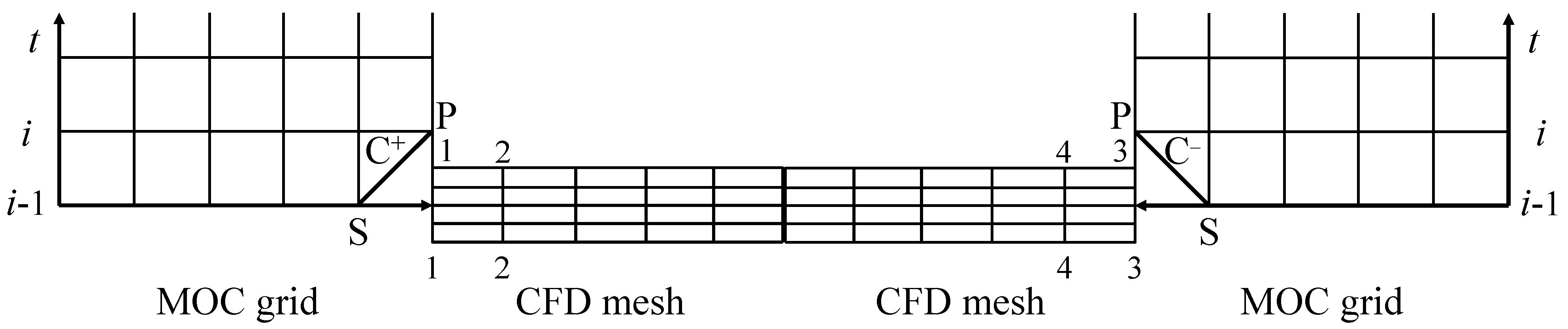
2.3. 1D–3D Coupling Interface

In this section, the basic coupling strategy follows the research of Wang [37], including the equations employed for solving the variables at the interface boundary and the distributions of the space and time steps. The numerical dilemma encountered and the improvements will be presented in Section 3.

For the coupling boundary, two equations are required to solve the velocity and pressure of the coupling boundary. The MOC part could provide a single characteristic equation for the coupling boundary, and another auxiliary equation is constructed from the CFD part, as shown in Figure 1.

In Figure 1, P represents the boundary node at the current time step, and S represents the neighbor node in the MOC part at the last time step. Cross-sections 1-1 and 2-2 surround all the cells next to the coupling interface in the CFD simulation region, as well as the cross-sections 3-3 and 4-4. The boundary conditions of CFD are set as a fixed uniform value, which assumes a constant spatial distribution at the coupling interface for the CFD part.

In the established model, the auxiliary equations still follow the research of Wang [37] based on Riemann invariants, given by:

$$H_P^i-\frac{a}{gA}{Q}_P^i=H_{P+1/2}^{i-1}-\frac{a}{gA}{Q}_{P+1/2}^{i-1}$$

(19)

$$H_P^i+\frac{a}{gA}{Q}_P^i=H_{P-1/2}^{i-1}+\frac{a}{gA}{Q}_{P-1/2}^{i-1}$$

(20)

Equations (19) and (20) are applied in Figure 1, respectively, where the subscript $1/2$ represents the variables defined as the volume average value of the cell centers adjacent to the interface. For example, $H_{P+1/2}$ in Equation (19) represents the volume average value of all cells located between cross-sections 1-1 and 2-2, and $H_{P-1/2}$ in Equation (20) represents the volume average value of all cells located between cross-sections 3-3 and 4-4. Cooperating Equations (19) and (20) with Equations (3) and (4), the four unknown variables at the two coupling interfaces could be determined by these four equations. The strategy of the coupling method could be summarized as follows:

1.

Carry out the 1D MOC part simulation;

2.

Carry out the 3D CFD part simulation;

3.

Derive the values of pressure and velocity at the coupling interface at the next time step by the variables at the current time step;

4.

Enter next time step.

The coupling method exhibited above could minimize the numerical disturbances and ensure no reflection is generated from the interface. The original coupling method in reference [37] employs a uniform space and time step length. The CFD and MOC program step forward with time synchronously. However, the consistent time and space steps have trouble when the pressure fluctuates rapidly. This numerical dilemma and corresponding solutions will be presented and discussed in detail in the next section.

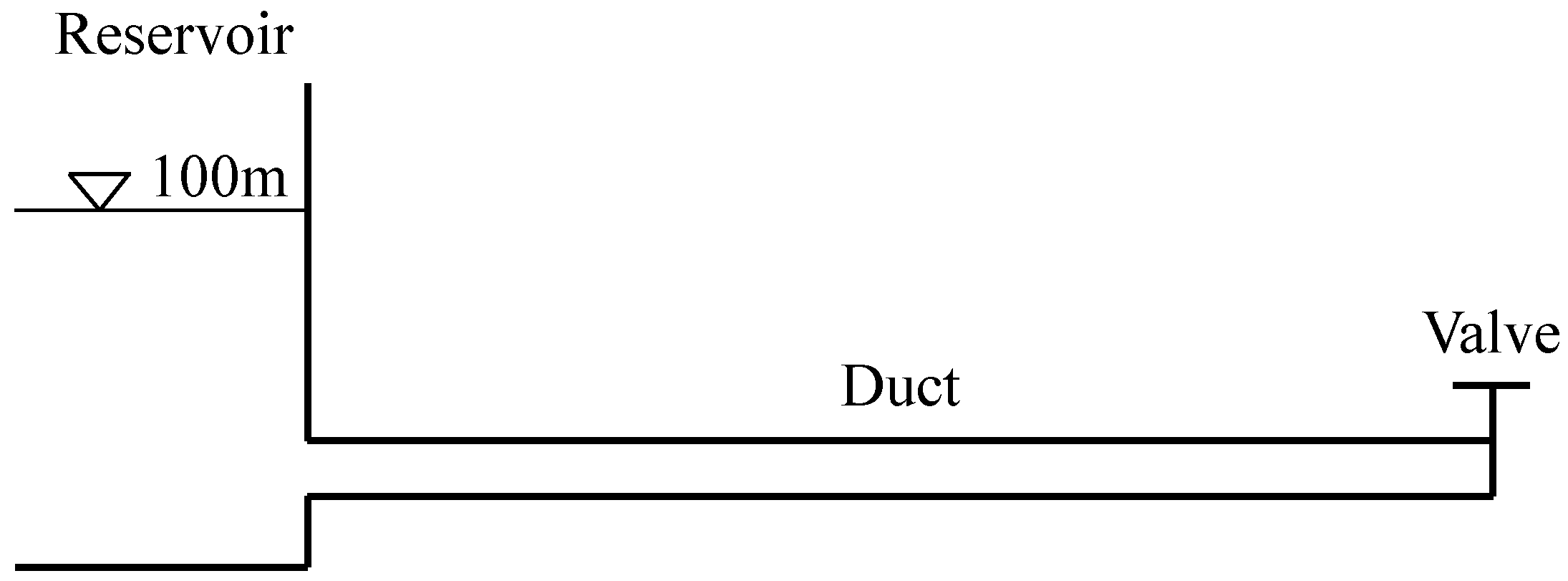
3. Validation of the Established Model

In this section, the established model is validated, including the ability of the 1D–3D coupling and the module of the mesh motion. The shortcomings of the CFD method are pointed out, and the solutions to remedy the numerical flaw are presented as well.

3.1. 1D–3D Coupling Validation

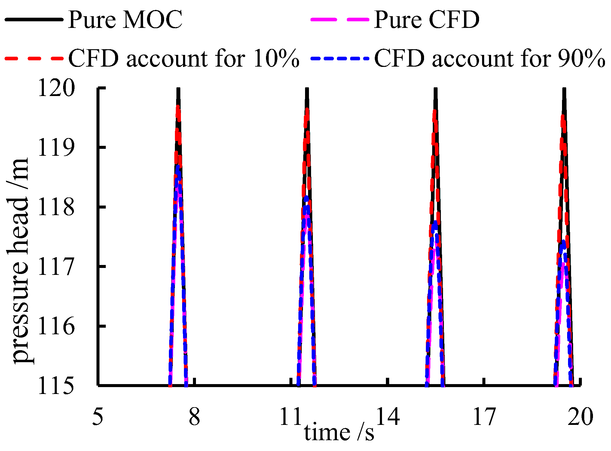
The strategy of the 1D–3D coupling is validated by a Reservoir–Duct–Valve System (RDVS), where linearly discharge and oscillating pressure variation boundary conditions are carried out at the valve, respectively. The schematic geometry of the system is shown in Figure 2.

As shown in Figure 2, the upstream of the square duct is a reservoir to provide the constant pressure head boundary. The downstream of the square duct connects a valve to control the discharge flow out of the duct. The cross-section area and length of the duct are 1 m² and 1000 m, respectively. The basic setup stays consistent with the reference [37]. The space and time steps are 5 m and 0.005 s, respectively. The water hammer velocity is 1000 m/s. The influence of the head loss is avoided by employing the slip wall boundary condition in CFD simulation and the zero head loss coefficient in the MOC part.

Four simulation configurations are compared to examine the 1D–3D coupling method, given by:

a.

Pure CFD.

b.

Pure MOC.

c.

The length of the CFD part takes 10% of the total length of the duct.

d.

The length of the CFD part takes 90% of the total length of the duct.

For configurations c and d, the CFD part is located at the center of the entire region, and the simulation region of the MOC is divided, on average, into two parts. In the CFD part, the advection terms are discretized by the upwind scheme; the interpolation of cell center to face center employs the linear scheme and the calculation of Laplacian and gradient terms; the discretization of time term employs the Crank–Nicolson scheme with the coefficient of 0.45.

3.1.1. Discharge Linearly Increases at the Valve

In the first situation, the discharge of the valve is set to linearly increase from 0 to 1 m³ in 5 s. The comparative results are exhibited in Figure 3.

It can be seen from Figure 3 that the results from different configurations are very similar and possess the same variation tendency. From a general view, Figure 3 indicates the 1D–3D coupling method performs well. However, the peak and valley values in Figure 3a slightly differ between various configurations. The zooming-up results of the red dotted box in Figure 3a are presented in Figure 4.

It can be seen from Figure 4 that the peak value decreases, with the CFD part occupying a greater proportion of the entire system. Additionally, the attenuation rate is faster than the MOC part. These tendencies and conclusions have also been reported in reference [37]. The main reason for the faster attenuation ratio and smoother peak values is that the time and space steps in the CFD part are not appropriate. In this simulated case, the ratios of space step and time step of both CFD and MOC are equal to the water hammer velocity. However, the pressure variation caused by the water hammer is much faster than the advection effect. In other words, for the CFD simulation, when the ratio of time step and space step is equal to the water hammer velocity, the pressure wave in the CFD may cross one cell in a single time step.

Therefore, the restriction on the discrete scales in space and time should guarantee the pressure wave cannot cross any cell. Similar to the Courant–Friedrichs–Lewy (CFL) condition, the following restriction should be theoretically satisfied in the CFD part:

$$\max \left(\frac{a\Delta t}{\Delta x}\right)<1$$

(21)

where $\Delta x$, $\Delta t$ are the space and time steps, respectively. However, the MOC method requires the value of $\frac{a\Delta t}{\Delta x}$ be strictly equal to one. Therefore, the uniform space and time steps of MOC and CFD are not suitable due to the paradoxical requirements.

According to Equation (21), the CFD part requires a minor time step to maintain the sharp peak and a lower attenuation rate to avoid the influence induced by the numerical flaw. The five kinds of time steps in pure CFD simulation are compared with pure MOC, as shown in Figure 5.

Figure 5 indicates that the performances are improved by decreasing the time step in the pure CFD method. There is still a particular gap between pure CFD and pure MOC results because the CFD method is not adapted to producing a high-pressure gradient unless an extremely tiny mesh size is employed. However, decreasing the mesh size may increase the computation requirement exponentially. Therefore, nonuniform space and time steps of MOC and CFD are recommended because elevating the precision by a minor time step is much more economical. Thus, the sharp pressure gradient could be preserved as much as possible.

In conclusion, the time steps of the MOC and CFD parts are consistent, and the space step in the CFD part should be several times that in the MOC part due to the restrictions of Equation (21) and the precondition in MOC.

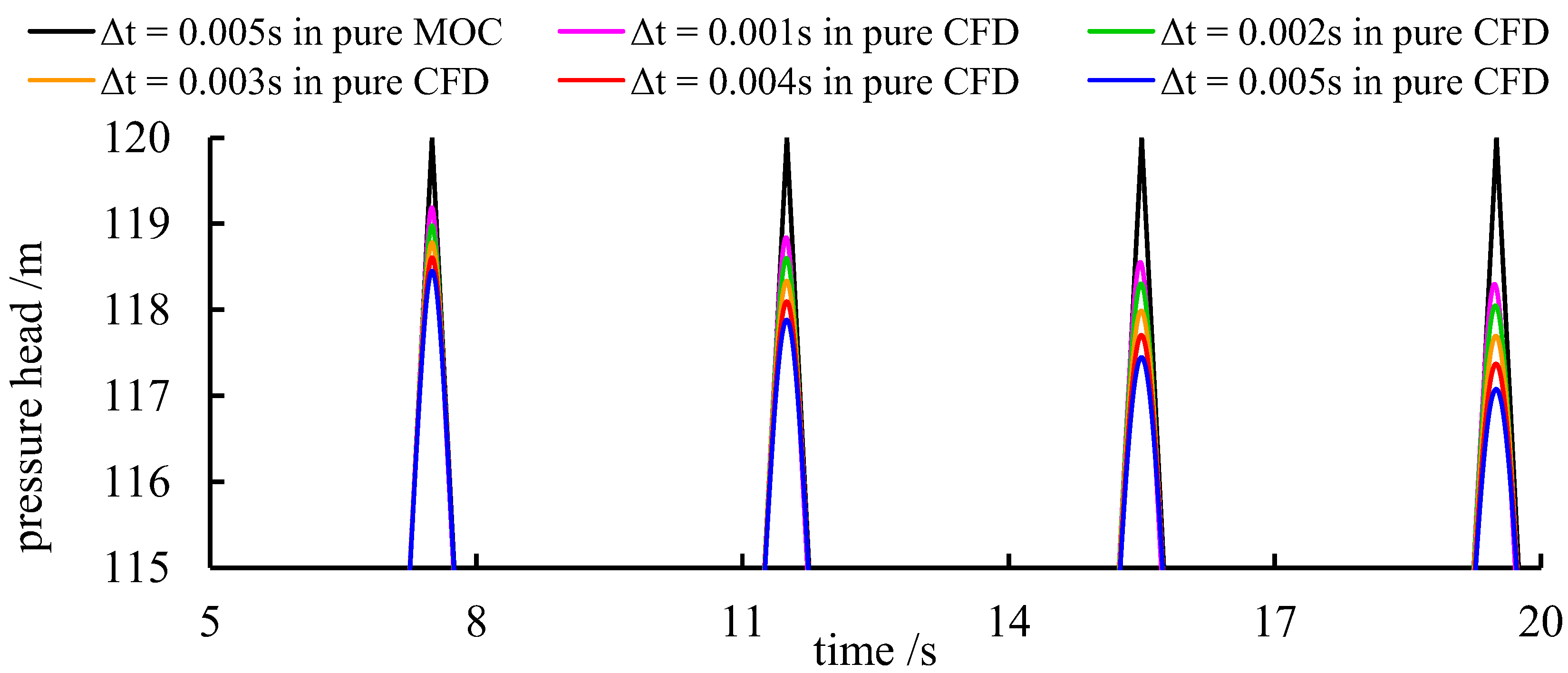
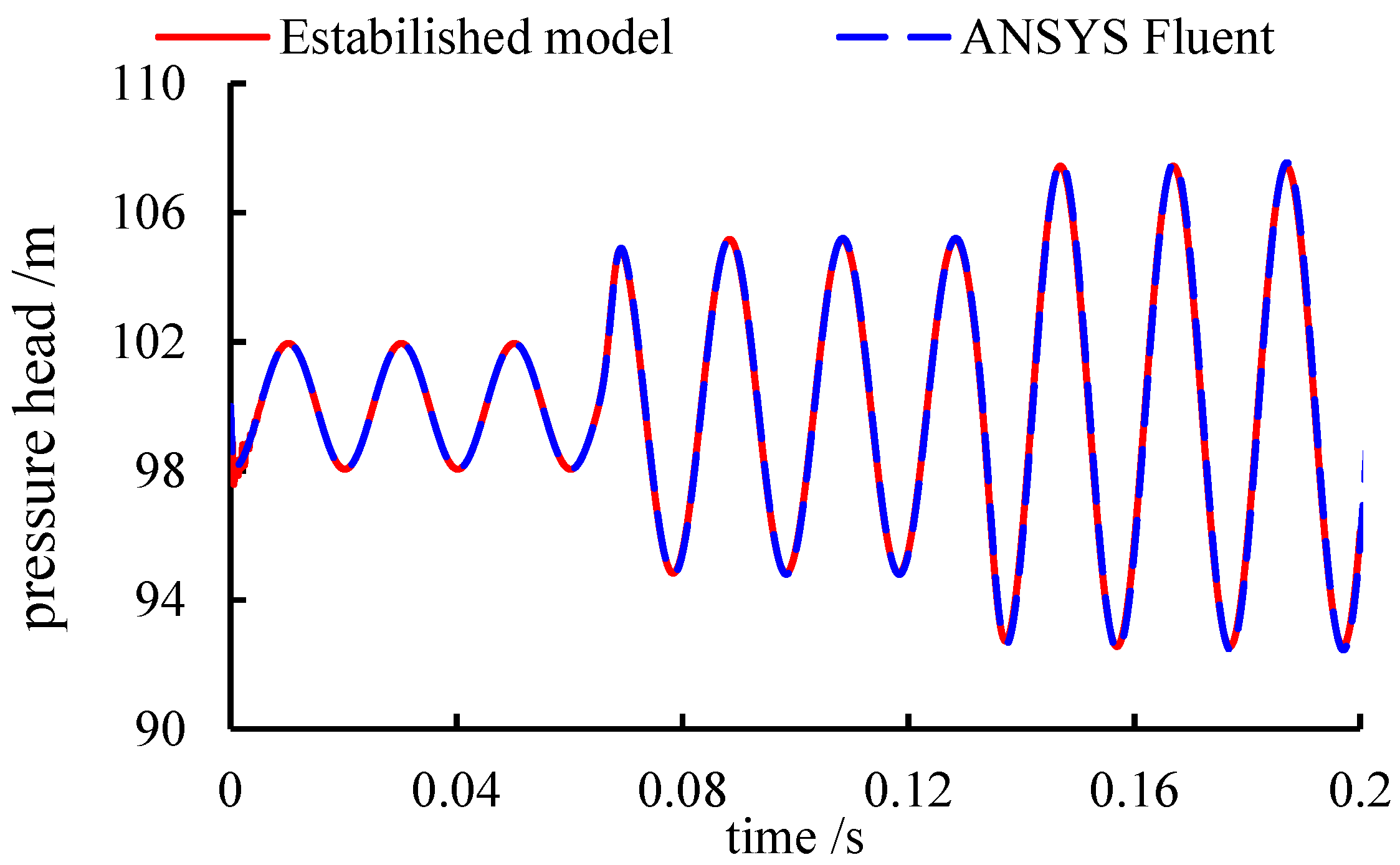
3.1.2. Pressure Oscillation at the Valve

The oscillating pressure at the value is employed to examine the ability of the coupling model. The same geometry shown in Figure 2 is used, and the pressure at the valve is set to be oscillating with constant magnitude and frequency.

The time steps of the CFD and MOC models are 2 × 10⁻⁵ s, and the space steps of the CFD and MOC models are 0.1 m and 0.02 m, respectively. The magnitude and frequency of the pressure oscillation at the valve are 1 m and 50 Hz, respectively. The results are shown in Figure 6.

It can be seen from Figure 6a that the results from different configurations are very close, and the peak value of the CFD dominating configuration is smaller than that of the MOC dominating configuration, as shown in Figure 6b.

The space steps and time steps are not uniform between CFD and MOC, and the value of $\max \left(\frac{a\Delta t}{\Delta x}\right)$ restricted in Equation (21) is equal to 0.2 in this section. Those setups could obtain a better result with lower computational resources required because further decreasing the mesh size in the CFD part will increase the computational resources exponentially.

Overall, Figure 6 indicates that the CFD-MOC coupling model could accurately predict the peak value and entire variation process under HFPF conditions when the MOC model accounts for most of the entire system. Therefore, the refined coupling strategy proposed in this study could be used to simulate the high-frequency forced vibration which frequently occurs in the hydraulic system.

3.2. Dynamic Mesh Validation

The mesh motion and corresponding mesh topology change are considered in the established model to generate a numerical vibration source in the hydraulic system. In this study, the pipe vibration is employed to induce a pressure oscillation. The validation of the mesh motion is implemented by comparing the results of pressure oscillation obtained by the established model with the commercial software ANSYS Fluent. The geometry of the pipe vibration case is presented in Figure 7.

Figure 7 presents a Reservoir–Duct–Reservoir system (RDRS). As shown in Figure 7, a square duct is located between two reservoirs, and the center of the duct is vibrating in a manner of constant frequency and amplitude. The water in the vibration region is compressed under the effect of the wall oscillation, and a pressure oscillation is thus produced with the same frequency as the wall oscillation. The pipe vibration could be used to analyze the forced vibration in the hydraulic system, which could not be derived by the 1D method. In the 3D CFD method, the pipe vibration could be simulated by the dynamic mesh method, and then a perfect vibration source is numerically generated.

The correctness of the modeling of mesh motion in the established is validated by comparing the variation and magnitude of the pressure oscillation obtained by ANSYS Fluent. The displacement of the pipe walls satisfies $s=T\sin \left(2\pi ft\right)$, where $T$, $f$ are the vibration magnitude and frequency, respectively. Figure 8 gives the comparative results between the established model and ANSYS Fluent.

It can be seen from Figure 8 that the various processes and peak values of the pressure agree well with each other, which demonstrates the correctness of the dynamic mesh module implanted in the established model. The propagation of the water hammer is much quicker than the advection flow. Therefore, the influence of most discretization schemes on the results is insignificant, including the discretization schemes of the advection and the transient terms.

The initial states of pressure variations presented in Figure 8 are rapidly fluctuating due to the moving velocity of the wall reaching its maximum at $t=0$. The fluid at the initial state is rapidly compressed and induces a chaotic pressure perturbation. The pressure variation at the center of the system is superimposed by the reflected wave of the water hammer after $t=0.067\mathrm{s}$. The detailed superimposed effect will be discussed in the next section.

Furthermore, the magnitudes of the pressure oscillation under various vibration frequencies and amplitudes of the walls are compared, as shown in Figure 9.

It could be seen from Figure 9 that the amplitude of the pressure oscillation obtained by the established model is quite similar to the results of ANSYS Fluent; the difference is less than 0.1%. The results shown in Figure 8 and Figure 9 demonstrate the correctness of the dynamic mesh module in the established model.

Overall, combined with the analysis in Section 3.1, the results indicate that the established model is suitable for analyzing the HFPF in the hydraulic system.

4. Forced Vibration Analysis

In this section, the dynamic processes of the HFPF are simulated and analyzed based on the 1D–3D coupling method. It should be mentioned that the forced vibration source cannot be achieved directly by the 1D method. Therefore, the numerical vibration source is generated in the CFD part by forcing the walls of the pipe to vibrate. Additionally, the dynamic mesh method in the CFD model is employed to realize the displacement of the pipe walls.

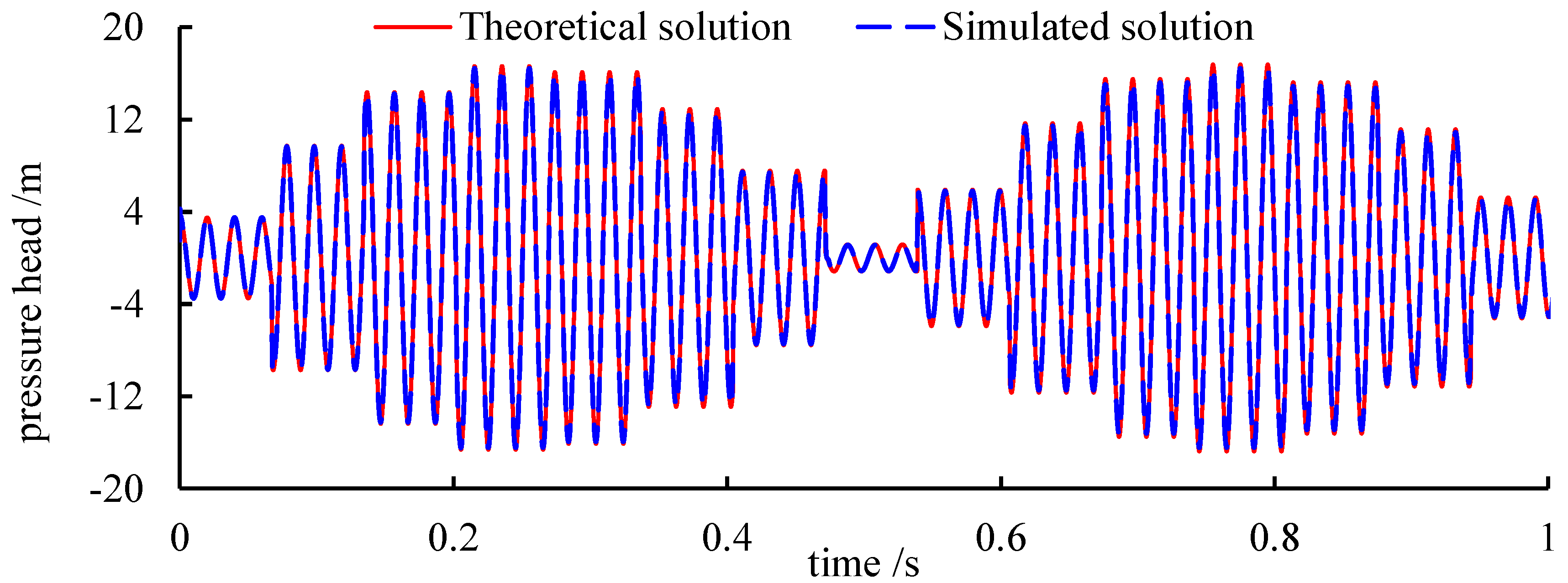
4.1. Pressure Oscillation Induced by Wall Vibration

The same geometry as in Section 3.2 is used to analyze the propagation and superposition characteristics of the high-frequency forced vibration in a simple hydraulic system consisting of two reservoirs and one square pipe. The vibration range and the magnitude of the pipe vibration are set as 0.1 m and 200 μm, respectively, to avoid the influence of the face vibration source. The 1D–3D coupling method, where the 3D part accounts for 4% of the entire system, is employed for computation-consuming consideration and to minimize the numerical attenuation in the CFD part. The time and space steps remain consistent with Section 3.1.2. The pressure variation at the center of the system is given in Figure 10, as follows.

It can be seen from Figure 10 that the amplitudes of pressure oscillation are not constant, and have been enlarged several times compared with that at the initial state. Generally, this enlarging phenomenon is caused by the superimposition effect of the reflected wave from the reservoir boundaries. The process of the pressure variation could be derived from the superposition principle of a pressure wave with the following hypothesis:

Hypothesis 1.

For HFPF, the influence of the advection effect is neglectable compared with the propagation of the water hammer.

Hypothesis 2.

Pressure waves from various sources satisfy the independence principle.

For Hypothesis 1, the velocity of the fluid is far less than the water hammer velocity; therefore, the advection effect could be neglected, and the analysis of the pressure oscillation could ignore the influence of discharge oscillation. Hypothesis 2 is the commonly used assumption when analyzing the vibration and wave. For the pressure wave driven by the water hammer, any single pressure wave can be decomposed into two sub-waves. In the same way, two pressure waves can be combined to form a new pressure wave. Therefore, Hypothesis 2 is also reasonable.

Assuming point B is the vibration source and generates steady pressure oscillation, which satisfies $P_m\sin \left(\omega t+\phi \right)$, Points A and C are reservoirs. The distance from point B to the reservoir boundary is $L$; thus, the pressure wave takes the time $L/a$ to reach the boundary. Therefore, when the pressure wave arrives, the expression of which can be written as $P_m\sin \left[\omega \left(t-\frac{L}{a}\right)+\phi \right]$.

For the reservoir boundary with a constant pressure boundary condition, the reflected wave has the same oscillation magnitude, but the phase difference is $\pi$. Consequently, the sum of incident and reflected waves is equal to zero. Subsequently, the reflected wave takes another $2L/a$ to reach point B. Therefore, the reflected wave at point B is $P_m\sin \left[\omega \left(t-\frac{2L}{a}\right)+\phi -\pi \right]$, and the total pressure of point B is $P_m\sin \omega t+P_m\sin \left[\omega \left(t-\frac{2L}{a}\right)+\phi -\pi \right]$.

Similarly, if the pressure wave generated at point B spreads to both sides, the total pressure of point B when both of the reflected waves arrive at point B is $P_m\sin \omega t+P_m\sin \left[\omega \left(t-\frac{2L_1}{a}\right)+\phi -\pi \right]+P_m\sin \left[\omega \left(t-\frac{2L_2}{a}\right)+\phi -\pi \right]$, where $L_1$, $L_2$ are the distances from point B to the reservoirs of both sides, respectively. The magnitude of the source pressure oscillation induced by pipe vibration can be estimated by [18]:

$$p_m=\frac{\left(A-A^{\prime }\right)\omega L}{2aA}K$$

(22)

where $A$ is the cross-sectional area of the pipe; $A^{\prime }$ is the minimum cross-sectional area during the pipe vibration; $\omega$, $L$ are the angular vibration frequency and the length of the vibration region, respectively; $K$ is the bulk modulus of the fluid in the pipe.

The integrated propagation process can be described in Figure 11.

The blue and red dashed lines in Figure 11 represent the traveling waves spreading to the left and right sides at the beginning. The time of the traveling wave spends reaching the reservoir boundary is marked on the left and right sides in Figure 11. The solid points represent the reflected waves that arrive at point B, and the expressions of the reflected waves are given nearby. The traveling waves are mapped to the time axis to obtain the time coordinates. It should be noted that the blue and red lines intersect with the black dashed line at the marked point in Figure 11, which means both the traveling waves cross the distance of $2L_1+2L_2$ at time $t=\frac{2L_1+2L_2}{a}$.

The superimposed pressure oscillation at any location in the pipeline can be derived by summing all the solid points in the graphic within a specific time. For example, the pressure oscillation at point B in Figure 11 can be described as a piecewise function:

$$P_B=\left\{\begin{array}{cc}{P}_0\hfill & \hfill t<\frac{2L_1}{a}\\ P_0+P_1\hfill & \hfill \frac{2L_1}{a}\le t<\frac{2L_2}{a}\\ P_0+P_1+P_2\hfill & \hfill \frac{2L_2}{a}\le t<\frac{2L_1+2L_2}{a}\\ P_0+P_1+P_2+2P_3\hfill & \hfill \frac{2L_1+2L_2}{a}\le t<\frac{4L_1+2L_2}{a}\\ & \dots \hfill \end{array}\right.$$

(23)

where $P_0=P_m\sin \left(\omega t+\phi \right)$, $P_1=P_m\sin \left[\omega \left(t-\frac{2L_1}{a}\right)+\phi -\pi \right]$, $P_2=P_m\sin \left[\omega \left(t-\frac{2L_1}{a}\right)+\phi -\pi \right]$, $P_3=P_m\sin \left[\omega \left(t-\frac{2L_1+2L_2}{a}\right)+\phi -2\pi \right]$.

To validate the correctness of Equation (23), comparison of the results in Figure 10 and Equation (23) is shown in Figure 12.

The magnitude and phase lag of the initial pressure oscillation in the theoretical solution is obtained from the simulated solution and given by $P_m=3.5 \mathrm{m}$ and $\phi =-4.74\mathrm{rad}$, respectively. It can be seen from Figure 12 that the dynamic process of pressure variation derived by the theoretical and simulated solutions agree well with each other, which validates Equation (23) and the theoretical analysis in Figure 11.

Furthermore, Figure 12 also demonstrates the independence principle of the HFPF in the hydraulic system, which is employed in this section as Hypothesis 2. According to the independence principle of pressure fluctuation, multi-frequency pressure oscillation can be superimposed to analyze and evaluate the overall performance of the entire system.

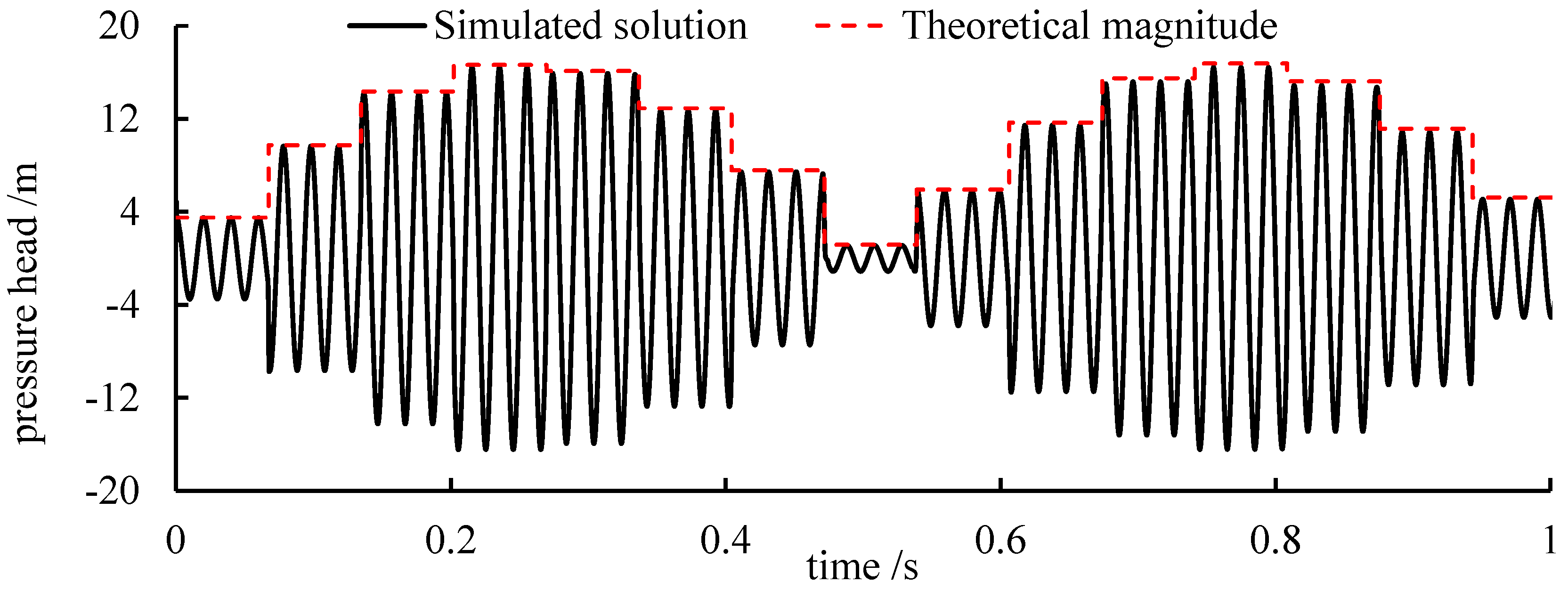
4.2. Magnitude of the Pressure Fluctuation

Figure 10 and Figure 12 show varying oscillation magnitude of the pressure fluctuation due to the superposition of the reflected pressure wave. Therefore, the variation in the pressure oscillation should be considered for the safety of the engineering design, which will be analyzed as follows.

For the same pressure oscillation source presented in Figure 11, the time-domain expression at the initial state can be given by:

$$P_{B,0}=P_{m,0}\sin \left(\omega t+{\phi }_0\right)$$

(24)

where, $P_{m,0}$, ${\phi }_0$ are the magnitude and phase angle at the beginning; $P_B{}_{,0}$ is the pressure at point B in the initial state. When the first reflected pressure wave arrives at point B, the superimposed pressure of point B can be written as:

$$P_{B,1}=P_{B,0}+P_{m,0}\sin \left[\omega \left(t-\frac{2L}{a}\right)+{\phi }_0-\pi \right]$$

(25)

Equation (25) can be simplified by basic trigonometric formulas:

$$P_{B,1}=P_{m,1}\sin \left(\omega t+{\phi }_1\right)$$

(26)

where $P_{m,1}=P_{m,0}\sqrt{2-2\cos \frac{2\omega L}{a}}$, ${\phi }_1=\arctan \left[\frac{\sin {\phi }_0+\sin \left(\frac{2\omega L}{a}-{\phi }_0\right)}{\cos {\phi }_0-\cos \left(\frac{2\omega L}{a}-{\phi }_0\right)}\right]-\pi$.

It can be seen from Equation (26) that the primary form of the superimposed pressure expression is similar to the original expression. The magnitude and phase angle can both be determined by the values from the last superimposition. The general form of the superimposed pressure expression can be written as:

$$P_{B,i}=P_{m,i}\sin \left(\omega t+{\phi }_i\right)$$

(27)

The amplitude and phase angle are given by:

$$P_{m,i}=\sqrt{P_{m,i-1}^2+P_{m,0}^2+2P_{m,i-1}{P}_{m,0}\cos \left({\phi }_{i-1}-{\psi }_i\right)}$$

(28)

$${\phi }_i=\left\{\begin{array}{cc}\arctan \frac{B}{A}\hfill & \hfill A>0\\ \arctan \frac{B}{A}+\pi \hfill & \hfill A<0,B\ge 0\\ \arctan \frac{-B}{-A}+\pi \hfill & \hfill A<0,B<0\end{array}\right.$$

(29)

where $A=P_{m,i-1}\cos {\phi }_{i-1}+P_{m,0}\cos {\psi }_i$, $B=P_{m,i-1}\sin {\phi }_{i-1}+P_{m,0}\sin {\psi }_i$; subscripts $i$ and $i-1$ represent the value after and before the superposition of the reflected wave; ${\psi }_i$ represents the phase angle of the traveling wave arriving at point B. The value of ${\psi }_i$ can be directly obtained from Figure 11, where the expressions of the traveling wave have been marked.

Once the system is determined, using Equations (24)–(29) can directly derive the magnitudes of the pressure oscillation at any state. For the results presented in Figure 10, the magnitude of the pressure oscillation at any state can be derived using Equations (24)–(29), as shown in Figure 13.

Figure 13 shows the theoretical magnitude of the pressure oscillation presented in Figure 10 by Equations (24)–(29). It can be seen that the magnitude is ideally predicated, which demonstrates the deductive process of the vibration magnitude in this section.

It should be noted that the predicating magnitude and the time-domain variation process of the pressure oscillation are suitable for any location in the pipeline. Additionally, for other complicated layouts of the hydraulic systems, the theories in this section are still suitable with the reconsideration of the boundary conditions.

5. Conclusions

This study established a 1D–3D coupling model with mesh motion and mesh topology change implanted. The numerical flaws in the CFD model for HFPV were discussed. The high-frequency vibration source was numerically generated in a hydraulic system by the pipe vibration. The superposition principle of the pressure fluctuation was demonstrated, and the theoretical variation and magnitude of the pressure oscillation were derived. The established 1D–3D coupling model and theoretical analysis method could be referenced by other complex hydraulic systems. The main conclusions are as follows.

(1)

The established 1D–3D coupling model could comparably precisely simulate the dynamic process of the pressure oscillation and propagation in the pipe system, overcoming the overdetermined problem in the traditional 1D method. The established model is applicable to forced vibration analysis in the hydraulic system.

(2)

The magnitude of the original pressure oscillation could be enlarged several times by the reflected waves. Additionally, the coupling method of 1D–3D could accurately consider the influence of the reflected waves with comparatively low computational resources required.

(3)

The pressure oscillation in the hydraulic system satisfies the independence principle. Additionally, the exhibit pressure fluctuation is the multiple superpositions of the traveling and the standing waves.

The established 1D–3D coupling model and the theoretical analysis of the HFPF could be consulted for further research on complex layouts of the hydraulic facilities. This paper focused on the fundamental study of the forced vibration and the mechanism of the superposition phenomenon of the sonic pressure wave propagations, the coupling with other complicated hydraulic structures could be further investigated, e.g., surge tank, hydraulic turbine, etc.

References

1. Favrel, A.; Müller, A.; Landry, C.; Yamamoto, K.; Avellan, F. Study of the vortex-induced pressure excitation source in a Francis turbine draft tube by particle image velocimetry. Exp. Fluids 2015, 56, 215. [Google Scholar] [CrossRef]
2. Trivedia, C.; Gandhi, B.K.; Cervantes, M.J.; Dahlhaug, O.G. Experimental investigations of a model Francis turbine during shutdown at synchronous speed. Renew. Energy 2015, 83, 828–836. [Google Scholar] [CrossRef]
3. Qian, Z.D.; Yang, J.D.; Huai, W.X. Numerical simulation and analysis of pressure pulsation in Francis hydraulic turbine with air admission. J. Hydrodyn. 2007, 19, 467–472. [Google Scholar] [CrossRef]
4. Gao, Y.; Zhang, Q.; Kong, X. Wavelet-based pressure analysis for hydraulic pump health diagnosis. Trans. ASAE 2003, 46, 969–976. [Google Scholar]
5. Yang, Y.; Zhou, L.; Shi, W.D.; He, Z.; Han, Y.; Xiao, Y. Interstage difference of pressure pulsation in a three-stage electrical submersible pump. J. Pet. Sci. Eng. 2021, 196, 107653. [Google Scholar] [CrossRef]
6. Yang, S.S.; Kong, F.Y.; Qu, X.Y.; Jiang, W.-M. Influence of blade number on the performance and pressure pulsations in a pump used as a turbine. J. Fluids Eng.-Trans. ASME 2012, 134, 124503. [Google Scholar] [CrossRef]
7. Kirschner, O.; Ruprecht, A.; Gode, E.; Riedelbauch, S. Experimental Investigation of Pressure Fluctuations Caused by a Vortex Rope in a Draft Tube. In Proceedings of the 26th IAHR Symposium on Hydraulic Machinery and Systems, Tsinghua University, Beijing, China, 19–23 August 2012. [Google Scholar]
8. Valentín, D.; Presas, A.; Egusquiza, E.; Valero, C.; Egusquiza, M.; Bossio, M. Power swing generated in Francis turbines by part load and overload instabilities. Energies 2017, 10, 2124. [Google Scholar] [CrossRef] [Green Version]
9. Hasmatuchi, V.; Farhat, M.; Roth, S.; Botero, F.; Avellan, F. Experimental evidence of rotating stall in a pump-turbine at off-design conditions in generating mode. J. Fluids Eng.-Trans. ASME 2011, 133, 051104. [Google Scholar] [CrossRef]
10. Zhang, X.X.; Cheng, Y.G.; Xia, L.S.; Yang, J.D.; Qian, Z.D. Looping dynamic characteristics of a pump-turbine in the s-shaped region during runaway. J. Fluids Eng.-Trans. ASME 2016, 138, 091102. [Google Scholar] [CrossRef]
11. Zhou, J.X.; Cai, F.L.; Wang, Y. New elastic model of pipe flow for stability analysis of the governor-turbine-hydraulic system. J. Hydraul. Eng.-ASCE 2011, 137, 1238–1247. [Google Scholar] [CrossRef]
12. Suo, L.S.; Wylie, E.B. Impulse response method for frequency-dependent pipeline transients. J. Hydraul. Eng. 1989, 111, 478–483. [Google Scholar] [CrossRef]
13. Suo, L.S.; Wylie, E.B. Hydraulic transients in rock-bored tunnels. J. Hydraul. Eng. 1990, 116, 196–210. [Google Scholar] [CrossRef]
14. Ruchonnet, N. Multiscale Computational Methodology Applied to Hydroacoustic Resonance in Cavitating Pipe Flow. Ph.D. Thesis, Swiss federal Institute of Technology in Lausanne, Lausanne, Switzerland, 2010. [Google Scholar]
15. Wylie, E.B.; Streeter, V.L.; Suo, L.S. Fluid Transients in Systems; Prentice-Hall: New York, NY, USA, 1993. [Google Scholar]
16. Morris, D. Linear Control Systems Engineering; Tsinghua University Press: Beijing, China, 2005. [Google Scholar]
17. Yan, W.J.; Yang, J.B.; Zhao, Z.G.; Yang, J.D.; Yang, W.J. Global matrix method for frequency-domain stability analysis of hydropower generating system. J. Clean. Prod. 2022, 333, 130097. [Google Scholar] [CrossRef]
18. Yang, X.W.; Lian, J.J.; Wang, H.J.; Luo, L.W. Study on the forced vibration induced by the high-frequency pipe vibration. J. Hydroelectr. Eng. 2022, 6, 102–111. [Google Scholar]
19. Zhou, J.X. Vibration Characteristics and Stability Analysis of Hydropower Station with Long Water Conveyance System; China Water & Power Press: Beijing, China, 2011. (In Chinese) [Google Scholar]
20. Orczyk, J.J.; Barczak, A.; Costa-Faidella, J.; Kajikawa, Y. Cross laminar traveling components of field potentials due to volume conduction of non-traveling neuronal activity in macaque sensory cortices. J. Neurosci. 2021, 41, 7578–7590. [Google Scholar] [CrossRef]
21. Sturzebecher, D.; Nitsche, W. Active cancellation of tollmien-schlichting instabilities on a wing using multi-channel sensor actuator systems. Int. J. Heat Fluid Flow 2003, 24, 572–583. [Google Scholar] [CrossRef]
22. Li, Y.B.; Ren, Y.K.; Liu, W.Y.; Chen, X.M.; Tao, Y.; Jiang, H.Y. On controlling the flow behavior driven by induction electrohydrodynamics in microfluidic channels. Electrophoresis 2017, 38, 983–995. [Google Scholar] [CrossRef]
23. Semerci, D.S.; Yavuz, T.I. Increasing Efficiency of an Existing Francis Turbine by Rehabilitation Process. In Proceedings of the 5th IEEE International Conference on Renewable Energy Research and Applications (ICRERA), Birmingham, UK, 20–23 November 2016. [Google Scholar]
24. Tiwari, G.; Kumar, J.; Prasad, V.; Patel, V.K. Utility of CFD in the design and performance analysis of hydraulic turbines—A review. Energy Rep. 2020, 6, 2410–2429. [Google Scholar] [CrossRef]
25. Oh, H.W.; Yoon, E.S. Application of computational fluid dynamics to performance analysis of a francis hydraulic turbine. Proc. Inst. Mech. Eng. Part A 2007, 221, 583–590. [Google Scholar] [CrossRef]
26. Fu, X.L.; Li, D.Y.; Wang, H.J.; Li, Z.G.; Zhao, Q.; Wei, X.Z. One- and three-dimensional coupling flow simulations of pumped-storage power stations with complex long-distance water conveyance pipeline system. J. Clean. Prod. 2021, 315, 128228. [Google Scholar] [CrossRef]
27. Kong, K.J.; Jung, S.H.; Jeong, T.Y.; Koh, D.K. 1D-3D coupling algorithm for unsteady gas flow analysis in pipe systems. J. Mech. Sci. Technol. 2019, 33, 4521–4528. [Google Scholar] [CrossRef]
28. Liu, D.M.; Zhang, X.X.; Yang, Z.Y.; Liu, K.; Cheng, Y.G. Evaluating the pressure fluctuations during load rejection of two pump-turbines in a prototype pumped-storage system by using 1d-3d coupled simulation. Renew. Energy 2021, 171, 1276–1289. [Google Scholar] [CrossRef]
29. Toti, A.; Vierendeels, J.; Belloni, F. Coupled system thermal-hydraulic/CFD analysis of a protected loss of flow transient in the MYRRHA reactor. Ann. Nucl. Energy 2018, 118, 199–211. [Google Scholar] [CrossRef]
30. Zhang, H.; Guo, J.; Lu, J.; Niu, J.; Li, F.; Xu, Y. The comparison between nonlinear and linear preconditioning JFNK method for transient neutronics/thermal-hydraulics coupling problem. Ann. Nucl. Energy 2019, 132, 257–368. [Google Scholar] [CrossRef]
31. Gui, X.; Wong, L.N.Y. A 3D fully thermo–hydro–mechanical coupling model for saturated poroelastic medium. Comput. Methods Appl. Mech. Eng. 2022, 394, 114939. [Google Scholar]
32. Yang, S.; Chen, X.; Wu, D.Z.; Yan, P. Dynamic analysis of the pump system based on MOC-CFD coupled method. Ann. Nucl. Energy 2015, 78, 60–69. [Google Scholar] [CrossRef]
33. Wu, D.Z.; Yang, S.; Wu, P.; Wang, L. MOC-CFD coupled approach for the analysis of the fluid dynamic interaction between water hammer and pump. J. Hydraul. Eng. 2015, 141, 06015003. [Google Scholar] [CrossRef]
34. Ruprecht, A.; Helmrich, T.; Aschenbrennert, T.; Scherer, T. Simulation of vortex rope in a turbine draft tube. In Proceedings of the 21st IAHR Symposium on Hydraulic Machinery and Systems, Lausanne, Switzerland, 9–12 September 2002. [Google Scholar]
35. Ruprecht, A.; Helmrich, T. Simulation of the water hammer in a hydro power plant caused by draft tube surge. In Proceedings of the 4th ASME/JSME Joint Fluids Engineering Conference, Honolulu, HI, USA, 6–10 July 2003. [Google Scholar]
36. Zhang, X.X.; Cheng, Y.G. Simulation of hydraulic transients in hydropower systems using the 1-D–3-D coupling approach. J. Hydrodyn. 2012, 24, 595–604. [Google Scholar] [CrossRef]
37. Wang, C.; Nilsson, H.; Yang, J.D.; Petit, O. 1D–3D coupling for hydraulic system transient simulations. Comput. Phys. Commun. 2017, 210, 1–9. [Google Scholar] [CrossRef]
38. Politano, M.; Odgaard, A.J.; Klecan, W. Case study: Numerical evaluation of hydraulic transients in a combined sewer overflow tunnel system. J. Hydraul. Eng. 2007, 133, 1103–1110. [Google Scholar] [CrossRef]
39. Jasak, H. Error Analysis and Estimation for the Finite Volume Method with Applications to Fluid Flows. Ph.D. Thesis, Imperial College London, London, UK, 1996. [Google Scholar]
40. Moukalled, F.; Mangani, L.; Darwish, M. The Finite Volume Method in Computational Fluid; Springer: Cham, Switzerland, 2016. [Google Scholar]
41. Ansys Inc. Ansys Fluent User’s Guide; Ansys Inc.: Canonsburg, PA, USA, 2020. [Google Scholar]
42. Open FOAM Foundation Ltd. Open FOAM User Guide; Open FOAM Foundation Ltd.: London, UK, 2020. [Google Scholar]
43. Ansys Inc. Ansys Fluent Theory Guide; Ansys Inc.: Canonsburg, PA, USA, 2020. [Google Scholar]
Figure 1. Schematic diagram of the 1D–3D coupling.
Energies 15 06051 g001
Figure 2. Schematic geometry of the RDVS.
Energies 15 06051 g002
Figure 3. Pressure variation when the discharge at the valve linearly increases. (a) Pressure head at the center of the entire system (b) pressure head at the valve.
Energies 15 06051 g003
Figure 4. Peak value of the pressure head at the center of the entire system.
Energies 15 06051 g004
Figure 5. Peak value of the pressure head under various time step sizes.
Energies 15 06051 g005
Figure 6. Pressure head variation at the center of the entire system. (a) Overview (b) zoom-up view.
Energies 15 06051 g006
Figure 7. Schematic geometry of the vibration pipe.
Energies 15 06051 g007
Figure 8. Pressure variation at the center of the vibration region ( T = 20   μ m , f = 50   Hz ).
Energies 15 06051 g008
Figure 9. Magnitude of the pressure oscillation. (a) Vibration frequency (b) vibration magnitude.
Energies 15 06051 g009
Figure 10. Pressure variation at the center of the system.
Energies 15 06051 g010
Figure 11. Graphical method of the traveling waves.
Energies 15 06051 g011
Figure 12. Comparative results of the pressure oscillation.
Energies 15 06051 g012
Figure 13. Theoretical magnitude of the pressure oscillation.
Energies 15 06051 g013
Publisher’s Note: MDPI stays neutral with regard to jurisdictional claims in published maps and institutional affiliations.