Impact of Passive-Components’ Models on the Stability Assessment of Inverter-Dominated Power Grids

Abstract

Power systems are experiencing some profound changes, which are posing new challenges in many different ways. One of the most significant of such challenges is the increasing presence of inverter-based resources (ibrs), both as loads and generators. This calls for new approaches and a wide reconsideration of the most commonly established practices in almost all the levels of power systems’ analysis, operation, and planning. This paper focuses specifically on the impacts on stability analyses of the numerical models of power system passive components (e.g., lines, transformers, along with their on-load tap changers). Traditionally, loads have been modelled as constant power loads, being this both a conservative option for what concerns stability results and a computationally convenient simplification. However, compared to their counterparts above, in some operating conditions ibrs can effectively be considered real constant power loads, whose behaviour is much more complex in terms of the equivalent impedance seen by the network. This has an impact on the way passive network components should be modelled to attain results and conclusions consistent with the real power system behaviour. In this paper, we investigate these issues on the ieee14 bus test network. To begin with, we assess the effects of constant-power and constant-impedance load models. Then, we replace a transmission line with a dc line connected to the network through two modular multilevel converters (mmcs), which account for the presence of ibrs in modern grids. Lastly, we analyse how and to which extent inaccurate modelling of mmcs and other passive components can lead to wrong stability analyses and transient simulations.

1. Introduction

During this last decade, power electronics converters have been integrated at an ever-rising pace in generation, transmission, and distribution power systems. This technology lends itself to a plethora of applications: among others, it could be used as a grid interface for specific kinds of loads (i.e., converter-connected loads (ccls)) or as a means for energy conversion in generation systems fed by fuel cells or renewable energy sources, such as wind or solar photovoltaic (i.e., converter-interfaced generation (cig)). Both usages can be grouped into the broad class of inverter-based resources (ibrs).

The increasing presence of ibrs has numerous ramifications in different facets of modern electric power systems, such as planning and operation. According to [1], ibrs are significantly changing power system dynamic behaviour (and, most notably, oscillatory behaviour during disturbances [2]) to the extent that the basic stability terms developed in the literature have been recently revised to consider the fast response of converters. Moreover, due to the progressive phase-out of conventional synchronous generators, cig is expected to have a prominent role in supporting the stability of future grids through the provision of specific services, namely frequency and voltage regulation. In the light of the above, the interactions of ibrs with the power grid must be accurately studied to ensure a correct operation at all times.

Before the arrival of ibrs, conventional generation and transmission systems were typically simulated through single-phase equivalent representations and static load and transformer models. This modelling approach was originally imposed during the development of the first power system simulators to overcome the deficiency in the capability of computational systems to perform calculations using detailed, dynamic three-phase models. Based on this simulation setting, generator, transformer, line, and load models have been developed over the years to accurately simulate and predict the complex behaviour of electricity grids. In particular, some models have become customarily based on particular assumptions that were true in the past. For instance, a widely adopted approach is to describe lines with algebraic (i.e., static) representations and loads with constant power models to perform simulations of worst-case scenarios. As shown by the results of a survey collected in [3], about 70% of utilities and system operators in the world adopt only static load models for steady-state power system studies. The only exception is represented by utilities and system operators in the USA, which use a combination of static and dynamic models. In addition to this, static load models are typically set as constant power loads, and distributed generation is modelled as negative loads. This modelling approach is also dominant when it comes to dynamic power system analyses. Although the survey dates back to 2010, this practice does not seem to have changed up to at least 2018 and 2022, when [4,5], which also deal with the topic of load modelling, were respectively published. In [4] the typical values for the static models under different operating conditions are described. In [5] the impact of two static load models (i.e, exponential and polynomial model) on small-signal, transient, and frequency stability studies has been assessed. The conclusion of this work is that, in case no accurate data on loads are available, a constant power model should be adopted, as it provides the worst-case scenario and therefore constitutes a conservative approach. This same point is raised in [6,7]. Another practice established in power system analysis to typically accelerate simulations is to adopt static line models instead of dynamic ones [8,9].

In this article, we want to highlight how these approaches should be used with care in the case of ibr-dominated grids, as they might lead to a misguided power system stability assessment. Indeed, the growing presence of ibrs is significantly changing the behaviour of electric power systems. This begs the question as to whether previously developed load and passive elements models (and the assumptions in which they ground) are still adequate in the presence of ibr-dominated power grids or require revision—a question this paper attempts to answer. This is the same question the authors of [10] pose in the conclusion of their work. After describing the challenges ibrs bring to power systems stability studies, they suggest that the increasing penetration of ibrs may produce new ways through which instability occurs, calling for both more accurate models and new simulation techniques. In particular, the work presented here delves into the most commonly adopted models of loads and passive elements (i.e., lines, transformers, and shunts). After elaborating on their usage in conventional power systems, we assess how these models could be modified and adapted to reliably and accurately simulate and analyse the stability properties of ibr-dominated grids.

ibrs can be implemented through several converters characterised by different detailed three-phase models. In this paper, we choose the modular multilevel converter (mmc) as an example to drive the discussion on the impact of the models of passive components on the stability assessment of inverter-dominated power grids [11]. This converter, which was first introduced in [12], has become the technology of choice in high-voltage direct current (hvdc) and multi-terminal direct current (mtdc) transmission systems thanks to its scalability to high voltages and powers, lower switching activity of the sub-modules composing their legs, high voltage waveform quality, and efficiency [13,14]. It is worth noting that the choice above does not limit the validity of the proposed analysis only to mmcs. Indeed, the aspects we highlight, the results and observations we draw, can be almost invariantly applied to other converter topologies.

To guide the reader through this work, we analyze the well-known ieee 14-bus power test system in several scenarios. In each of these, the test system has been modified according to the study’s needs (e.g., by considering constant impedance loads behind on-load tap changers instead of constant power loads, or by replacing a line with an hvdc link with two mmcs).

What emerges from our work is that: (i) constant power load models and algebraic models of passive elements, despite giving a worst-case approximation of the stability boundary conditions, fail to adequately describe more complex dynamics, especially in ibr-dominated power systems; and (ii) the relationship between mmc impedance and operating frequency is not trivial and has a profound impact on the stability of hybrid power systems, when these are studied by means of a small-signal frequency scan, eigenvalue computation, and large-signal transient stability. In particular, the frequency bandwidth to be considered in the presence of mmcs (and ibrs in general) is much larger (up to $\mathrm{k}\mathrm{Hz}$) than that of the conventional pure electro-mechanical models (few tens of $\mathrm{Hz}$). If inappropriate or inaccurate models of passive elements such as transmission lines, transformers, and shunts are used, this extended bandwidth might lead to poorly damped or even unstable modes. On the contrary, these features might not appear when more detailed models of passive elements are adopted.

The remainder of this work is structured as follows. In Section 2 we introduce two conventional load models: the constant power and constant impedance load. After deriving their small-signal models and proving that they influence the stability of a simple power system in different ways, we elaborate on the usage of these models and passive elements in power system simulations over time. In Section 3, we analyse the impact of different models of load and passive elements (i.e., lines and transformers) on the stability of the ieee14 benchmark system. Section 4 analyzes the effect on stability due to the connection of an mmc-based hvdc link to the ieee14 benchmark. In particular, two mmc models of different levels of accuracy are used to perform several studies, including eigenvalue analysis and transient simulation. Lastly, Section 5 summarises the main results of this work and suggests possible future research avenues.

2. Constant Power and Constant Impedance Conventional Loads

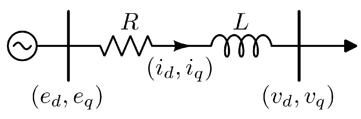
Figure 1 depicts a single-phase equivalent model of a simple power system described in the dq-frame [15,16] and consisting of an infinite bus (which fixes the dq-frame components of its voltage $(e_d,e_q)$ to a given value regardless of power exchange), a line, and a load of two possible kinds: constant power load or constant impedance load. These loads work at the same power level in nominal operating conditions, which implies that the power flow (pf) solution does not change for both load implementations if the voltage at the load bus is at its nominal value.

Figure 1. The single-phase schematic of a simple power system made up of an infinite bus, a line, and a load.

2.1. Small-Signal Models of the Constant Power and Constant Impedance Loads

The equations describing the constant power load are

$${\displaystyle v_d=\frac{i_{d}P-i_{q}Q}{i_d^2+i_q^2},v_q=\frac{i_{q}P+i_{d}Q}{i_d^2+i_q^2},}$$

where P and Q are the loads’ active and reactive power, $(v_d,v_q)$ are the dq-frame components of the bus voltage at which the load is connected, and $(i_d,i_q)$ are the corresponding dq-frame components of the load current.

The constant power load differential impedance at the $({\widehat{i}}_d,{\widehat{i}}_q)$ pf solution is

$$\left[\begin{array}{cc}{\displaystyle \frac{\partial v_d}{\partial i_d}}& {\displaystyle \frac{\partial v_d}{\partial i_q}}\\ {\displaystyle \frac{\partial v_q}{\partial i_d}}& {\displaystyle \frac{\partial v_q}{\partial i_q}}\end{array}\right]=\left[\begin{array}{cc}{R}_p\hfill & \hfill X_p\\ X_p\hfill & \hfill -R_p\end{array}\right],$$

(1)

where

$$R_p=\frac{P\left({\widehat{i}}_q^2-{\widehat{i}}_d^2\right)+2Q{\widehat{i}}_d{\widehat{i}}_q}{{\left({\widehat{i}}_d^2+{\widehat{i}}_q^2\right)}^2}$$

(2)

$$X_p=\frac{Q\left({\widehat{i}}_q^2-{\widehat{i}}_d^2\right)-2P{\widehat{i}}_d{\widehat{i}}_q}{{\left({\widehat{i}}_d^2+{\widehat{i}}_q^2\right)}^2},$$

(3)

with the $^$ symbol denoting values at the pf solution. By representing the $x+\mathrm{J}y$ generic complex number as the ${[x,y]}^{\mathrm{T}}$ two-element real vector, we can derive the ${\tilde{v}}_d^p+\mathrm{J}{\tilde{v}}_q^p$ small-signal voltage obtained by applying a small-signal current perturbation ${\tilde{i}}_d^p+\mathrm{J}{\tilde{i}}_q^p$ as

$$\begin{array}{c}\left[\begin{array}{c}{\tilde{v}}_d^p\\ {\tilde{v}}_q^p\end{array}\right]=\left[\begin{array}{cc}\hfill R_p& \hfill X_p\\ \hfill X_p& \hfill -R_p\end{array}\right]\left[\begin{array}{c}{\tilde{i}}_d^p\\ {\tilde{i}}_q^p\end{array}\right],\hfill \end{array}$$

(4)

where the ${}^p$ superscript refers to the voltages and currents of the constant power load, whereas the $\tilde{}$ symbol denotes small-signal variables.

Consider now the constant impedance load $R_z+\mathrm{J}{X}_z$ with $R_z>0$. Its small-signal voltage is

$$\begin{array}{c}\left[\begin{array}{c}{\tilde{v}}_d^z\\ {\tilde{v}}_q^z\end{array}\right]=\left[\begin{array}{cc}\hfill R_z& \hfill -X_z\\ \hfill X_z& \hfill R_z\end{array}\right]\left[\begin{array}{c}{\tilde{i}}_d^z\\ {\tilde{i}}_q^z\end{array}\right]\hfill \end{array}$$

(5)

where the ${}^z$ superscript refers to the voltages and currents of the constant impedance load. The signs of the matrix in (4) can be equated to those in (5) by imposing

$$\begin{array}{c}\left[\begin{array}{c}{\tilde{v}}_d^p\\ {\tilde{v}}_q^p\end{array}\right]=\left[\begin{array}{cc}\hfill R_p& \hfill -X_p\\ \hfill X_p& \hfill R_p\end{array}\right]\left[\begin{array}{c}\hfill {\tilde{i}}_d^p\\ \hfill -{\tilde{i}}_q^p\end{array}\right].\hfill \end{array}$$

(6)

It is easy to see that this sign rearrangement means that the small-signal voltage of the constant power load can be expressed as ${\tilde{v}}_d^p+\mathrm{J}{\tilde{v}}_q^p=\left(R_p+\mathrm{J}{X}_p\right){\left({\tilde{i}}_d^p+\mathrm{J}{\tilde{i}}_q^p\right)}^{*}$, where the ${}^{*}$ symbol represents the complex conjugation operator. By comparing (5) with (6), one can immediately realize that the small-signal model of the constant power and constant impedance loads are deeply different even when their pf solutions are the same. As will be shown extensively in the following, this implies that the choice of load model may lead to different results in small-signal analyses and transient simulations.

2.2. Power System Small-Signal Stability with Constant Power and Constant Impedance

Let us now study the small-signal stability of the simple power system mentioned at the beginning of this Section. To do so, assume that the line in Figure 1 is described by a dynamic model. In a dynamic load model, the relationship between line voltage and current is described by a differential equation. On the contrary, in a static line model, said relationship is purely algebraic.

When the constant power load is used, the system small-signal behaviour can be modelled by the following differential equation:

$$\begin{array}{c}{\displaystyle \left[\begin{array}{cc}L& 0\\ 0& L\end{array}\right]\frac{d}{dt}\left[\begin{array}{c}{\tilde{i}}_d^p\\ {\tilde{i}}_q^p\end{array}\right]=-\left[\begin{array}{cc}{R}_p& \hfill -X_p\\ X_p& \hfill R_p\end{array}\right]\left[\begin{array}{c}\hfill {\tilde{i}}_d^p\\ \hfill -{\tilde{i}}_q^p\end{array}\right]-\left[\begin{array}{cc}R& -\omega L\\ \omega L& R\end{array}\right]\left[\begin{array}{c}{\tilde{i}}_d^p\\ {\tilde{i}}_q^p\end{array}\right]+\left[\begin{array}{c}{\tilde{e}}_d\\ {\tilde{e}}_q\end{array}\right],}\hfill \end{array}$$

(7)

where $R>0$ and $L>0$ are respectively the resistance and the inductance of the line, $\omega$ is the synchronous angular frequency, and $({\tilde{e}}_d$, ${\tilde{e}}_q)$ are the small-signal components of the infinite bus voltage. The corresponding pair of eigenvalues is

$${\lambda }_{\pm }^p=-\frac{R}{L}\pm \sqrt{\frac{R_p^2+X_p^2}{L^2}-{\omega }^2}.$$

(8)

Through Equations (2) and (3) we obtain the following expression

$$R_p^2+X_p^2=\frac{P^2+Q^2}{{\left({\widehat{i}}_d^2+{\widehat{i}}_q^2\right)}^2}=\frac{\left({\widehat{v}}_d^2+{\widehat{v}}_q^2\right)\left({\widehat{i}}_d^2+{\widehat{i}}_q^2\right)}{{\left({\widehat{i}}_d^2+{\widehat{i}}_q^2\right)}^2}=\frac{{\widehat{v}}_d^2+{\widehat{v}}_q^2}{{\widehat{i}}_d^2+{\widehat{i}}_q^2},$$

which can be used to recast Equation (8) and derive that, if ${\displaystyle \frac{{\widehat{v}}_d^2+{\widehat{v}}_q^2}{{\widehat{i}}_d^2+{\widehat{i}}_q^2}>R^2+L^2{\omega }^2}$, we have instability because one eigenvalue has a positive real part. Otherwise, we have complex conjugate eigenvalues with negative real parts. In both cases, the eigenvalues do not depend on the sign of P and Q.

On the contrary, if we adopt a constant impedance load, the small-signal model becomes

$$\begin{array}{c}{\displaystyle \left[\begin{array}{cc}L& 0\\ 0& L\end{array}\right]\frac{d}{dt}\left[\begin{array}{c}{\tilde{i}}_d^z\\ {\tilde{i}}_q^z\end{array}\right]=-\left[\begin{array}{cc}{R}_z& \hfill -X_z\\ X_z& \hfill R_z\end{array}\right]\left[\begin{array}{c}{\tilde{i}}_d^z\\ {\tilde{i}}_q^z\end{array}\right]-\left[\begin{array}{cc}R& -\omega L\\ \omega L& R\end{array}\right]\left[\begin{array}{c}{\tilde{i}}_d^z\\ {\tilde{i}}_q^z\end{array}\right]+\left[\begin{array}{c}{\tilde{e}}_d\\ {\tilde{e}}_q\end{array}\right].}\hfill \end{array}$$

In this case, the ${\lambda }_{\pm }^z$ eigenvalues are

$${\displaystyle {\lambda }_{\pm }^z=-\frac{R_z+R}{L}\pm \mathrm{J}\left(\omega +\frac{X_z}{L}\right).}$$

(9)

Therefore, the system is stable because both eigenvalues always have negative real parts.

The above results reinforce the point raised in the previous subsection: the adoption of constant power and constant impedance load models leads to different behaviour in small-signal analyses.

2.3. On-Load Tap Changer

This subsection briefly outlines the operating principle of on-load tap changers (oltcs) and reviews their most relevant representations developed in the literature. This element is adopted in some of the scenarios simulated in Section 3.

The target of an oltc is to keep the bus voltage in the predefined dead-band by adjusting the transformer ratio in a given range over a discrete number of tap positions, thereby ensuring that loads connected to them operate at voltage levels close to their rated one. For example, in the oltc model reported in [17], the dead-band can cover the $[0.99,1.01]$ p.u. voltage interval, while the transformer ratio can vary in the $[0.88,1.20]$ interval over 33 discrete positions (i.e., the ratio changes by 0.01 from one position to the next one). The decision process governing the tap control is the following. When the load voltage leaves a dead-band at time $t_0$, the first tap change takes place at time $t_0+{\tau }_1$ and the subsequent ones at times $t_0+{\tau }_1+k{\tau }_2$ with $(k=1,2,\dots )$. The delays ${\tau }_1$ and ${\tau }_2$ have values generally above $20\mathrm{s}$ and can differ from one oltc to another. The delay is reset to ${\tau }_1$ after the controlled voltage (i) has re-entered the dead-band or (ii) has jumped from one dead-band side to the other. The latter criterion prevents the tap from moving if the bus voltage oscillates too much or too frequently compared to the ${\tau }_1$ and ${\tau }_2$ delays.

The interested reader is referred to [18] and references therein for several oltcs representations developed in the literature. The most accurate oltc model, used in this paper, is implemented by a state machine, corresponding to a hybrid dynamical system with a decision block that generates events [19]. The main drawback of adopting this representation is that the pf and transient stability analyses must deal with a digital design that implements the state machine of the oltc, which may lead to a complex simulation approach. In light of this, the majority of the remaining models in [18] were developed to attain a simplified, but still effective, version of oltcs to achieve easy numerical simulations without resorting to a state machine implementation. For instance, the simplest oltc representation (referred to in [18] as a continuous model) adopts a simple first-order differential equation to describe the tap variation process of the oltcs to bring the voltage inside the dead band. So doing, the discrete tap switching process is transformed into a continuous one, thereby disregarding the previously mentioned delays.

It is important to point out that the connection of oltc to loads is a common practice in electric power systems, whose effects are better detailed in the next subsection.

2.4. Conventional Load Modelling in Power System Simulations

The majority of the available power system test benches described in the literature and available on the web use (i) constant power loads and (ii) static models of passive components.

The first feature (i) contrasts with the fact that until the last decade the number of full-fledged constant power loads connected to distribution feeders was practically irrelevant. Thus, based just on the above, this approach seems rather conservative and one would be more inclined to adopt constant impedance load models instead. However, it is worth pointing out that the distribution feeders of electric power systems are often equipped with oltcs (see the previous subsection) that restore voltage levels by bringing them inside a fixed voltage dead-band. Therefore, if only their steady-state behaviour is required (i.e., the pf solution), it seems reasonable to replace constant impedance loads behind oltcs with constant power ones. Indeed, the long-term voltage restoration process of the oltcs implies that at steady-state such loads operate at their nominal voltage and, thus, always withdraw their rated power. Constant power loads correspond somewhat to a synthesis of constant impedance loads behind oltcs. However, it is worth pointing out that the number of loads whose active and reactive power is actually controlled became significant only with the introduction of ibrs (i.e., converter-connected loads (ccls)). Indeed, the converters interfacing these resources to the grid can implement several controls, including power regulation. When ibrs employ this latter control, they constitute full-fledged constant power loads.

Although this modelling approach leads to correct pf results, it may lead to inaccurate transient simulations and small-signal analyses. Indeed, as better shown in the following, constant power loads and constant impedance loads behind oltcs exhibit different dynamic behaviours. The adoption of the former model generally allows considering a worst-case scenario that real conventional power systems tend to. We believe this modelling choice was rooted in the 1970’s when power system simulation tools were first developed [20]. A common practice to overcome the limited capabilities of computers in those years consisted in modelling constant impedance loads behind oltcs as constant power loads to speed up simulations by incurring a minor loss in accuracy. This choice proved extremely effective until recent years when the penetration of ibrs in the power system rose drastically.

Concerning the second feature (ii), the dynamic models of passive components (e.g., transformers, lines, and shunts) were neglected during the development of conventional power system tools since the very fast, purely electrical dynamics of the grid were typically not of concern. This removed the stability problems due to the electrical dynamics of passive elements. Indeed, the electro-mechanical dynamic was the important aspect that had to be accurately simulated. As shown in the following, ibrs implement full-fledged constant power loads and act in a wide frequency bandwidth. This last trait imposes the adoption of dynamic models of passive components to analyse the stability of the system. Indeed, using algebraic models may lead to inaccurate results.

3. Simulation Results of the Conventional ieee14 Power System

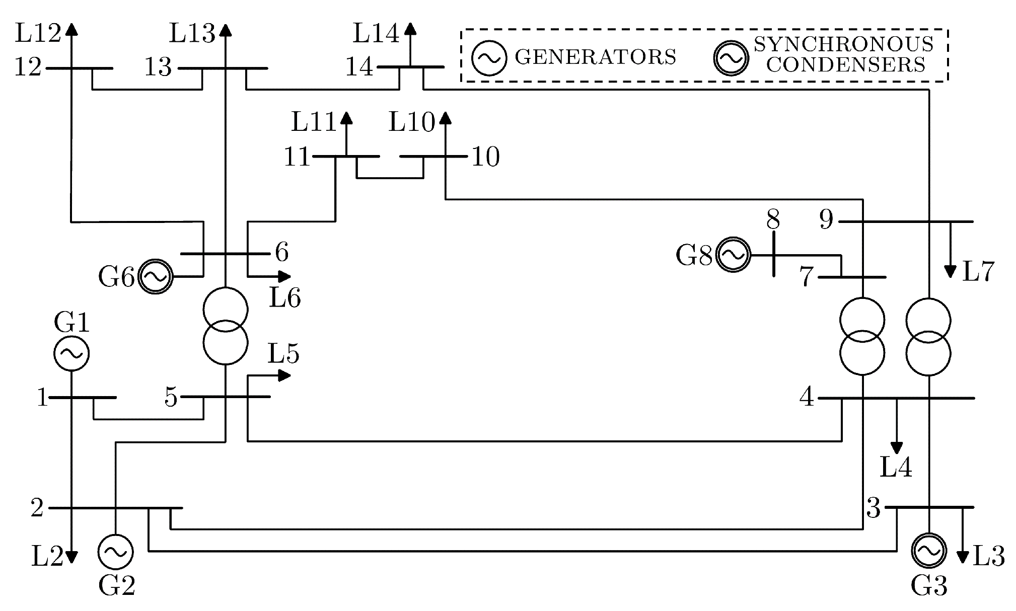
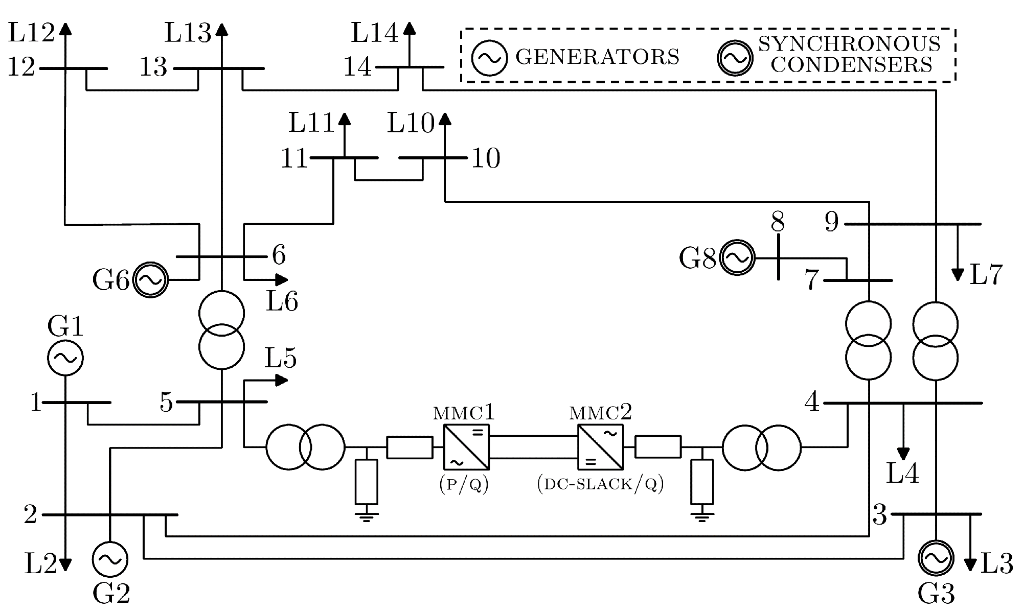
To show the role of constant power and constant impedance load models behind oltcs on stability, we use as a benchmark the well-known ieee14 power system, whose schematic is shown in Figure 2. All the parameters of the conventional version of ieee14 power system can be found in [9].

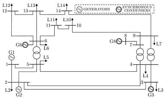
Figure 2. The schematic of the ieee14 power system.

In the following, we modify this benchmark several times to simulate different case studies. In this section, we consider four scenarios. The first one, hereafter referred to as ieee14-p, adopts the conventional version of the ieee14 system with constant power loads. In the second scenario, defined as ieee14-z, we substitute the constant power loads with constant impedance ones behind oltcs, whose nominal transformer ratio equals 1 (i.e., all bus voltages computed at pf are inside the respective dead-bands). The parameters of the constant impedance loads are tuned to absorb the same active and reactive power at the pf solution as the ieee14-p scenario.

It is worth pointing out that the classic version of the ieee14 test system adopts static models of passive elements. Compared to their ieee14-p and ieee14-z counterparts, the third and fourth scenarios, hereafter respectively referred to as ieee14-pd and ieee14-zd, employ dynamic models of inductances and capacitances of power lines, transformers, and shunts. These last two scenarios aim at showcasing the impact of alternative passive element modelling on power system stability.

3.1. The ieee14-p and ieee14-z Scenarios

We performed a transient stability analysis of both ieee14-p and ieee14-z scenarios. In both cases, we tripped the line between bus2 and bus5 after $200\mathrm{s}$ from the beginning of the simulations.

The results of these simulations are shown in Figure 3. By observing the waveforms related to the ieee14-p scenario in the upper panel of the figure, one can notice that when the line is tripped, the rotor angular speed of the G2 synchronous generator suddenly decreases and stabilises after some time just below $0.999\left[\mathrm{pu}\right]$. This behaviour stems from the fact that line tripping induces a load voltage drop and that all the loads in this scenario are of constant power type. Indeed, to guarantee constant power absorption despite the voltage drop, the currents flowing through the loads must increase. This leads to higher currents and power losses across the lines and transformers (and, thus, overall power demand) and, in turn, a decrease in system synchronous frequency. In the specific case of the ieee14 benchmark, which does not implement turbine governors, the system frequency stabilises due to the contributions by damping in the swing equations of the synchronous generators and condensers.

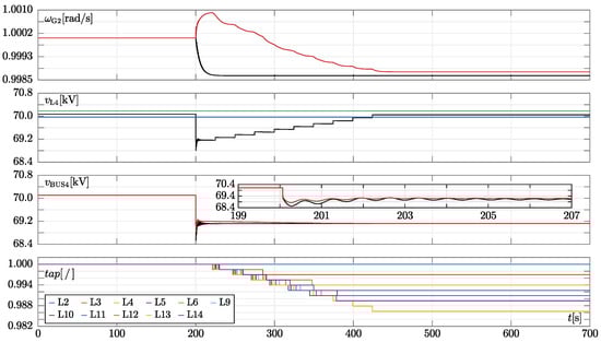
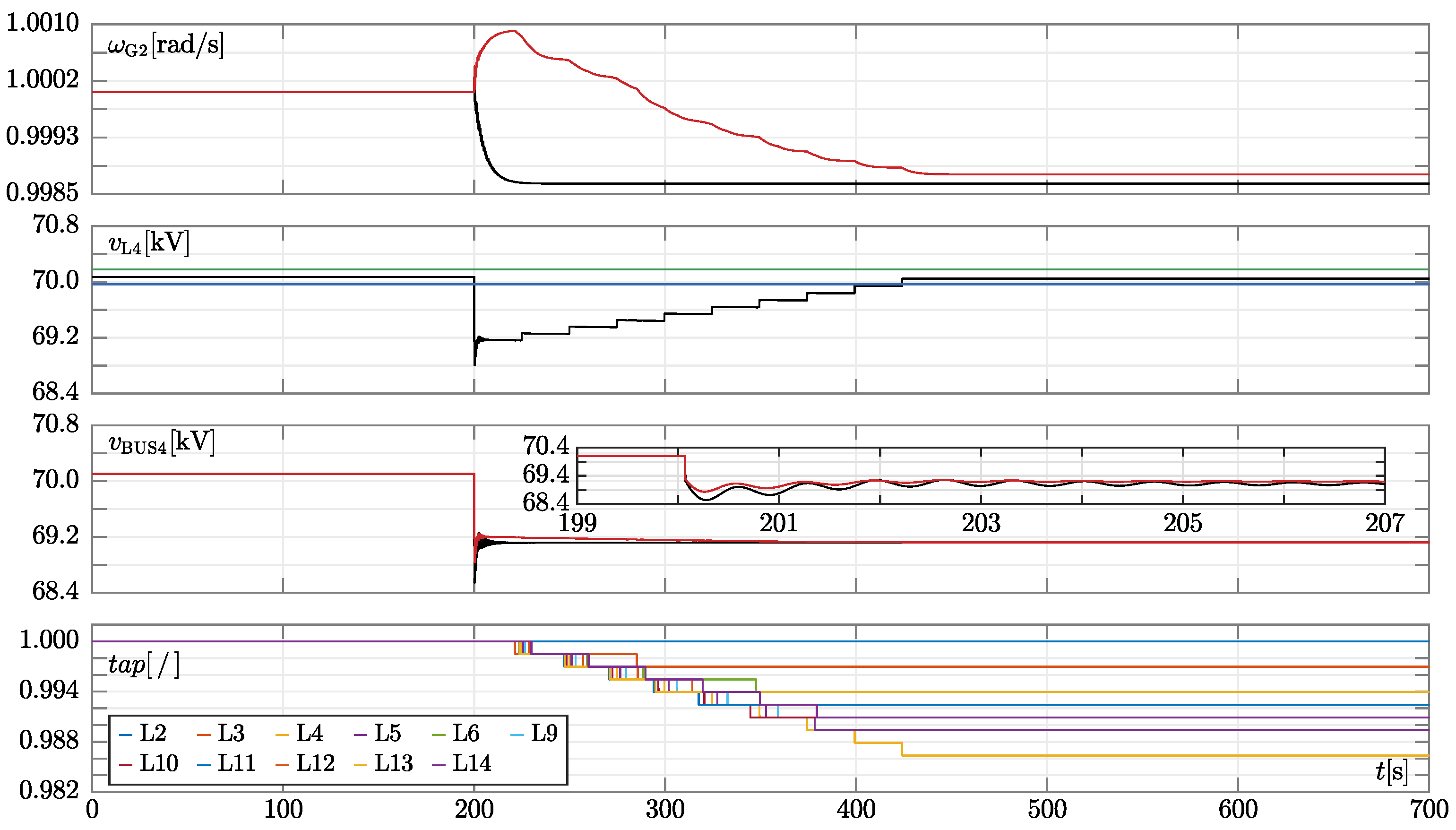
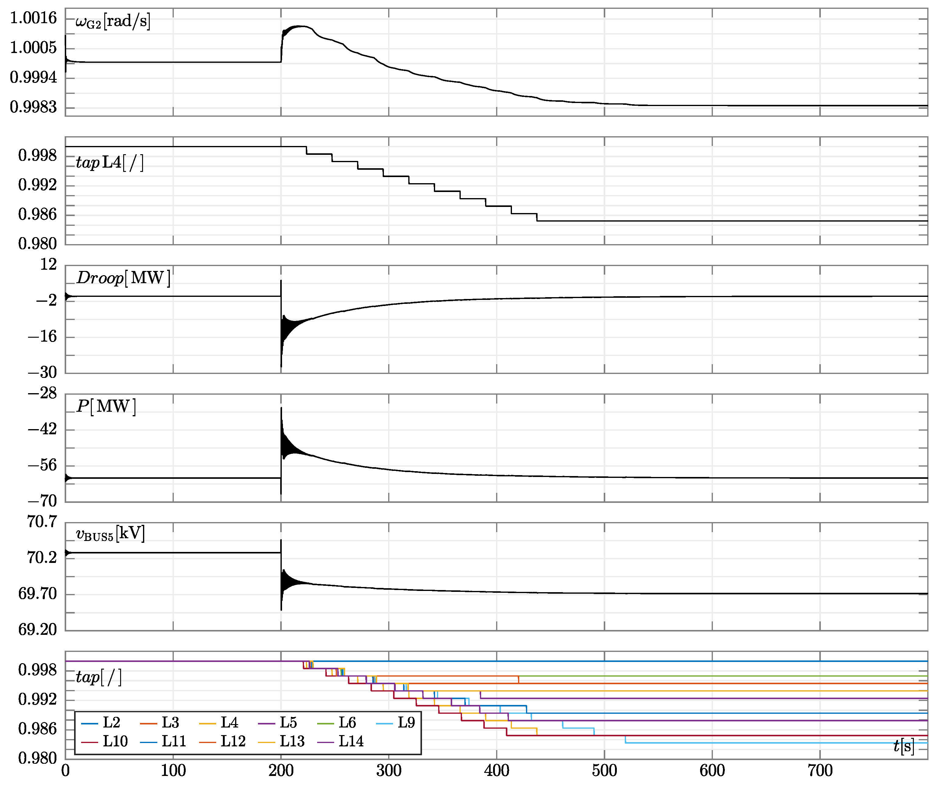
Figure 3. Simulation results of ieee14-p and ieee14-z scenarios. Panels are described below from top to bottom. First panel: rotor angular speeds in [pu] of the G2 synchronous generator in the ieee14-p and ieee14-z scenarios (black and red trace, respectively). Second panel: the black trace corresponds to the voltage magnitude of the constant impedance load l4 when connected to bus4 through an oltc in the ieee14-z scenario, whereas the green and blue traces respectively depict the upper and lower edge of the voltage dead-band inside which the corresponding oltc restores the load voltage. Third panel: voltage magnitude at bus4 in the ieee14-p (black trace) and ieee14-z case studies (red trace). Fourth panel: the tap ratios of the oltcs connected to each load in the ieee14-z scenario. X-axis: time [$\mathrm{s}$].

It is important to note that this phenomenon leads to an iterative process in which the increase in line currents determines a decrease in load voltage, which, in turn, yields a further increase in line currents. Eventually, this process converges into a new stable working mode of the ieee14-p scenario, as shown by the magnitude of the bus4 voltage in Figure 3 (third panel from the top, black trace).

Consider now the ieee14-z scenario: contrary to the ieee14-p case, the rotor speed of the G2 synchronous generator increases instead of decreasing right after the line tripping. Analogously to the previous scenario, this behaviour is coherent with the load model adopted and line tripping resulting in a load voltage drop. For instance, if we observe the magnitude of the voltage at bus4 (third panel from the top), also in this scenario it decreases just after line tripping (although slightly less than in the ieee14-p case). Since the power absorbed by constant impedance loads varies quadratically with voltage, the decrease in load voltage magnitudes leads to lower load powers. This implies that the currents flowing through the loads, lines, and transformers decrease. The same holds for the overall power demand, thereby leading to an increase in frequency, which stabilises once again due to the damping of the synchronous generators and condensers.

The traces in the second panel from the top in Figure 3 show that after some time delay the oltc at bus4 starts restoring the load voltage till bringing it inside the voltage dead-band (i.e., almost full voltage restoration to its value before the line outage is attained). As shown in the last panel of the figure, the other oltcs do the same with different time schedules. The load voltage restoration process causes a progressive step increase in the power of the constant impedance loads and, thus, a corresponding decrease in grid frequency. At the end of this (long-term) process lasting more than $400\mathrm{s}$ (see traces of the other oltc in the last panel of Figure 3), the steady-state behaviour of the power system is very close to that of the ieee14-p case, but not identical, since load voltages are set to different values inside the oltc dead-bands.

Similar results were already reported in [9], although with different and simpler oltc models [18,21]. The previously described scenarios highlight that if the analysis focuses exclusively on power system steady-state behaviour (i.e., pf results), constant power loads can be adopted instead of constant impedance ones behind oltcs, thus boosting simulation efficiency at the expense of a minor accuracy loss. However, if the dynamic behaviour is of interest (i.e., transient simulations or small-signal analyses are executed), these two models are not equivalent and may lead to quite different results. For instance, this difference is evident when applying a $20\%$ overload to the ieee14-p and ieee14-z scenarios and tripping the line between bus2 and bus5. In the first case, as reported in [9,22], the system pf solution is characterised by a pair of complex conjugated eigenvalues with positive real part equal to $0.006268\pm \mathrm{J}1.4357$ after line tripping, and thus it becomes unstable. On the contrary, in the second case, the system remains stable despite the overload (i.e., all eigenvalues have a negative real part before and after line tripping). In particular, the grid in this case can withstand a $58\%$ overload before becoming unstable.

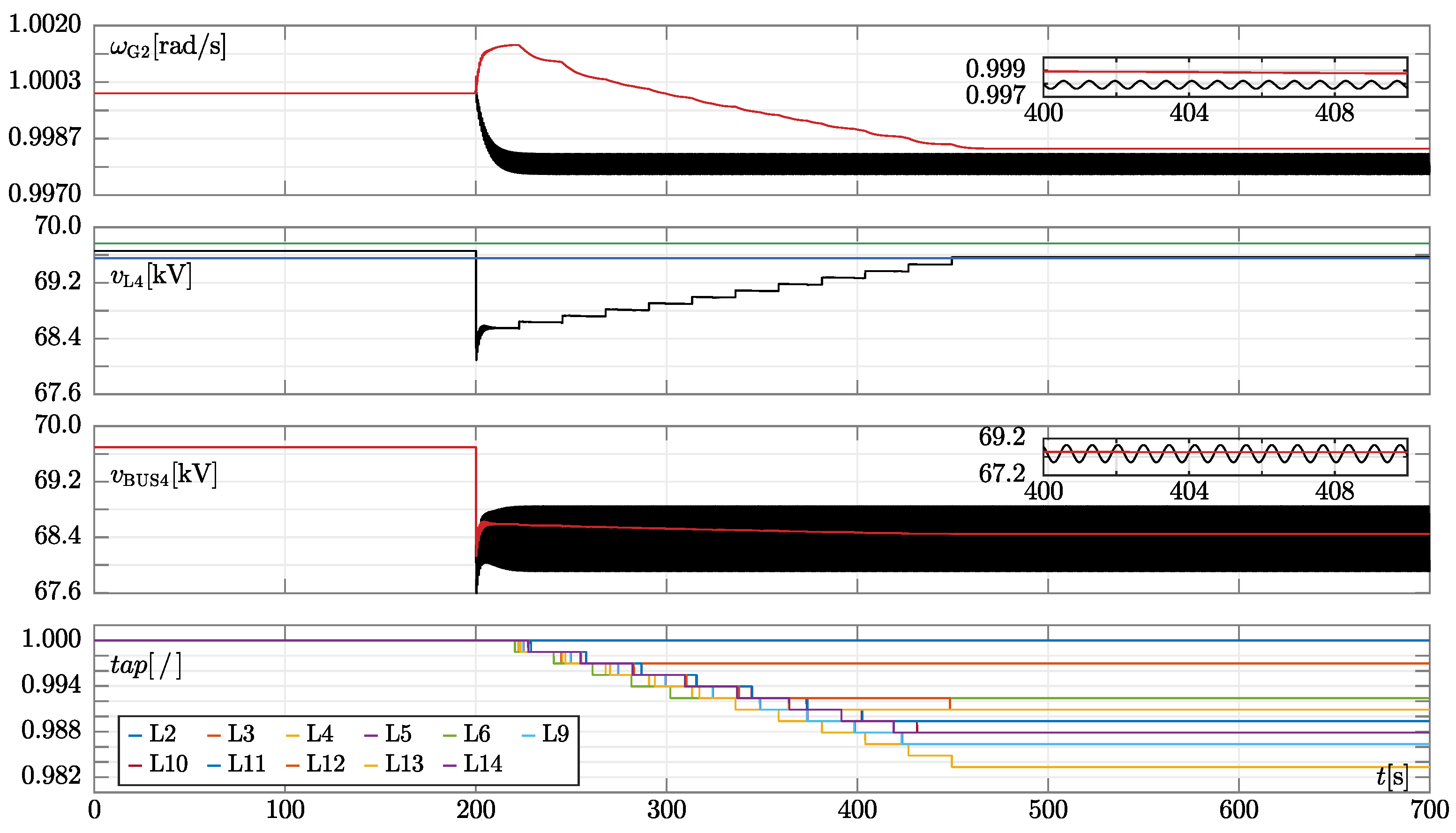
To confirm these completely different results, we performed a transient stability analysis of the ieee14-p and ieee14-z case studies by applying a $20\%$ overload. Based on the above, we predict that the former scenario shall become unstable after applying a disturbance (i.e., line tripping), while the latter remains stable. A similar approach is used in the following section to demonstrate the actual stability or instability of the ieee14 benchmark in other simulated scenarios after performing an eigenvalue analysis. Results are reported in Figure 4.

Figure 4. Simulation results of ieee14-p and ieee14-z scenarios when a $20\%$ overload is applied. The traces in each panel have the same meaning as those in Figure 3. Insets in the first and third panels are meant to show the oscillations that arise in the ieee14-p scenario.

As expected, after line tripping, the rotor speed of G2 in the ieee14−p scenario (black trace in the upper panel of Figure 4) starts oscillating, indicating that a periodic steady-state behaviour is observed since a stable stationary solution is not reached (i.e., the grid becomes “unstable”). As shown by the black trace in the third panel from the top, the voltage magnitude of bus4 also oscillates. The same holds for the voltage at other buses, too. On the contrary, after line tripping, the grid in the ieee14-z scenario remains stable, without showing any oscillations. Note that oltcs “fully” restore load powers and thus the absence of oscillations can not be ascribed to the fact that the power of constant impedance loads are lower after line tripping.

In summary, the results in the two case studies confirm that the use of constant impedance loads behind oltcs instead of constant power ones leads to completely different stability results for what concerns both small-signal analyses and transient simulations. Based on this observation, one might wonder which load model actually correctly and accurately represents the real behaviour of the ieee14 system and possibly other grids. To answer this question, we believe the following points are worth considering.

(i) The use of constant power load models leads to pessimistic estimations of the stability boundary conditions. From an engineering point of view, this could be a good feature since it gives safety margins. From this perspective, despite leading to inaccurate results, constant power load models can still be considered adequate and useful.

(ii) The use of constant power loads eliminates the need to implement the complex automata modelling the behaviour of oltcs connected to constant impedance loads, which simplifies power flow and transient stability analyses and reduces the computational burden.

(iii) The tap switching process of the oltcs occurs after relatively long time periods (i.e., tens of seconds). Thus, since the power restoration of the constant impedance loads connected to the oltcs is a decidedly slow process, the electrical dynamics of passive elements can be neglected. Indeed, the only dynamics that should be considered are the electro-mechanical ones of the generators, which are retained when adopting constant power loads. Also, in this case, employing algebraic (i.e., static) models of passive elements facilitate and accelerate simulations while ensuring adequately accurate results.

The above considerations lead to the conclusion that the use of (i) constant power loads instead of constant impedance ones behind oltc in distribution feeders and (ii) algebraic models of passive elements instead of dynamic ones have become customary in modelling and simulating power systems till today. However, this established practice may no longer be valid due to the increasing presence of ibrs. Indeed, due to the controls that they can implement, ibrs may represent fast constant power loads and generation; their ac impedances, which might be complex functions of frequency spanning in the range of several $\mathrm{kHz}$, can deeply interact with the dynamics of passive elements. If algebraic models are used, these interactions may remain hidden; thus, simulations may not accurately reflect the true behaviour of the system. This aspect, which is dealt with in the following, suggests that the conventional model of loads and passive elements may require revision when used in ibr-dominated grids.

3.2. The ieee14-pd and ieee14-zd Dynamic Test Systems

The case studies analyzed so far relied on static models of lines. In the following, we adopt dynamic line models by considering the ieee14-pd and ieee14-zd scenarios and simulating the same outage described in the previous subsection (i.e., line tripping between bus2 and bus5 at $200\mathrm{s}$).

The ieee14-pd case gives extremely straightforward results: the adoption of dynamic models and constant power loads yields an unstable pf solution since several eigenvalues jump in the right-half portion of the complex plane. Note that this result anticipates that the introduction in the system of ibrs (e.g., mmcs), whose active and reactive power absorption is regulated to track a reference value (thereby mimicking constant power loads), will lead to similar instabilities. Since the attainment of an unstable pf solution prevents any further analysis of this case study, in the sequel we consider only the ieee14-zd scenario.

In this case, a completely different result is obtained because the pf solution is stable. The different behaviours observed in the ieee14-pd and ieee14-zd scenarios are coherent with what we obtained by computing the eigenvalues of Equations (7) and (9). Indeed, as explained in Section 2.1, power systems with constant power loads are less robust than those with constant impedance ones from a stability point of view. To facilitate comparisons, the simulation results of the ieee14-z scenario are replicated in Figure 5 together with those of the ieee14-zd one.

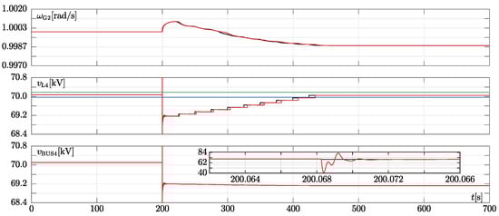
Figure 5. Simulation results of ieee14-z and ieee14-zd scenarios. The traces in each panel have an analogous meaning to those in Figure 3. In this case, the black and red traces in each panel respectively refer to the results of the ieee14-z and ieee14-zd scenarios. In the second and last panel, the voltage magnitude of bus4 is upper and lower clipped to better show voltage steps at a tap position change.

The traces in the two cases almost overlap despite them adopting two different line models. It is worth pointing out that in Figure 5 the magnitude of the bus4 voltage is clipped (upper and lower) to allow a better comparison of the waveform in the two cases. The inset in Figure 5 depicts the unclipped voltage magnitude just before and right after the line tripping.

4. Simulation Results of the Modified ieee14 Power System with an mmc-Based hvdc Link

In this section, we show some simulation results of a modified version of the ieee14 system. To take into account the effect of the growing presence of ibrs on power system stability, the line between bus4 and bus5 was replaced with an hvdc link comprising two mmcs, as shown in Figure 6.

Figure 6. The schematic of the modified ieee14 power system. Compared to its counterpart in Figure 2, the line between bus 4 and 5 has been substituted with an hvdc link made up of two mmcs.

This modification was proposed and described in [23,24,25]. In a nutshell, the mmc1 and mmc2 converters are respectively of p/q and dc-slack/q types. In other words, mmc1 is controlled to exchange a specific amount of active and reactive power. On the contrary, mmc2 regulates the dc-side voltage and reactive power exchange. In particular, the active and reactive power transmitted by the hvdc link is regulated to equal that of the replaced line. To do so, the active power reference value of mmc1 (i.e., sending end) is $P_o=60.7\mathrm{M}\mathrm{W}$, while the reactive power reference value of both mmcs is $Q_o=\mp 13\mathrm{M}\mathrm{VAR}$. In addition, the dc-side voltage reference value of mmc2 (i.e., receiving end) is $V_{dc}=400\mathrm{k}\mathrm{V}$. The interested reader is referred to Figure 1 of [26] and references therein for a possible mmc control scheme implementation.

When employed in hvdc systems, the sub-modules (sms) in each arm of an mmc can be in the order of hundreds. In this case, adopting the most accurate mmc model (known as full-physics model) requires considering a large number of semiconductor devices, thereby leading to prohibitively high computational times [27]. To address this issue, several mmc models in the literature have been developed that implement different trade-offs between simulation speed and accuracy. Each of these models is better suited for analysing the efficiency of specific operating conditions and mmc controls (e.g., circulating current suppression strategies, protections, plls, and sm capacitor voltage balancing algorithms [28,29]). The interested reader can refer to [30,31,32] and references therein for a review of some of these models, including a description of their advantages and shortcomings when adopted in power system simulation.

In general, the analysis of converters can be divided into three stages [27]: component, system, and network level studies. Component level studies focus on the early design stage of the converter and the performances of its semiconductors (e.g., conduction and switching losses), with the time of investigation ranging from nano to milliseconds. On the contrary, system-level studies aim at evaluating the interactions between the converter and the power system connected to it, whose extension is usually limited to a few generators and loads. These analyses, which involve dynamics that last from milliseconds to several seconds, allow the validation of converter controls, filters, and protections. Finally, network-level studies analyse how the converter behaves in a large ac network and affects the electromechanical transients and the steady-state operation of the whole system. Thus, the time interval of interest ranges from a few seconds to several minutes. Such studies address, for instance, power flow and stability analyses.

The full-detailed and bi-value resistor mmc models allow reducing cpu times by resorting to simplified representations of the semiconductor devices in each sm, thus preserving the overall converter topology [30]. These models can be used as a benchmark to validate simpler ones, test mmc controls, protections, and behaviour during start-up, normal and abnormal operating conditions. However, due to the simplifications introduced, these representations cannot be used for component-level studies, which can only be performed straightforwardly with the full physics model.

The Thévenin equivalent [33] and switching function [34] models, which still rely on simplified sm representations, are good candidates for system-level studies because they further boost simulation speed by suitably grouping the sms together, thus obtaining a more compact representation of the sm strings in each arm. Alternatively, in [32] a technique called isomorphism is proposed to boost mmc simulation efficiency that is compatible with any sm model used, thereby paving the way for detailed analyses if accurate sm representations are used. In a nutshell, this technique dynamically clusters while simulating the sms in groups characterised by the same behaviour.

The average model decreases simulation time even more by neglecting the voltage and current ripples due to sms commutations [35] and significantly simplifying the mmc topology by exploiting voltage and current controlled sources. This model is suitable for network-level studies which investigate the dynamic behaviour and stability of large grids comprising multiple mmcs.

All of the models described so far are represented in the abc (i.e., three-phase) frame. On the contrary, mmc models formulated in the dq0 frame, either based on an average representation [36] or dynamic phasors [37], grant a significant boost in simulation speed, making them suitable candidates for mmc simulation in large-scale power systems.

In general, the boost in simulation speed offered by the mmc models mentioned above may come at the cost of reduced simulation accuracy and/or the loss of internal mmc variables, which are no longer present due to the simplifications introduced in the sm model and the mmc topology. As previously stated, based on the study that needs to be performed (and, thus, the sought trade-off between simulation speed and accuracy), one mmc model might be more suitable than others.

In this paper, we modelled the mmcs of the hvdc system at two very different levels of accuracy: the former, hereafter referred to as accurate, is shown in Figure 1a–c of [26] and derives from [38]. This three-phase model substitutes the sms in each arm of the mmc with a single equivalent circuit. It retains the main features of the converter and allows analyzing all of its upper-level controls, as well as the circulating current suppression strategy. The usage of an average model instead of one based on dynamic phasors is justified by the relatively limited size of the ieee14 benchmark system. In addition, more complex mmc models, which allow us to analyse the individual behaviour of sms, have not been adopted because their level of detail is excessive for the simulations described in the following sections. The second mmc model used in this work (hereafter referred to as simplified) is the one described in [39,40], which resorts to macro-models that retain only the main features at the points of connection of the converters and allow only the implementation of higher-level controllers, such as active and reactive power regulations and droop controls. This representation corresponds to an average model formulated in the dq-frame. Some of its components are added to properly take into account the converter losses at the ac and dc sides. Despite leading to a lower computational burden, one of the drawbacks of this model is that it does not consider any dynamics. Indeed, the impedances connected to its ac side (e.g., the mmc transformer impedance) are referred to as the synchronous frequency and are fixed (i.e., they do not change with grid frequency). As shown in the following, this static model constitutes a deep simplification that could lead to largely different simulation results from those obtained with a more accurate mmc model. Indeed, the complex topology and control scheme of mmcs result in them having a multi-frequency response generating non-negligible harmonics.

Regardless of the representation employed, the key aspect of the analyses with these mmc models is that the mmc1 converter at bus5 is always a full-fledged p/q type. Even if a simplified version of the converter is used, its main features at the point of connection to the ac grid (i.e., absorbing a constant active power of $P_o=60.7\mathrm{M}\mathrm{W}$ and contributing a reactive power of $Q_o=-13\mathrm{M}\mathrm{VAR}$) are maintained. This represents the main difference with respect to the previously considered cases.

We want to stress that our goal here is not to investigate in detail all the possible controls that can be implemented in mmc1 and mmc2, but rather to show the impact that the two previously described mmc models and their controls might have on the overall power system stability in different scenarios.

4.1. Simplified mmc Model

To begin with, we used the simplified model of the mmcs, which, as previously stated, does not consider any dynamics. We instead considered the electrical dynamics of passive components, adopted constant impedance loads behind oltcs, and swept the active power absorbed by the p/q type mmc1 converter in the $[0,P_o]$ interval.

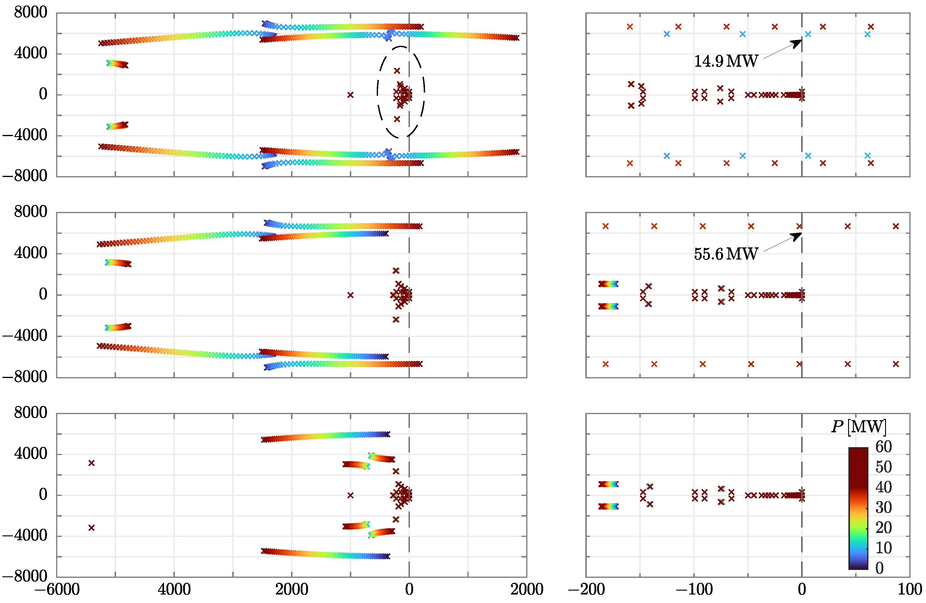
The reactive power of both mmcs was also swept in proportion accordingly. At each sample of the sweep, we performed an eigenvalue analysis. The top panel of Figure 7 reports the paths followed in the complex plane by the most relevant eigenvalues of the system (i.e., those closest to the right-half portion of the complex plane).

Figure 7. Evolution of the main eigenvalues of the ieee14 power system shown in Figure 6 when the active power reference P of the p/q type mmc1 converter at bus5 is swept in the $[0,60.7\mathrm{M}\mathrm{W}]$ interval. For each row, the panels on the right are an inset of those on the left. The vertical dotted line in each panel denotes the null real part of the eigenvalues. Eigenvalues are colour-coded based on P (see the colour bar in the bottom panel, right side) to better identify the power reference values that make the system unstable, which are highlighted by arrows in the panels on the right. Top row: base case. The real part of the eigenvalues inside the dashed ellipse is close to zero, but it is always negative regardless of P (the same holds for the other panels). Middle row: case in which mmc1 includes the droop control and low-pass filter described in Equation (11). Bottom row: compared to the previous case, a shunt capacitor is also added to the ac-side of mmc2. In all cases, dynamic models of lines and transformers are used, together with constant impedance load models behind oltcs.

During the sweep, as soon as the active power goes above $14.9\mathrm{M}\mathrm{W}$, the power system becomes unstable since a complex-conjugate pair of eigenvalues with a natural frequency of about $1\mathrm{k}\mathrm{Hz}$ enters the right-half portion of the complex plane. It is worth pointing out that this power value is lower than the one the hvdc link is supposed to transmit (i.e., $P_o=60.7\mathrm{M}\mathrm{W}$). The onset of unstable behaviour at around $14.9\mathrm{M}\mathrm{W}$ is visible in the top panel of Figure 7: eigenvalues are colour-coded based on the active power reference value. Moreover, when the active power sweep reaches $55.6\mathrm{M}\mathrm{W}$, another complex conjugate pair of eigenvalues enters the right-half plane.

The unstable pairs of complex-conjugate eigenvalues that arise at $14.9\mathrm{M}\mathrm{W}$ and $55.6\mathrm{M}\mathrm{W}$ are due to different reasons, which have been identified through the analysis of the participation factors. In the former case, results indicate that instability is mainly due to bus5 and the line that connects bus2 and bus5 [41,42,43] (i.e., where the p/q type mmc1 is connected). On the contrary, in the latter case, the participation factors show that the second unstable mode is mainly due to bus4 and the line that connects bus3 and bus4 (i.e., where the dc-slack/q type mmc2 is connected). The relevant aspect that we underline is that the mmc1 and mmc2 converters are not unstable per se but they are when used in the ieee14 benchmark due to their interactions with the grid.

For instance, a qualitative explanation of the onset of instability at bus5 due to the p/q type mmc1 is the following. From (1) and (2) it can be inferred that the mmc1 is characterised by a negative resistance, which is a common trait of converter-connected elements whose active and reactive power absorption is regulated. In the specific case of the ieee14 benchmark, when the mmc1 active power reference exceeds $14.9\mathrm{M}\mathrm{W}$, its negative resistance becomes higher than the series resistance of the lines/transformers, thereby leading to undamped rlc oscillations [44].

A possible way to keep the eigenvalues of the mmc1 in the left half-plane is to regulate its actual active power exchange by adding an ac-voltage/active power droop. More specifically, with the addition of the droop the power absorbed by this converter becomes

$$P\left(t\right)=P_o+{\gamma }_P\stackrel{{\displaystyle e\left(t\right)}}{\overbrace{\left(\sqrt{v_d^2\left(t\right)+v_q^2\left(t\right)}-\sqrt{{\widehat{v}}_d^2+{\widehat{v}}_q^2}\right)}},$$

(10)

where the electrical quantities refer to bus5 and ${\gamma }_P>0$. This latter parameter mirrors the constant of the proportional regulator used in the mmc to implement the droop. This control is such that the absorbed power P rises if the modulus of the bus5 voltage increases with respect to its value at the pf solution (i.e., ${\displaystyle \sqrt{{\widehat{v}}_d^2+{\widehat{v}}_q^2}}$) and vice versa otherwise. The introduction of the droop emulates a “constant impedance” load, which absorbs $P_o$ at nominal bus voltage.

Since the droop modifies the mmc1 active power set-point (i.e., its transmitted power), we added a low-pass filter block to slowly restore power to its $P_o$ nominal value. The overall model implementing the regulator is

$$\begin{array}{c}{\displaystyle {\tau }_L\frac{dx\left(t\right)}{dt}+x\left(t\right)-e\left(t\right)=0}\hfill \\ P\left(t\right)=P_o+{\gamma }_P\left(e\left(t\right)-x\left(t\right)\right),\hfill \end{array}$$

(11)

whose transfer function is ${\displaystyle H\left(s\right)=\frac{P\left(s\right)}{e\left(s\right)}={\gamma }_P\frac{{\tau }_{L}s}{1+{\tau }_{L}s}}$. The addition of the low-pass filter emulates the same effects that an oltc has on the restoration of the voltage, and, thus, power of a constant impedance load connected to it. In the light of the above, the combination of the droop and the low-pass filter transforms the p/q type mmc1 into a constant impedance load behind an oltc.

After this modification, we repeated the power sweep analysis that we did before. The loci described by the most relevant eigenvalues are reported in the middle panel of Figure 7. The beneficial effect due to the introduction of the droop and low-pass filter block is evident. Indeed, the unstable complex-conjugate pair of eigenvalues that previously arose at $14.9\mathrm{M}\mathrm{W}$ is now absent.

However, the eigenvalue pair that enters the right-half plane when $P_o$ goes above $55.6\mathrm{M}\mathrm{W}$ is still present. The analysis of the participation factors confirms again that this pair is due to the dc-slack/q type mmc2 converter connected at bus4. To eliminate this pair it is necessary to act on mmc2 by modifying its equivalent impedance “seen” at its point of connection. In this case, we added a shunt capacitor to mmc2 to obtain stability. The eigenvalues loci of the power system after this intervention are shown in the bottom panel of Figure 7. The addition of shunt capacitors is clearly beneficial because all eigenvalues remain in the left-half plane regardless of the active power reference value.

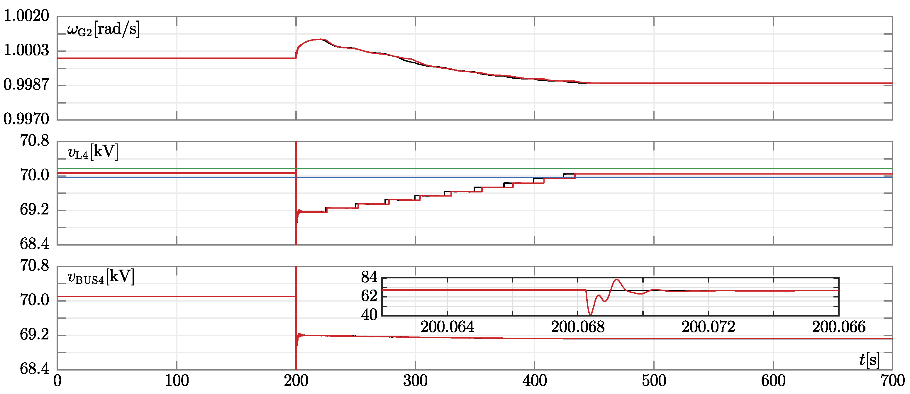
To further check stability, we performed a transient stability analysis analogous to those of Section 3, whose results are reported in Figure 8.

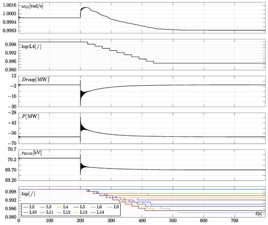
Figure 8. Simulation results of the modified ieee14 test system shown in Figure 6. In this case, constant impedance loads behind oltcs and dynamic line models are used. The mmc1 converter, which is equipped with an ac-voltage/active power droop, is set to exchange $P=60.7\mathrm{M}\mathrm{W}$ and $Q=-13\mathrm{M}\mathrm{VAR}$ (this latter value is also exchanged by mmc2). The mmc2 converter is equipped with a shunt capacitor. Third panel from the top: mmc1 power exchange variation due to the implementation of the droop control. Fourth panel: overall power exchange of the mmc1 converter. The traces in the other panels have the same meaning as those in Figure 3.

As in the previously analysed scenarios, when the line between bus2 and bus5 is tripped at $200\mathrm{s}$, a voltage drop occurs at all buses, including bus4 and bus5. This leads to a decrease in the load power absorbed by the constant impedance loads. In addition, the droop controller of mmc1 lowers its absorbed power in a similar way. From the same figure, one can notice that the long-term load voltage restoring action of the converter is similar to those of oltcs. This was obtained through a proper tuning of the ${\tau }_L$ time constant in Equation (11).

4.2. Accurate mmc Model

In this section, we used the dcs1 test system by CIGRE as a detailed three-phase model of the mmc-based hvdc link. Its schematic, which is fully described in [27], is not reported here for space reasons. The original power rating of the dcs1 system is $800\mathrm{M}\mathrm{W}$, which is abundant for our scope: indeed, it is worth recalling that the hvdc link in Figure 6 is meant to transmit $60.7\mathrm{M}\mathrm{W}$. Therefore we reduced the power rating to $100\mathrm{M}\mathrm{W}$. The three-phase transformers of both mmcs were adapted to step-up voltage from $69\mathrm{k}\mathrm{V}$ to $145\mathrm{k}\mathrm{V}$ and $380\mathrm{k}\mathrm{V}$ respectively to meet the original design requirements. The pll of each mmc tracks the frequency at the point of connection and aligns to the q-axis of the dq-frame.

To have some insight into the behaviour of the system and to understand the mutual interactions between the power system and the mmcs when a more accurate three-phase mmc model is used together with constant impedance loads, we computed the admittances of mmc1 and mmc2 at their points of connections and checked for possible stability issues [45,46,47]. Note that we deal with a hybrid model of the ieee14 system, where the mmcs are simulated with detailed three-phase dynamic models and the ieee14 with a single-phase equivalent model. A conventional eigenvalue analysis can not be performed with this hybrid power system.

At first, we chose the $P=11.2\mathrm{M}\mathrm{W}$, $Q=\mp 2.6\mathrm{M}\mathrm{VAR}$ set-points and connected each step-up transformer to an infinite bus. This is the common configuration used to design an hvdc link and its converter stations that will be connected to ac systems. The adoption of such a configuration ensures that the hvdc link and its mmcs are designed to be stable per se. However, as explained in the following, this does not prevent possible undesired grid and converter interactions from occurring when the hvdc link is connected to a real power system, such as the ieee14 one. The choice of the set-points is based on the top panel of Figure 7: since with these setpoints no eigenvalue has a positive real part, system stability should be ensured.

The numeric tool we used to compute admittances is fully described in [26] and implemented in our own simulator pan [48,49]. In extreme synthesis, a small-signal tone with variable frequency is injected in one of the three phases of the step-up transformer (in our case the “a” phase) of each mmc. This tone superimposes the phase voltage (of large magnitude). We computed the corresponding phase current, extracted the small-signal current contribution due to the injected small signal, and computed the admittance (i.e., the current versus voltage small-signal transfer function).

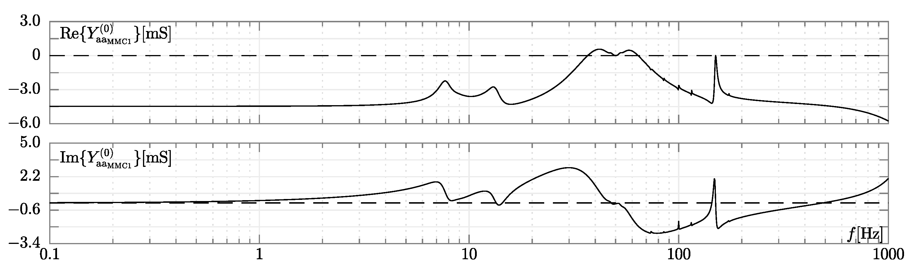
The plots in Figure 9 depict the real and imaginary components of the admittance of the p/q type mmc1.

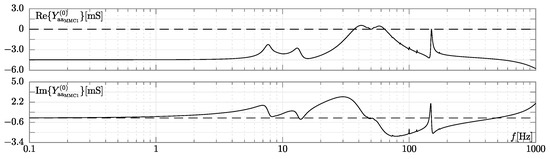
Figure 9. The admittances of the “a” phase of the p/q type mmc1 when the accurate mmc model is used. Upper panel: real part of the admittance [$\mathrm{m}\mathrm{S}$]. Lower panel: imaginary part [$\mathrm{m}\mathrm{S}$]. X-axis: frequency [$\mathrm{Hz}$]. In the panels, the dashed lines denote null real and imaginary parts.

The plots include several frequency intervals, both at low and high frequencies, where the real part of the admittance is negative and its imaginary part is positive (capacitive behaviour). In Figure 10 we report the admittance of mmc2.

Figure 10. The admittances of the “a” phase of the dc-slack/q type mmc2 when the accurate hvdc link model is used. Upper panel: real part of the admittance [$\mathrm{m}\mathrm{S}$]. Lower panel: imaginary part [$\mathrm{m}\mathrm{S}$]. X-axis: frequency [$\mathrm{Hz}$]. In the panels, the dashed lines denote null real and imaginary parts.

The traces are similar to the corresponding ones in Figure 9, but their magnitudes are about ten times lower. Thus, since mmc1 potentially exhibits the largest negative conductance in both low and high-frequency intervals, it constitutes the most critical mmc from a system stability perspective. In particular, as suggested in the previous subsection, (i) mmc1 can form an unstable RLC resonator with the inductances of the lines and transformers (i.e., when dynamic models of passive elements are used). This phenomenon might occur at frequencies higher than those at which ac grids typically operate. In addition, (ii) mmc1 can even interact with the models of synchronous generators/condensers of the ieee14 power system leading to poorly damped or unstable (electro-mechanical) low-frequency modes (less than $10\mathrm{Hz}$).

To provide more details about the first comment (i), consider the high-frequency portion of the admittance of mmc1 in Figure 9. For example, at $1\mathrm{k}\mathrm{Hz}$ its susceptance is about $2.04\mathrm{m}\mathrm{S}$ (corresponding to $0.324\mathsf{\mu }\mathrm{F}$ equivalent capacitance), while its conductance is negative. If the line inductance is larger than $80\mathrm{m}\mathrm{H}$ (a value attainable with an overhead line of sufficient length, such as $100\mathrm{k}\mathrm{m}$), an unstable rlc equivalent circuit can originate [50]. This happens even at relatively low power levels since the detailed model of the mmc shows a much more complex admittance function with respect to its simplified counterpart. This kind of instability can be avoided at high frequency provided that the L inductance of the transformers and the lines is sufficiently low. It is also important to note that this instability does not occur when non-dynamic line and transformer models are adopted. Indeed, in this case, the inductance would be null, thereby preventing the unstable RLC resonator from originating.

Now, to further elaborate on the second comment (ii), consider the lower-frequency portion of the admittance in Figure 9. The admittance has a negative real part and positive imaginary part at frequencies less than $10\mathrm{Hz}$. This means that undesired interactions among mmc1 and the electro-mechanical dynamics of synchronous generators and condensers can arise. These interactions are known as sub-synchronous oscillations (sso) and are similar to sub-synchronous resonances [51,52,53]. Contrary to the previously mentioned instability issues at high frequencies, sso cannot be effectively prevented by acting on L. Indeed, to do so, L should assume values impractical to obtain. In addition, as better shown in the following, ssos depend on the mmc active power exchange.

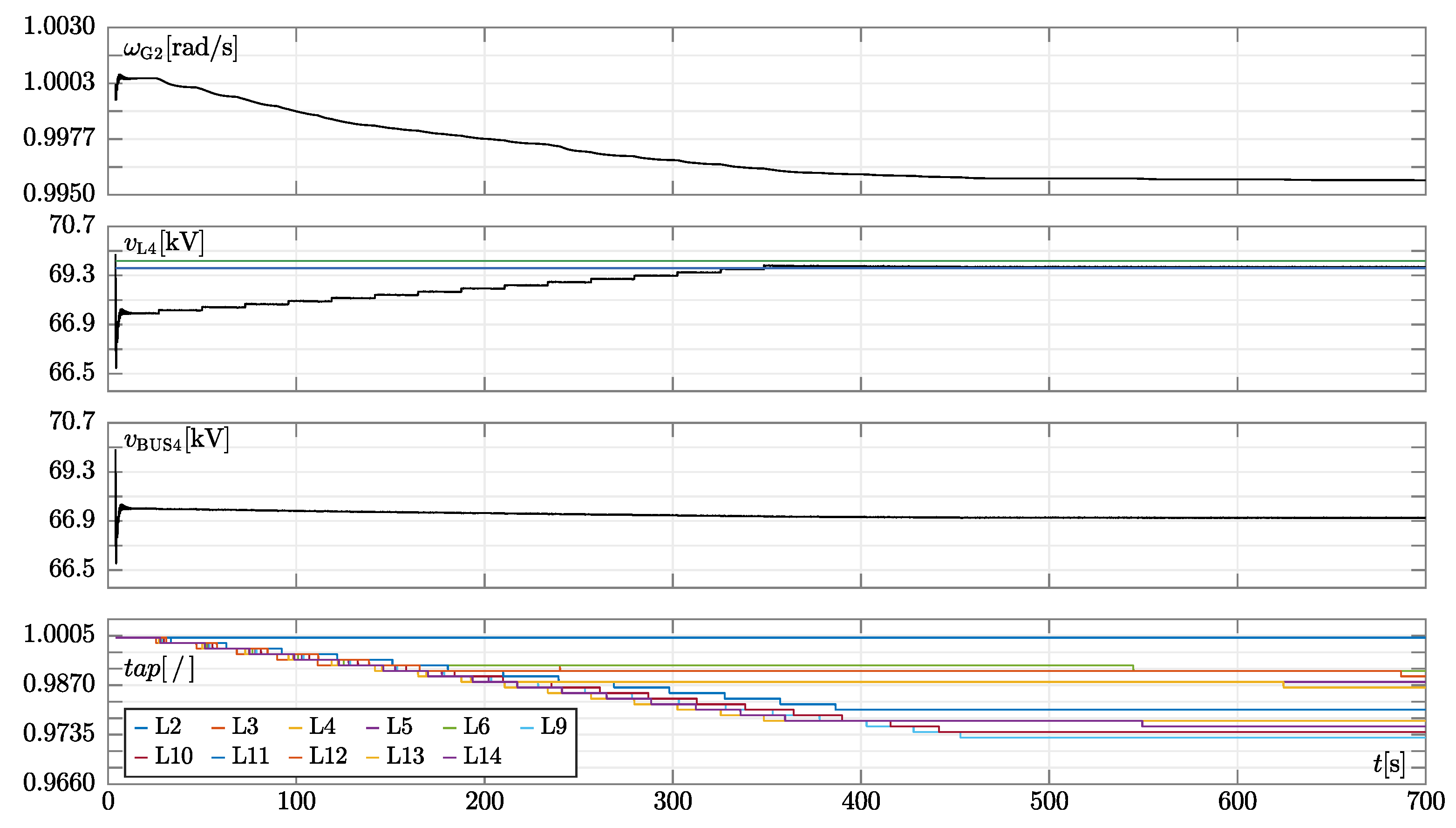
To check the possible onset of an sso we performed a long-lasting transient analysis of the ieee14 benchmark, where at $t=4\mathrm{s}$ the line between bus2 and bus5 was tripped as before (compared to other case studies, the time of occurrence of the disturbance was reduced to minimise the simulation effort, since the simulation of detailed mmc models is more cpu time consuming). We started with the same set-points used to compute impedances of mmcs. As previously mentioned, instabilities could be due to an unstable rlc resonator and/or ssos. To confine the onset of possible unstable modes to only sso, we did not consider any dynamics of passive elements (i.e., $L=0$).

As it can be seen from the results in Figure 11, oltcs intervene once again to restore load voltages and, thus, power. The voltage at bus5, where the potentially critical mmc1 is connected, is also restored. Any stability problem was not evidenced at the current power level, as it was too low to trigger ssos.

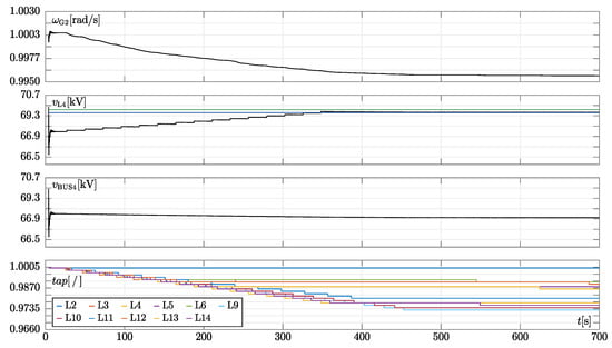
Figure 11. Simulation results of the modified ieee14 test system shown in Figure 6 when the line between bus2 and bus5 is tripped at $4\mathrm{s}$. In this case, an accurate mmc model is used for both mmc1 and mmc2. Constant impedance loads behind oltcs and non-dynamic line and transformer models are used. The traces in each panel have the same meaning as those in Figure 3.

After having restored and stabilised bus voltages inside the dead-bands of oltc, we started to slowly increase the power set point of the p/q type mmc1. The slow increase of power is done to allow the system to adapt to the new working condition and to adequately identify the power level at which it becomes unstable. The corresponding results of the transient stability analysis are reported in Figure 12.

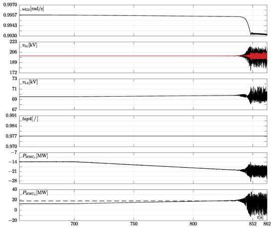
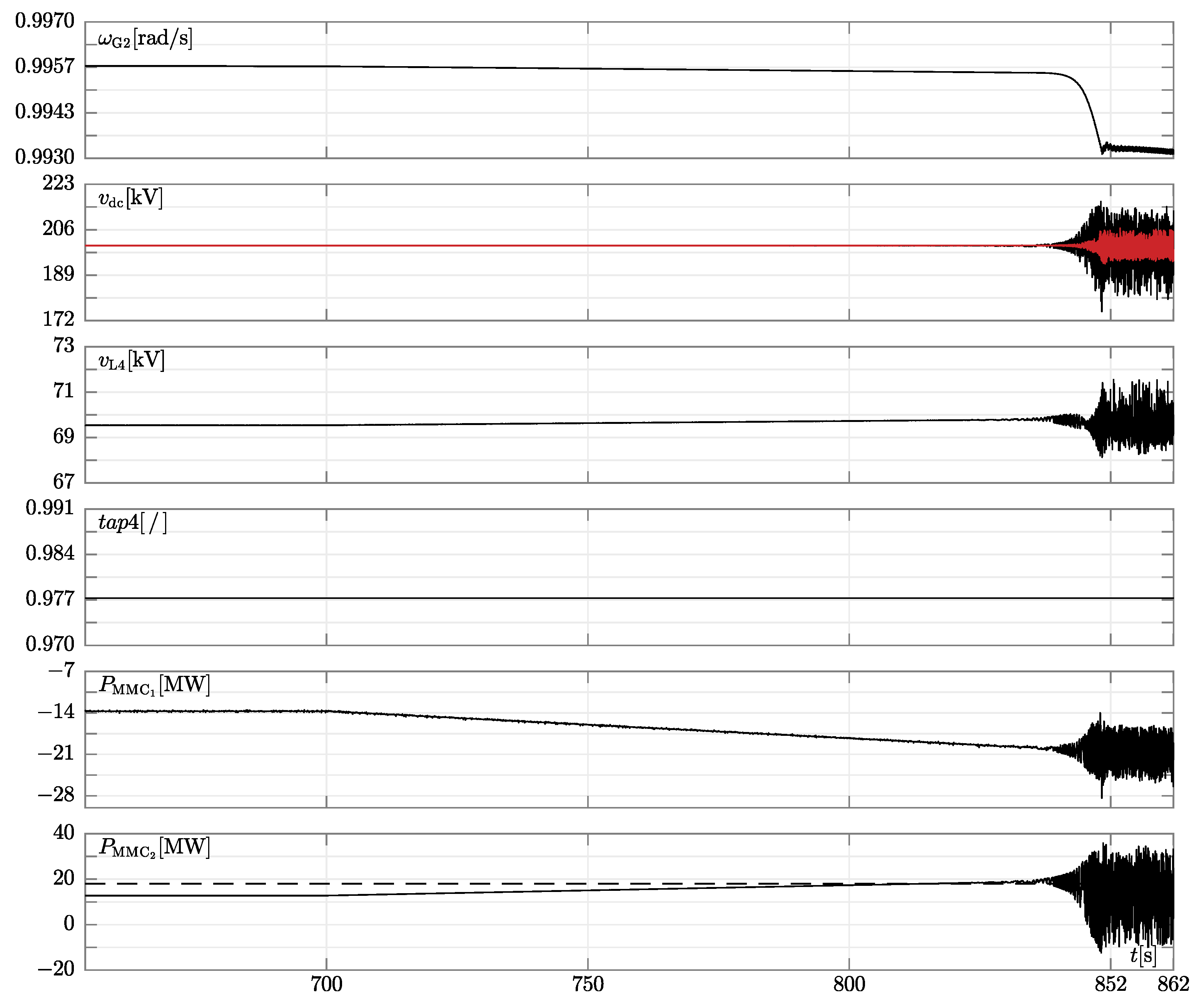
Figure 12. Simulation results of the modified ieee14 test system shown in Figure 6 when the line between bus2 and bus5 is tripped at $4\mathrm{s}$. The results shown in these plots are a sequel to those in Figure 11: mmc, load, line, and transformer models used are the same. In this case, the active power set-point of mmc1 changes linearly from $700\mathrm{s}$ and system instability arises when the power goes above $17\mathrm{M}\mathrm{W}$. Second panel from the top: pole-to-ground voltage of mmc1 (black trace) and mmc2 (red trace). Fifth and last panel from the top: active power exchange of mmc1 and mmc2. The dashed line in the last panels denotes the active power reference value above which the system becomes unstable (i.e., $17\mathrm{M}\mathrm{W}$). The traces in the other panels have the same meaning as those in Figure 3.

When the power goes above $17\mathrm{M}\mathrm{W}$ (which is well below the final $60.7\mathrm{M}\mathrm{W}$ target), instability occurs as shown by the divergence in the pole-to-ground voltage and power exchange of the mmcs. Since in this transient stability analysis we did not use dynamic models of lines and transformers, this unstable behaviour can only be ascribed to ssos [51].

A possible countermeasure to prevent ssos from originating (and, thus, damping the unstable electro-mechanical modes) consists of increasing the damping parameter of the synchronous generators and condensers. To validate this statement, we repeated the simulation and artificially increased the damping parameter of all the synchronous generators and condensers to 10.

The results obtained in this case are shown in Figure 13.

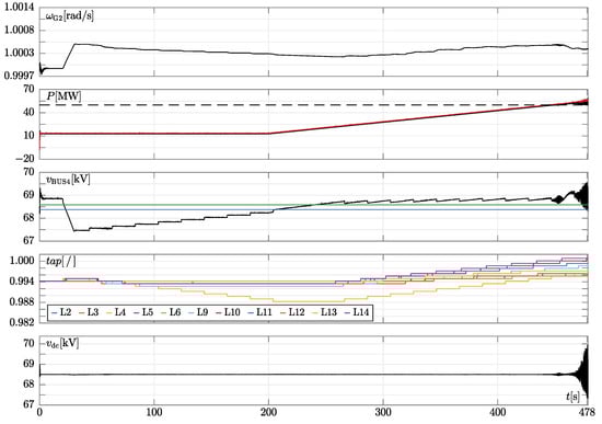
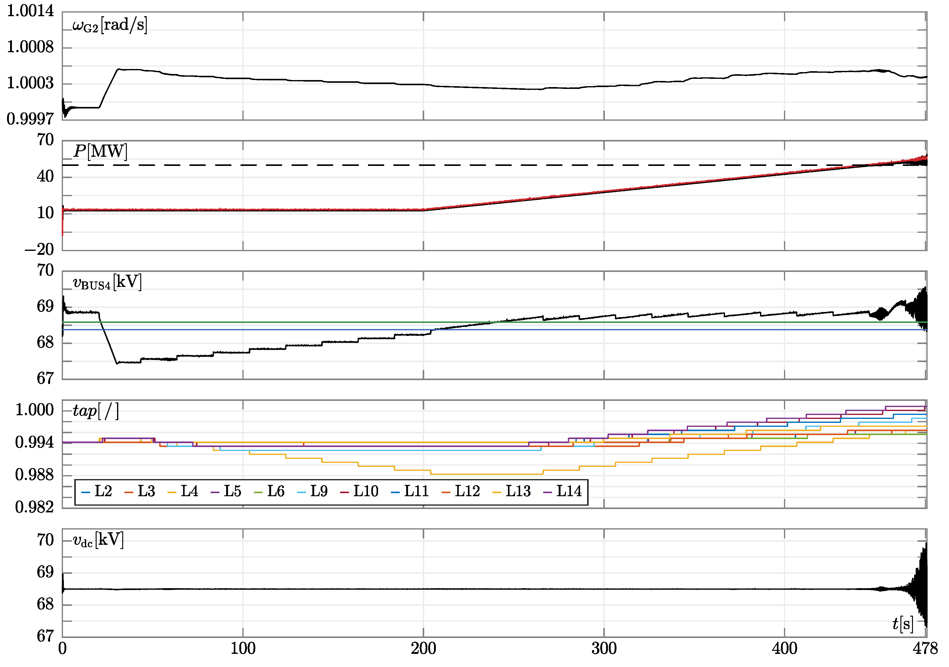
Figure 13. Simulation results of the modified ieee14 test system shown in Figure 6 when the line between bus2 and bus5 is tripped at $4\mathrm{s}$ and the damping of all synchronous generators and condensers were set to 10. mmc, load, line, and transformer models used are the same as those of previous simulations. Analogously to Figure 12, the active power set-point of mmc1 changes linearly. The second panel from the top: active power exchange of mmc1 (black trace) and mmc2 (red trace). The dashed line denotes the active power reference value above which the system becomes unstable (i.e., $50\mathrm{M}\mathrm{W}$). Last panel: pole-to-pole voltage of mmc1. The traces in the other panels have the same meaning as those in Figure 3.

We see that during power ramp-up of mmc1 (and thus of mmc2) the oltc at bus4 increases its transformer ratio to bring voltage inside the dead band. Voltage increases since power voltage drops of transmission lines lower. The other oltcs perform in a similar way. We see that stability is ensured up to $P=50\mathrm{M}\mathrm{W}$. If the power absorbed by the sending converter is further increased instability occurs, which means that increasing damping is effective only to a limited extent in preventing ssos.

As a last comment, it is worth pointing out that all of these features would not be visible by adopting constant power loads. Moreover, also the model of the passive elements play a relevant role: indeed, if dynamic line and transformer representations were used, other instabilities than ssos (i.e., attributable to an unstable rlc resonator) might arise.

5. Conclusions

Our analyses highlight that the well-established phasor analysis and single-phase equivalent models of power elements successfully used so far to study power system stability are no longer valid due to the ever-increasing penetration of ibrs (i.e., generation, load and energy conversion systems interfaced with the grid through power electronic converters). The simulated case studies suggest that a paradigm shift is necessary to study accurately modern electricity networks. In principle, detailed electro-magnetic transient (emt) models of the entire system should be used to ensure accurate results are as adherent as possible to the real grid under study. However, this numerical approach is still impractical today, even on the most powerful computers, due to the scale and complexity of modern power grids, which require solving dynamic models composed of a very large number of equations and unknowns.

We believe that a more promising approach in this regard consists in suitably mixing single-phase dynamic models and accurate three-phase emt models to perform hybrid phasor-emt numerical analyses, thereby achieving a proper compromise between simulation speed and accuracy [54]. The former could represent non-critical parts of the grids (i.e., conventional power grids), while the latter could account for the critical ones (i.e., those comprising large shares of ibrs). However, the issue of how to efficiently partition the power grid in these two parts is still an open question and requires further analysis from our standpoint. According to our analyses, the coupling between conventional and modern grid elements lead to challenges in studying long-term dynamic stability. For example, despite being stable per se (i.e., their designs are correct and lead to stability if considered on their own), the connection of the ieee14 and dcs1 hvdc benchmarks may lead to an overall unstable power system. In particular, this outcome also depends on the models of loads and passive components adopted, which need careful reconsideration due to the increasing presence of ibrs. This is the main challenge of modern and future ibr-dominated power grids.

References

- Hatziargyriou, N.; Milanović, J.; Rahmann, C.; Ajjarapu, V.; Canizares, C.; Erlich, I.; Hill, D.; Hiskens, I.; Kamwa, I.; Pal, B.; et al. Definition and Classification of Power System Stability—Revisited & Extended. IEEE Trans. Power Syst. 2021, 36, 3271–3281. [Google Scholar] [CrossRef]
- Musca, R.; Gonzalez-Longatt, F.; Gallego Sánchez, C.A. Power System Oscillations with Different Prevalence of Grid-Following and Grid-Forming Converters. Energies 2022, 15, 4273. [Google Scholar] [CrossRef]
- Milanović, J.V.; Yamashita, K.; Martínez Villanueva, S.; Djokic, S.v.; Korunović, L.M. International Industry Practice on Power System Load Modeling. IEEE Trans. Power Syst. 2013, 28, 3038–3046. [Google Scholar] [CrossRef]
- Korunović, L.M.; Milanović, J.V.; Djokic, S.Z.; Yamashita, K.; Villanueva, S.M.; Sterpu, S. Recommended Parameter Values and Ranges of Most Frequently Used Static Load Models. IEEE Trans. Power Syst. 2018, 33, 5923–5934. [Google Scholar] [CrossRef]
- Pasiopoulou, I.; Kontis, E.; Papadopoulos, T.; Papagiannis, G. Effect of load modeling on power system stability studies. Electr. Power Syst. Res. 2022, 207, 107846. [Google Scholar] [CrossRef]
- Overbye, T. Effects of load modelling on analysis of power system voltage stability. Int. J. Electr. Power Energy Syst. 1994, 16, 329–338. [Google Scholar] [CrossRef]
- EL-Shimy, M.; Mostafa, N.; Afandi, A.; Sharaf, A.; Attia, M.A. Impact of load models on the static and dynamic performances of grid-connected wind power plants: A comparative analysis. Math. Comput. Simul. 2018, 149, 91–108. [Google Scholar] [CrossRef]
- Zhang, X.P.; Chen, H. Analysis and selection of transmission line models used in power system transient simulations. Int. J. Electr. Power Energy Syst. 1995, 17, 239–246. [Google Scholar] [CrossRef]
- Milano, F. Power System Modelling and Scripting; Power Systems; Springer: Berlin/Heidelberg, Germany, 2010. [Google Scholar]
- Matevosyan, J.; MacDowell, J.; Miller, N.; Badrzadeh, B.; Ramasubramanian, D.; Isaacs, A.; Quint, R.; Quitmann, E.; Pfeiffer, R.; Urdal, H.; et al. A Future with Inverter-Based Resources: Finding Strength From Traditional Weakness. IEEE Power Energy Mag. 2021, 19, 18–28. [Google Scholar] [CrossRef]
- Franquelo, L.G.; Rodriguez, J.; Leon, J.I.; Kouro, S.; Portillo, R.; Prats, M.A.M. The age of multilevel converters arrives. IEEE Ind. Electron. Mag. 2008, 2, 28–39. [Google Scholar] [CrossRef] [Green Version]
- Lesnicar, A.; Marquardt, R. An innovative modular multilevel converter topology suitable for a wide power range. In Proceedings of the Power Tech Conference Proceedings, Bologna, Italy, 23–26 June 2003; Volume 3, pp. 6–10. [Google Scholar]
- Dekka, A.; Wu, B.; Fuentes, R.L.; Perez, M.; Zargari, N.R. Evolution of topologies, modeling, control schemes, and applications of modular multilevel converters. IEEE J. Emerg. Sel. Top. Power Electron. 2017, 5, 1631–1656. [Google Scholar] [CrossRef]
- Martinez-Rodrigo, F.; Ramirez, D.; Rey-Boue, A.; de Pablo, S.; Herrero-de Lucas, L. Modular Multilevel Converters: Control and Applications. Energies 2017, 10, 1709. [Google Scholar] [CrossRef]
- Glover, J.D.; Sarma, M.S.; Overbye, T.J. Power System Analysis and Design; Brooks/Cole Publishing Co.: Pacific Grove, CA, USA, 2001. [Google Scholar]
- Kundur, P. Power System Stability and Control; McGraw-Hill: New York, NY, USA, 1994. [Google Scholar]
- Van Cutsem, R.; Papangelis, L. Description, Modeling and Simulation Results of a Test System for Voltage Stability Analysis; University of Liège: Liège, Belgium, 2013; pp. 1–16. [Google Scholar]
- Milano, F. Hybrid Control Model of Under Load Tap Changers. IEEE Trans. Power Deliv. 2011, 26, 2837–2844. [Google Scholar] [CrossRef]
- DIgSILENT. PowerFactory User Manual; DIgSILENT GmbH: Gomaringen, Germany, 2020. [Google Scholar]
- Dommel, H.W. Digital Computer Solution of Electromagnetic Transients in Single-and Multiphase Networks. IEEE Trans. Power Appar. Syst. 1969, PAS-88, 388–399. [Google Scholar] [CrossRef]
- Murad, M.A.A.; Mele, F.M.; Milano, F. On the Impact of Stochastic Loads and Wind Generation on Under Load Tap Changers. In Proceedings of the 2018 IEEE Power Energy Society General Meeting (PESGM), Portland, OR, USA, 5–10 August 2018; pp. 1–5. [Google Scholar] [CrossRef]
- Liu, M.; Bizzarri, F.; Brambilla, A.M.; Milano, F. On the Impact of the Dead-Band of Power System Stabilizers and Frequency Regulation on Power System Stability. IEEE Trans. Power Syst. 2019, 34, 3977–3979. [Google Scholar] [CrossRef]
- Fudeh, H.; Ong, C.M. A Simple and Efficient AC-DC Load-Flow Method for Multiterminal DC Systems. IEEE Trans. Power Appar. Syst. 1981, PAS-100, 4389–4396. [Google Scholar] [CrossRef]
- Sanghavi, H.A.; Banerjee, S.K. Load flow analysis of integrated AC-DC power systems. In Proceedings of the Fourth IEEE Region 10 International Conference TENCON, Bombay, India, 22–24 November 1989; pp. 746–751. [Google Scholar]
- Feng, W.; Yuan, C.; Shi, Q.; Dai, R.; Liu, G.; Wang, Z.; Li, F. Using virtual buses and optimal multipliers to converge the sequential AC/DC power flow under high load cases. Electr. Power Syst. Res. 2019, 177, 106015. [Google Scholar] [CrossRef]
- del Giudice, D.; Brambilla, A.; Linaro, D.; Bizzarri, F. Modular Multilevel Converter Impedance Computation Based on Periodic Small-Signal Analysis and Vector Fitting. IEEE Trans. Circuits Syst. I Regul. Pap. 2022, 69, 1832–1842. [Google Scholar] [CrossRef]
- Cigré Working Group B4.57. Guide for the Development of Models for HVDC Converters in a HVDC Grid; CIGRÉ (WG Brochure No. 604); CIGRÉ: Paris, France, 2014. [Google Scholar]
- Wang, S.; Bao, D.; Gontijo, G.; Chaudhary, S.; Teodorescu, R. Modeling and Mitigation Control of the Submodule-Capacitor Voltage Ripple of a Modular Multilevel Converter under Unbalanced Grid Conditions. Energies 2021, 14, 651. [Google Scholar] [CrossRef]
- Wu, H.; Wang, X. Dynamic Impact of Zero-Sequence Circulating Current on Modular Multilevel Converters: Complex-Valued AC Impedance Modeling and Analysis. IEEE J. Emerg. Sel. Top. Power Electron. 2020, 8, 1947–1963. [Google Scholar] [CrossRef]
- Peralta, J.; Saad, H.; Dennetiere, S.; Mahseredjian, J.; Nguefeu, S. Detailed and Averaged Models for a 401-Level MMC–HVDC System. IEEE Trans. Power Deliv. 2012, 27, 1501–1508. [Google Scholar] [CrossRef]
- Khan, S.; Tedeschi, E. Modeling of MMC for Fast and Accurate Simulation of Electromagnetic Transients: A Review. Energies 2017, 10, 1161. [Google Scholar] [CrossRef]
- del Giudice, D.; Brambilla, A.; Linaro, D.; Bizzarri, F. Isomorphic Circuit Clustering for Fast and Accurate Electromagnetic Transient Simulations of MMCs. IEEE Trans. Energy Convers. 2022, 37, 800–810. [Google Scholar] [CrossRef]
- Xu, J.; Ding, H.; Fan, S.; Gole, A.M.; Zhao, C.; Xiong, Y. Ultra-fast electromagnetic transient model of the modular multilevel converter for HVDC studies. In Proceedings of the 12th IET International Conference on AC and DC Power Transmission (ACDC 2016), Beijing, China, 28–29 May 2016; pp. 1–9. [Google Scholar] [CrossRef]
- Meng, X.; Han, J.; Pfannschmidt, J.; Wang, L.; Li, W.; Zhang, F.; Belanger, J. Combining Detailed Equivalent Model with Switching-Function-Based Average Value Model for Fast and Accurate Simulation of MMCs. IEEE Trans. Energy Convers. 2020, 35, 484–496. [Google Scholar] [CrossRef]
- Song, G.; Wang, T.; Huang, X.; Zhang, C. An improved averaged value model of MMC-HVDC for power system faults simulation. Int. J. Electr. Power Energy Syst. 2019, 110, 223–231. [Google Scholar] [CrossRef]
- Freytes, J.; Papangelis, L.; Saad, H.; Rault, P.; Van Cutsem, T.; Guillaud, X. On the modeling of MMC for use in large scale dynamic simulations. In Proceedings of the 2016 Power Systems Computation Conference (PSCC), Genova, Italy, 20–24 June 2016; pp. 1–7. [Google Scholar] [CrossRef]
- Zhu, S.; Liu, K.; Qin, L.; Ran, X.; Li, Y.; Huai, Q.; Liao, X.; Zhang, J. Reduced-Order Dynamic Model of Modular Multilevel Converter in Long Time Scale and Its Application in Power System Low-Frequency Oscillation Analysis. IEEE Trans. Power Deliv. 2019, 34, 2110–2122. [Google Scholar] [CrossRef]
- Guo, D.; Rahman, M.H.; Ased, G.P.; Xu, L.; Emhemed, A.; Burt, G.; Audichya, Y. Detailed quantitative comparison of half-bridge modular multilevel converter modelling methods. J. Eng. 2019, 2019, 1292–1298. [Google Scholar] [CrossRef]
- Bizzarri, F.; Giudice, D.D.; Linaro, D.; Brambilla, A. Partitioning-Based Unified Power Flow Algorithm for Mixed MTDC/AC Power Systems. IEEE Trans. Power Syst. 2021, 36, 3406–3415. [Google Scholar] [CrossRef]
- Beerten, J.; Belmans, R. Development of an open source power flow software for high voltage direct current grids and hybrid AC/DC systems: MATACDC. IET Gener. Transm. Distrib. 2015, 9, 966–974. [Google Scholar] [CrossRef]
- Aik, D.; Andersson, G. Use of participation factors in modal voltage stability analysis of multi-infeed HVDC systems. IEEE Trans. Power Deliv. 1998, 13, 203–211. [Google Scholar] [CrossRef]
- Abed, E.H.; Lindsay, D.; Hashlamoun, W.A. On participation factors for linear systems. Automatica 2000, 36, 1489–1496. [Google Scholar] [CrossRef]
- Perez-arriaga, I.J.; Verghese, G.C.; Schweppe, F.C. Selective Modal Analysis with Applications to Electric Power Systems, PART I: Heuristic Introduction. IEEE Trans. Power Appar. Syst. 1982, PAS-101, 3117–3125. [Google Scholar] [CrossRef]
- del Giudice, D.; Bizzarri, F.; Linaro, D.; Brambilla, A. Stability Analysis of MMC/MTDC Systems Considering DC-Link Dynamics. In Proceedings of the 2021 IEEE International Symposium on Circuits and Systems (ISCAS), Daegu, Korea, 22–28 May 2021; pp. 1–5. [Google Scholar] [CrossRef]
- Wu, H.; Wang, X.; Kocewiak, L.H. Impedance-Based Stability Analysis of Voltage-Controlled MMCs Feeding Linear AC Systems. IEEE J. Emerg. Sel. Top. Power Electron. 2020, 8, 4060–4074. [Google Scholar] [CrossRef]
- Zhu, S.; Qin, L.; Liu, K.; Ji, K.; Li, Y.; Huai, Q.; Liao, X.; Yang, S. Impedance Modeling of Modular Multilevel Converter in D-Q and Modified Sequence Domains. IEEE J. Emerg. Sel. Top. Power Electron. 2022, 10, 4361–4382. [Google Scholar] [CrossRef]
- Zhu, S.; Liu, P.; Liao, X.; Qin, L.; Huai, Q.; Xu, Y.; Li, Y.; Wang, F. D-Q Frame Impedance Modeling of Modular Multilevel Converter and Its Application in High-Frequency Resonance Analysis. IEEE Trans. Power Deliv. 2021, 36, 1517–1530. [Google Scholar] [CrossRef]
- Linaro, D.; del Giudice, D.; Bizzarri, F.; Brambilla, A. PanSuite: A free simulation environment for the analysis of hybrid electrical power systems. Electr. Power Syst. Res. 2022, 212, 108354. [Google Scholar] [CrossRef]
- Bizzarri, F.; Brambilla, A. PAN and MPanSuite: Simulation Vehicles Towards the Analysis and Design of Heterogeneous Mixed Electrical Systems. In Proceedings of the NGCAS, Genova, Italy, 6–9 September 2017; pp. 1–4. [Google Scholar]
- Zong, H.; Zhang, C.; Lyu, J.; Cai, X.; Molinas, M.; Rao, F. Generalized MIMO Sequence Impedance Modeling and Stability Analysis of MMC-HVDC with Wind Farm Considering Frequency Couplings. IEEE Access 2020, 8, 55602–55618. [Google Scholar] [CrossRef]
- Damas, R.N.; Son, Y.; Yoon, M.; Kim, S.Y.; Choi, S. Subsynchronous Oscillation and Advanced Analysis: A Review. IEEE Access 2020, 8, 224020–224032. [Google Scholar] [CrossRef]
- Ghaffarzadeh, H.; Mehrizi-Sani, A. Review of control techniques for wind energy systems. Energies 2020, 13, 6666. [Google Scholar] [CrossRef]
- He, C.; Sun, D.; Song, L.; Ma, L. Analysis of subsynchronous resonance characteristics and influence factors in a series compensated transmission system. Energies 2019, 12, 3282. [Google Scholar] [CrossRef]
- Linaro, D.; del Giudice, D.; Brambilla, A.; Bizzarri, F. Application of Envelope-Following Techniques to the Simulation of Hybrid Power Systems. IEEE Trans. Circuits Syst. I Regul. Pap. 2022, 69, 1800–1810. [Google Scholar] [CrossRef]
Publisher’s Note: MDPI stays neutral with regard to jurisdictional claims in published maps and institutional affiliations. |
© 2022 by the authors. Licensee MDPI, Basel, Switzerland. This article is an open access article distributed under the terms and conditions of the Creative Commons Attribution (CC BY) license (https://creativecommons.org/licenses/by/4.0/).