Abstract
The development of the Light Detection and Ranging (LIDAR) technology has enabled wider options for wind turbine control, in particular regarding disturbance rejection. The LIDAR measurements provide a spatial, preview wind information, based on which the controller has a better chance to cope with the wind disturbance before it affects the turbine operation. In this paper, a model predictive controller for above-rated wind turbine control was developed with the use of pseudo-LIDAR wind measurements data. A predictive control algorithm was developed based on a linearised wind turbine model, in which the disturbance from the incoming wind was computed by the LIDAR simulator. The optimal control action was applied to the nonlinear turbine model. The developed controller was compared with the baseline control and a previously developed LIDAR-assisted control combining a feedback-and-feedforward design. Our simulation studies on a 5 MW nonlinear wind turbine model, under different wind conditions, demonstrated that the developed LIDAR-based predictive control achieved improved performance in the presence of small variations in the out-of-plane rotor torque and fore-aft tower acceleration, as well as a smoother generator speed regulation and satisfied pitch activity control constraints.
1. Introduction
With the increased demand on effective power generation and reduced production cost, large-scale wind turbines have become popular in the modern wind industry [1]. Large wind turbines have higher energy capture capacities and, therefore, a higher requirement of power conversion efficiency. Components in large turbines are often made of flexible materials. However, the turbulent wind conditions experienced by large turbines can cause serious fatigue damages to the turbines and require load reduction control, especially for the above-rated operations.
Conventional wind turbine control systems often use a feedback control scheme, in which proportional–integral (PI) or proportional–integral–derivative (PID) controllers are designed in response to sensor signals such as the generator speed and/or the tower head acceleration [2,3,4,5]. The PI and PID control designs can achieve a satisfactory energy capture performance. In addition, load reduction strategies have been developed, including the damping of resonances on the drivetrain and tower, which results in load reduction at specific frequencies [6,7,8], and the alleviation of rotor asymmetrical loads through individual pitch control (IPC) or individual blade control (IBC) [9,10,11]. There is an inherent delay problem with feedback control designs, that is, the controller can only respond to changes measured and transmitted via feedback. This means the controller can only make responses after the turbine has been affected by the turbulent wind. New methods need to be developed to reduce the impact of such delays in standard feedback control.
A Light Detection and Ranging (LIDAR) equipment mounted on the turbine nacelle or hub functions by emitting laser beams to scan the approaching wind field and thus obtain a spatial preview wind information that could be utilised to enhance the wind turbine control. Various LIDAR-assisted wind turbine control designs have been developed including the combined feedback/feedforward control, the preview control and the model predictive control (MPC).
The combined feedback/feedforward control, called FB-FF in this paper, was proposed for LIDAR-assisted control [12,13]; in it, a feedforward channel is introduced to compensate the wind disturbance by using the LIDAR-measured wind speed. In a standard FB-FF control scheme, an inversion of the wind turbine model is required, which causes unstable dynamics due to the right-half-plane zeros in the model. Therefore, a stable approximation of the model inversion is needed. A non-causal series expansion method for the stable approximation was developed in [14]. Variations of FB-FF control designs were developed. In [15], a preview control scheme using an H-infinity method was developed based on LIDAR wind measurements. An adaptive expansion of the FB-FF control was developed in [16], where the controller was designed to deal with the highly non-linear turbine dynamics using the filtered-x recursive least-square algorithm. In [17], a multivariable FB-FF controller was designed for the transition between partial and full load operations and assisted both the generator torque control and the blade pitch control of the baseline feedback controller.
While most of the designs were implemented through generator torque and blade pitch control, LIDAR-based augmentations on yaw control for energy capture and/or load reduction purposes were also investigated [18,19,20].
MPC has been used in wind turbine control for a range of operational and economical objectives, leading to the scheduled MPC for full operation modes [21], economic MPC strategies [22,23], and the MPC with aero-elastically tailored blades [24]. LIDAR-based wind turbine MPC designs were also presented in various studies with the use of linear and non-linear methods. In [25], an MPC design with a particular focus on rotor speed constraints was proposed, assisted by LIDAR-measured wind speed information. In [26], a LIDAR-based MPC for wind turbine was developed, where the computational cost of the controller was taken into consideration to assess the control performance. A non-linear MPC design using LIDAR was proposed in [27], in which the generator torque and the blade pitch angle were controlled simultaneously.
In the MPC of wind turbine control, the model prediction is influenced by the wind speed. LIDAR measurements provide preview information of the incoming wind speed, which can be processed to enhance MPC strategies. The potential of integrating LIDAR wind information into MPC needs to be further explored for industrial-scale turbines. In this work, we aimed to develop a LIDAR-based MPC for the above-rated turbine control and make a comparison with the baseline control and the previously developed LIDAR-assisted FB-FF design. The remaining part of the paper is organised as follows. Section 2 describes the design and simulation environments including the pseudo-LIDAR data generation, the wind turbine model and the baseline controller. The proposed LIDAR-based MPC controller design is presented in Section 3. Simulation studies and results are discussed in Section 4. Finally, the conclusions are reported in Section 5.
2. Design and Simulation Framework
In this section, key elements of the LIDAR-assisted wind turbine modelling and baseline control are presented.
2.1. LIDAR Data Generation
The pseudo-LIDAR data used in this work were generated from Bladed [28]. The original data were used to construct a turbulent wind field. The modelling details were presented in our previous publication [29]. The generated wind field had three directional components. By re-selecting the wind incoming direction and employing the designed sampling strategy, the pseudo-LIDAR wind measurements on a scanning plane could be derived. The wind field was then converted into a rotor effective wind speed, for control design purposes, by averaging the wind speed points over the rotor plane. This data generation process is called LIDAR simulator in the following sections.
2.2. Wind Turbine Model
2.2.1. Model Configuration
The 5 MW Supergen Exemplar wind turbine model [4] was used in this work. The model configuration is shown in Figure 1. It contains the necessary components for a modern MW-scale wind turbine, some of which are briefed in the following subsections. More details can be found in [4,30,31]. The model describes a variable-speed pitch-regulated wind turbine. During below-rated operations, where the wind speed is between the cut-in speed and the rated speed, the generator speed of the wind turbine can be regulated to achieve the maximum energy capture. During above-rated operations, where the wind speed is between the rated and the cut-out level, the pitch angle of the blades can be regulated to maintain the rated power output. The basic parameters of the wind turbine model are shown in Table 1.
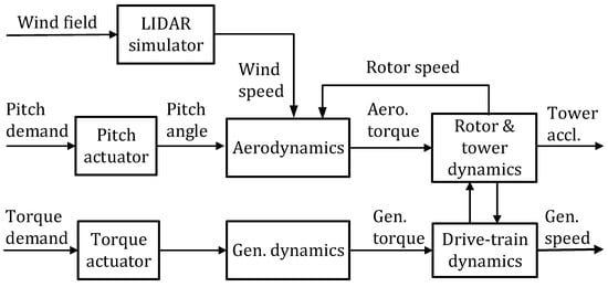
Figure 1.
Wind turbine model structure.

Table 1.
Main parameters of the 5 MW Supergen exemplar wind turbine model.
The nonlinearities of the wind turbine dynamics mainly derive from the nonlinear aerodynamics caused by the interaction between the wind field and the wind turbine rotor. Some details about the nonlinear relationships for the aero-rotor dynamics and the corresponding tower and drivetrain dynamics are presented in the following sections.
2.2.2. Aero-Rotor Dynamics
The aero-rotor dynamics defines the motions of the rotor in the out-of-plane and in-plane directions. Here, the plane denotes the rotor plane of the wind turbine. The dynamics are expressed by Equations (1) and (2).
where
- θR and ΦR are the displacements of the rotor in the in-plane and out-of-plane directions, respectively;
- θH is the rotational displacement of the hub;
- and are the in-plane and out-of-plane rotor speeds;
- and are the in-plane and out-of-plane rotor accelerations;
- Qin and Qout are the in-plane and out-of-plane aerodynamic torques on the rotor;
- J, Jt and Jc are the rotor inertia, tower fore-aft inertia and rotor/tower cross coupling inertia;
- Ke, Kf and Kt are the blade edge-wise stiffness, flap-wise stiffness and tower fore-aft stiffness;
- Bt is the tower fore-aft damping moment;
- β is the blade pitch angle.
2.2.3. Tower Dynamics
The tower dynamics defines the motions of the tower in the fore-aft and side-to-side directions, as shown in Equations (3) and (4).
where
- θT and ΦT are the displacements of the tower in the side-to-side and fore-aft directions;
- and are the side-to-side and fore-aft tower speeds;
- and are the side-to-side and fore-aft tower accelerations;
- Jts, Kts and Bts are the tower side-to-side inertia, stiffness and damping moment;
- N is the gearbox ratio, TLs is the gearbox torque at the low-speed shaft.
2.2.4. Drive Train Dynamics
The drivetrain model consisted of the low-speed shaft, the gearbox, the high-speed shaft and the power generation unit. This model was connected to the aero-rotor dynamics block and produced the generator speed, and hence, the power output of the whole wind turbine model. The generator speed output is modelled in (5). See [30,31] for details.
Here, is the rotational displacement of the generator, and are the generator speed and acceleration. IHs is the sum of the generator inertia and the high-speed shaft inertia, THs is the gearbox torque at the high-speed shaft, TG is the generator torque, and is the high-speed shaft damping.
2.3. Linearised Model
The model described in Section 2.2 is a high-dimensional and nonlinear model, which was linearised at specific operating points for controller design.
The linearised and reduced-order model is in continuous-time, state–space format. The following 12 states are included in this model.
- (1).
- In-plane displacement of the rotor, θR
- (2).
- Out-of-plane displacement of the rotor, ΦR
- (3).
- In-plane speed of the rotor,
- (4).
- Out-of-plane speed of the rotor,
- (5).
- Fore-aft displacement of the tower, ΦT
- (6).
- Side-to-side displacement of the tower, θT
- (7).
- Fore-aft speed of the tower,
- (8).
- Side-to-side speed of the tower,
- (9).
- Generator speed,
- (10).
- Hub speed,
- (11).
- Equivalent low- and high-speed shaft displacement
- (12).
- Equivalent low- and high-speed shaft speed
For a full-envelope wind turbine control, the inputs include the torque demand and the pitch demand, and the outputs are the generator speed and the tower fore-aft acceleration. For the above-rated control with pitch regulation, the control input is the pitch demand, and the output is the generator speed; therefore, an SISO system. In this work, the continuous-time state–space model was further discretised for controller design.
2.4. Baseline Controller Description
The baseline control system of the 5 MW wind turbine model was developed to cover the full-range turbine operations [4]. The below-rated generator torque controller and the above-rated blade pitch controller were designed separately. For the control, a global gain-scheduling strategy was developed to address the changes in turbine dynamics due to wind speed variations. The switching between below-rated control and above-rated control and the switching between the first- and second- constant speed regions and the maximum tracking region in the below-rated control were designed with several internal indicators calculated by the model. Two additional filters, i.e., the tower filter and the drivetrain filter, were designed to damp the resonances on the tower base and the drivetrain components at specific frequencies. This gain-scheduling baseline feedback control system achieved satisfactory control performances for full envelope turbine operations.
3. Model Predictive Controller Design
3.1. Control System Configuration
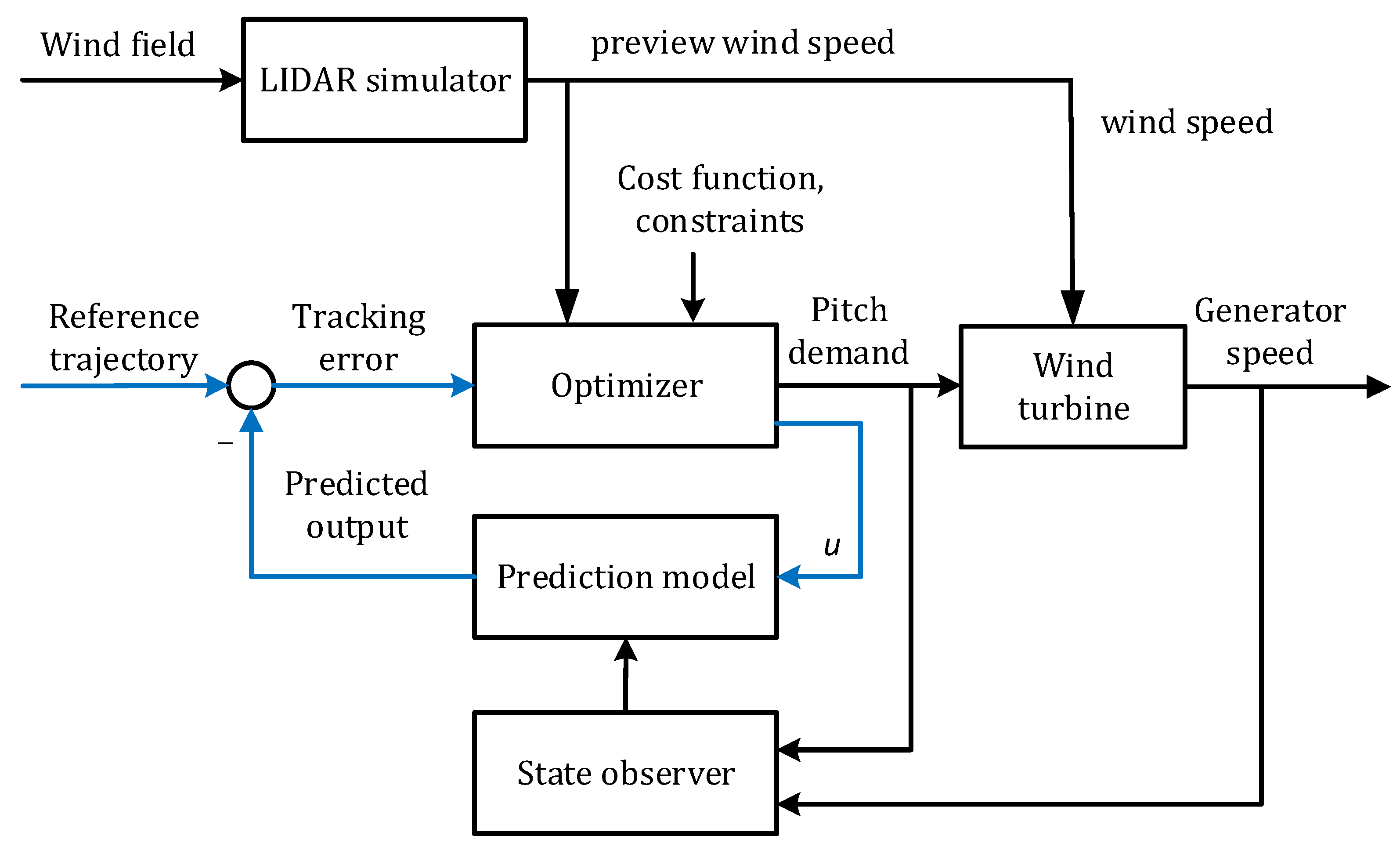
In this section, a predictive control algorithm was developed for the 5 MW exemplar wind turbine during above-rated operations. The structure of the control scheme is shown in Figure 2. Here, the preview wind speed generated by the LIDAR simulator was used in the MPC design. The MPC algorithm was implemented based on the linearised state–space model. The control action computed by MPC was applied to the nonlinear wind turbine model. A state observer was used to update the states of the model. This is helpful when a linearised model is used for the controller design in a nonlinear system.
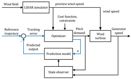
Figure 2.
MPC control structure.
3.2. Basic MPC Algorithm
The wind turbine model is presented in a general discrete-time, state-space form as
where x is the state vector consisting of the 12 states, u is the control input (pitch demand), y is the model output (generator speed). The disturbance term d is from the incoming wind and can be computed from the LIDAR simulator. k is the time instant, and , , are the parameter matrices.
With the model in (6), the one-step ahead output can be calculated. The output predictions within a time range of p steps, which is known as the prediction horizon, can then be derived.
The objective function to be minimised is
At time k, is the tracking error, is the control increment, R is the weighting factor for control input, which is constant in this design. l is the control horizon, p is the prediction horizon.
The control input is computed by minimising the objective function subject to constraints, i.e.,
is the vector of the control input over the control horizon, and are the lower and upper bounds for , and are the lower and upper bounds for . In this work, an interior-point method was employed to solve the optimisation problem in (8), with the embedded function quadprog() in Matlab [32]. The method is suitable to handle quadratic programming problems in fast speed and with low memory usage.
4. Simulation Studies
4.1. Simulation Setting
In this section, the proposed LIDAR-based MPC design was simulated on the nonlinear 5 MW Supergen Exemplar wind turbine model. The MPC controller was compared with two previously developed controllers, one being the baseline control, and the other the LIDAR-assisted FB-FF control described in [29].
Three wind speed sequences were generated by the LIDAR simulator with the assumption of perfect preview. All had a mean value of 18 m/s. The first wind speed had a turbulence intensity of 5%, following the IEC standard 61400, which represents a typical above-rated environment in which the wind speed variations are relatively small, and hence the turbine operating conditions are around the operating point obtained at the mean wind speed. The second wind speed series was generated with a turbulence intensity of 10% to assess the control performance under a larger turbulence intensity. The third wind speed sequence had a turbulence intensity of 15%, because of which the wind speed varied between 13 and 23 m/s. A simulation with such a large turbulence intensity can be used to examine the MPC performance covering almost the full above-rated operational region. The three wind speed time profiles are shown in Figure 3.
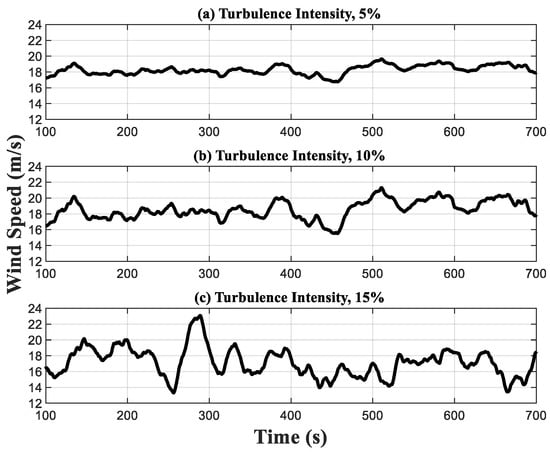
Figure 3.
Wind speed with a mean value of 18 m/s: (a) turbulence intensity of 5%, (b) turbulence intensity of 10%, (c) turbulence intensity of 15%.
The MPC algorithm settings are shown in Table 2. The sampling time was selected following the system dynamics, the prediction horizon and control horizons were tuned by experience and trial and error. The weighting factor was adjusted according to the simulations. The constraints on pitch angle and pitching rate were set up following turbine operation guidance.
Table 2.
MPC parameters.
Comparisons were made concerning power generation, load reduction and pitch activities. The load reduction performance was assessed using the out-of-plane aerodynamic torque on the rotor and the tower fore-aft acceleration. The controlled generator speed was used to reflect the power generation performance, and the blade pitching rate was calculated to compare the control activities.
4.2. Wind Speed with 5% Turbulence Intensity
The simulation results are depicted in Figure 4, Figure 5, Figure 6 and Figure 7, where the load control performance and the pitch activities are presented in both time domain and frequency domain. In all the comparisons including the three controllers, the black dotted line indicates the baseline control, the blue dashed line the LIDAR FB-FF control, and the red solid line the LIDAR MPC. The standard deviation (std) of each time series and its percentage change with respect to the baseline control std are listed in Table 3.
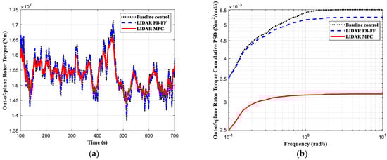
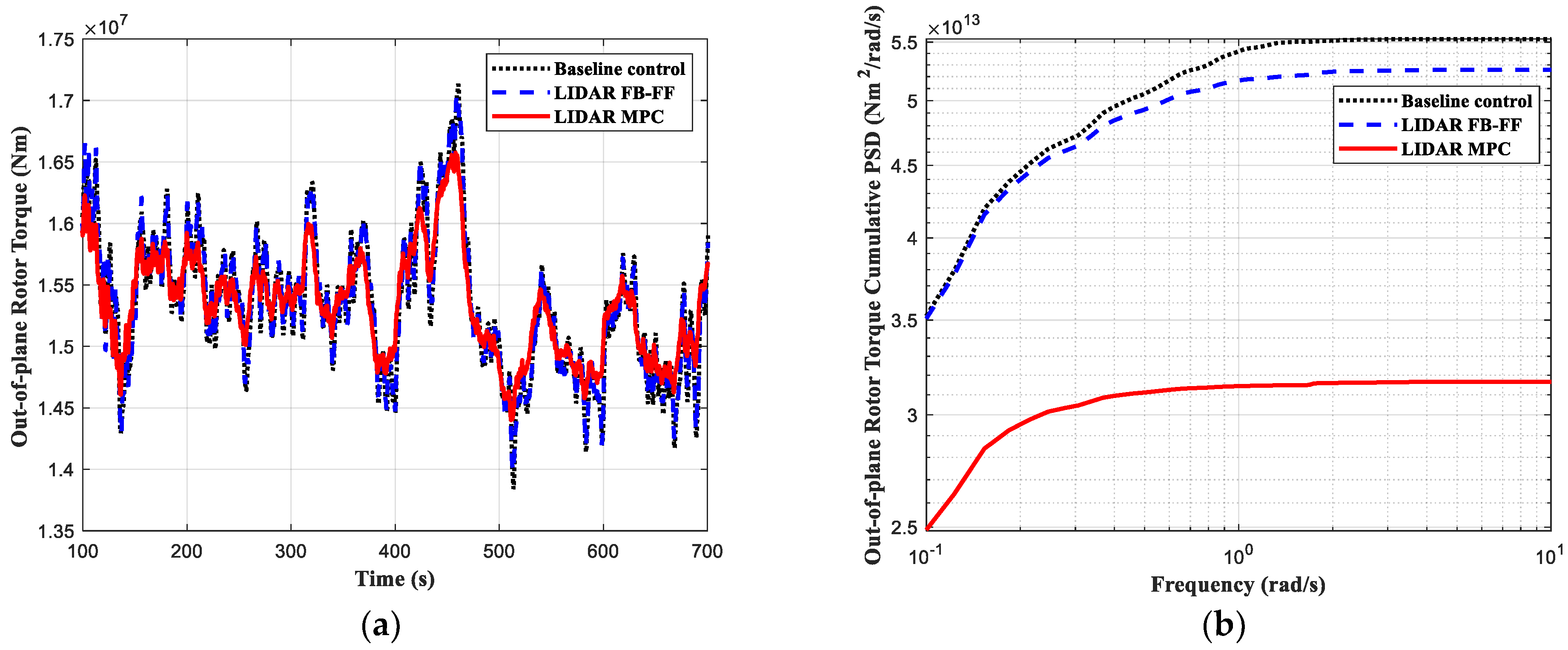
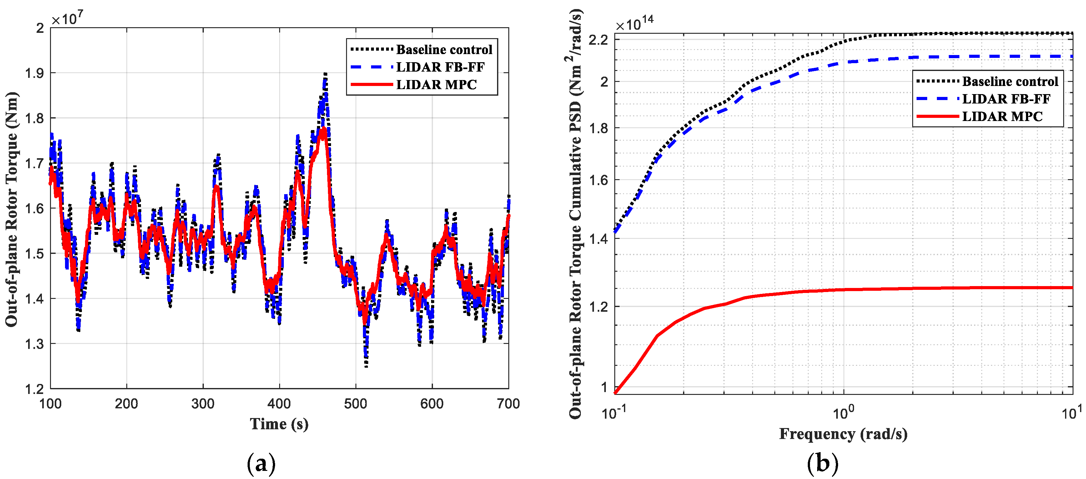
Figure 4.
Out-of-plane rotor torque: (a) time profiles; (b) cumulative PSD (for wind speed with 5% turbulence intensity).
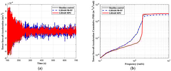
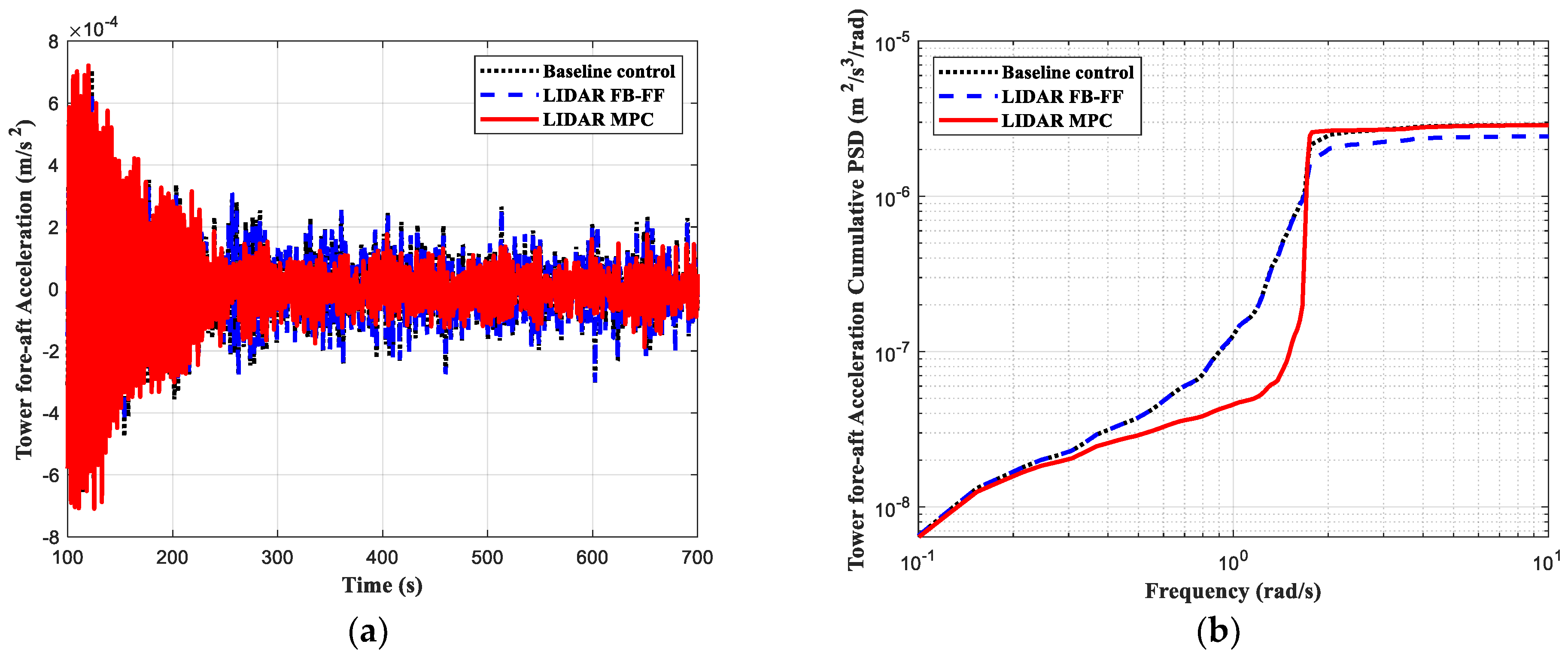
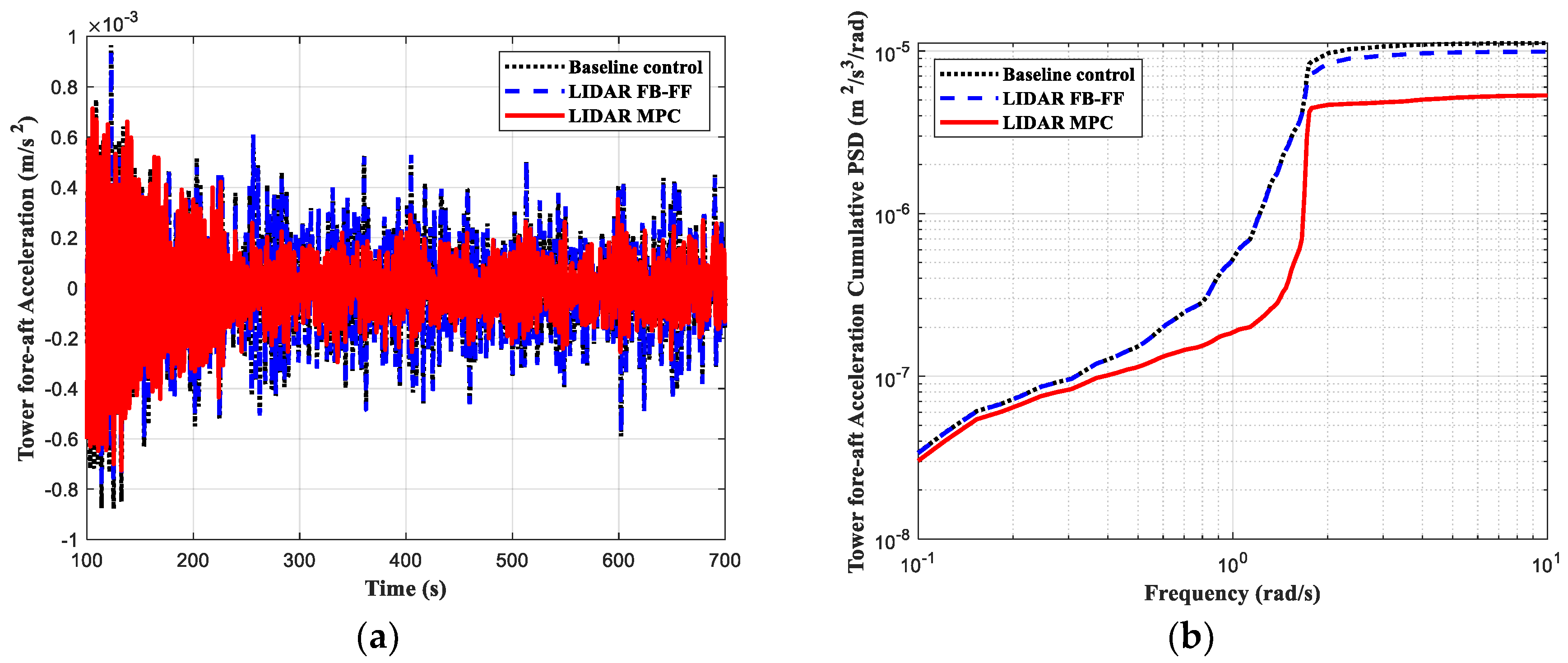
Figure 5.
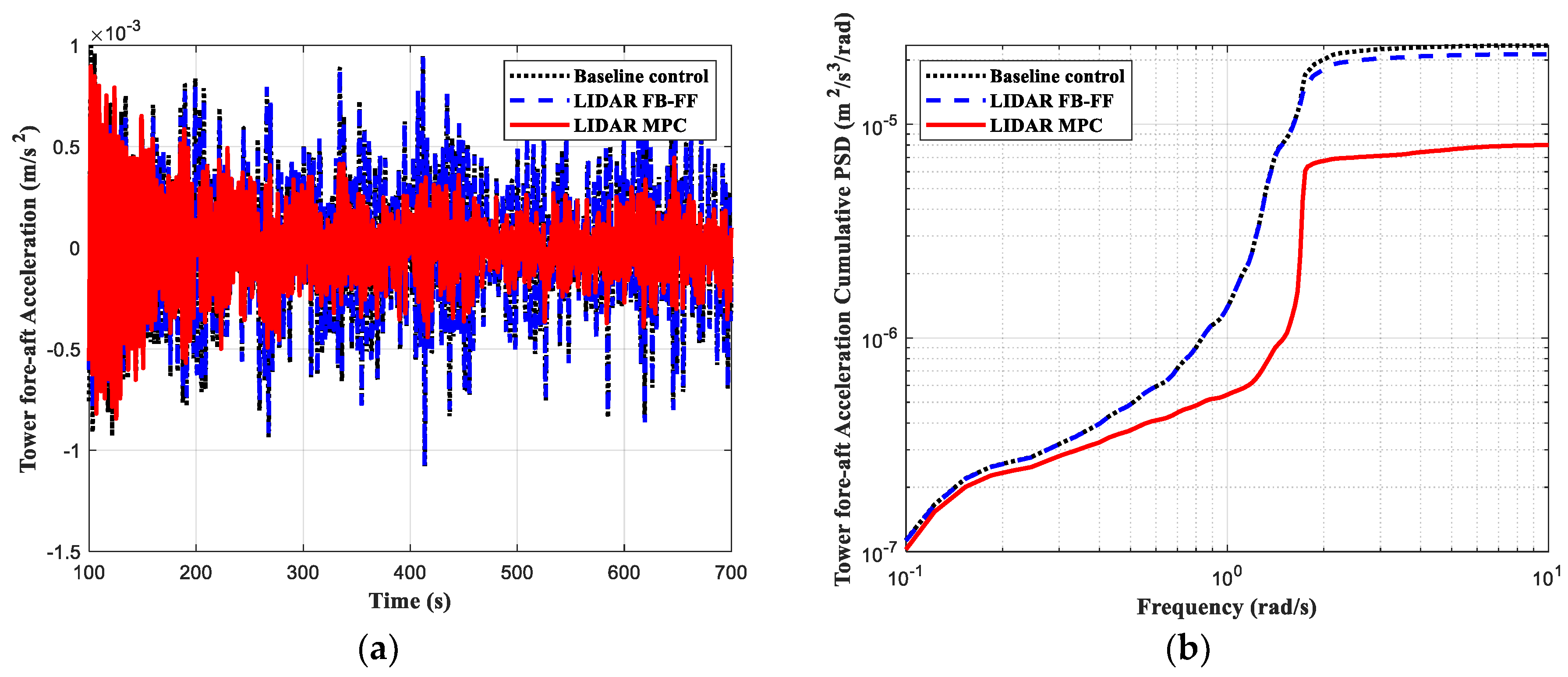
Tower fore-aft acceleration: (a) time profiles; (b) cumulative PSD (for wind speed with 5% turbulence intensity).

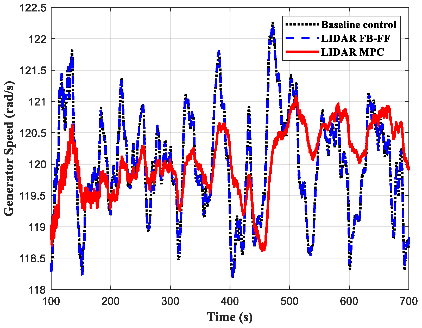
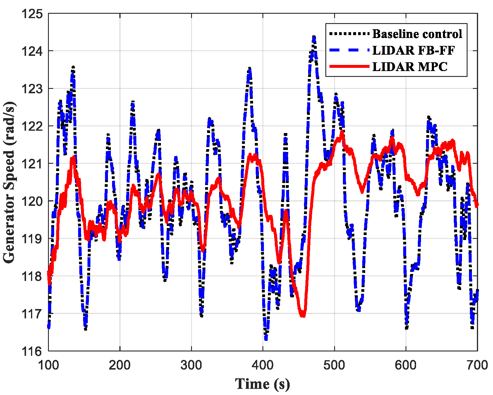
Figure 6.
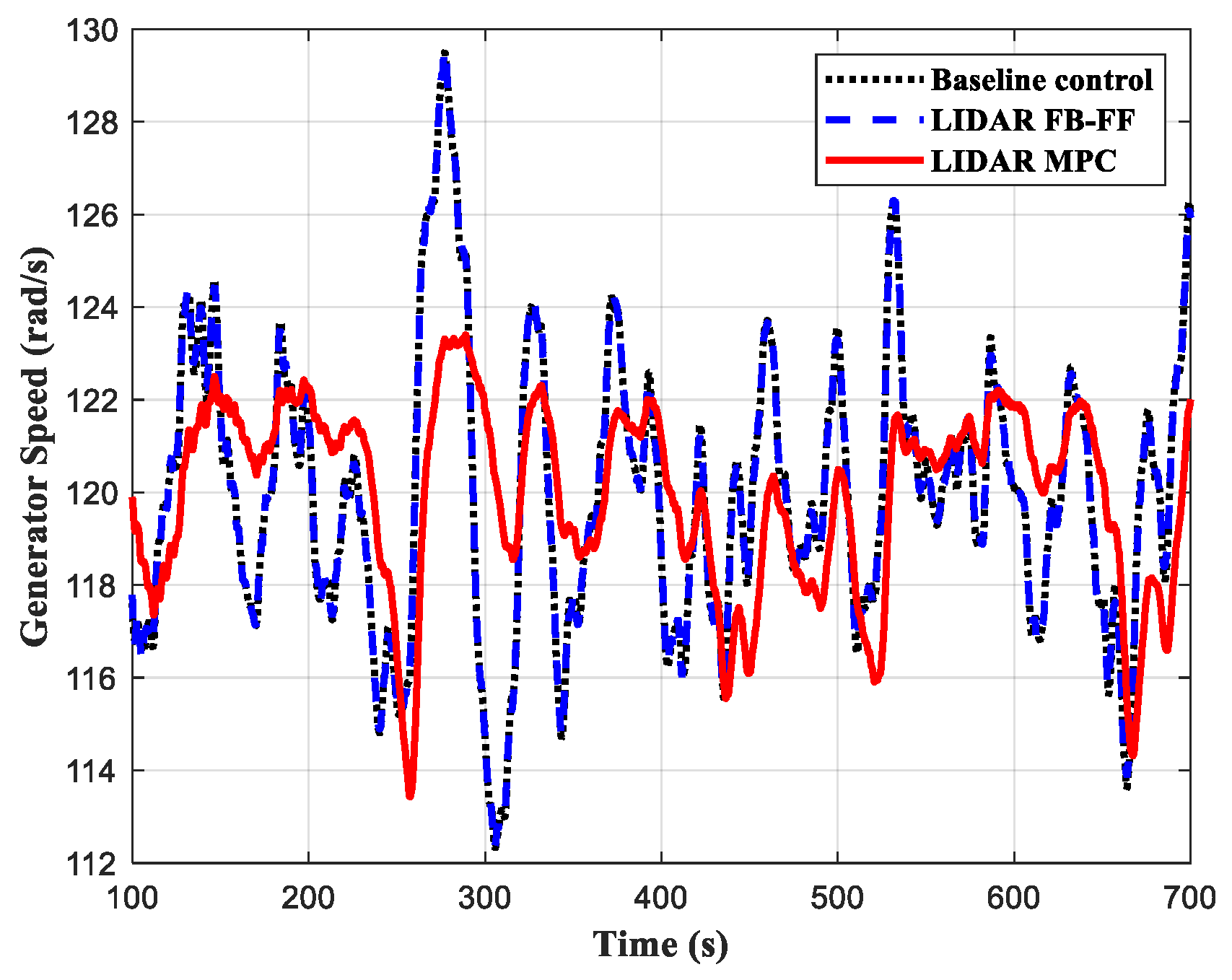
Comparison of generator speeds (wind speed with 5% turbulence intensity).
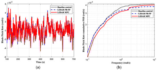
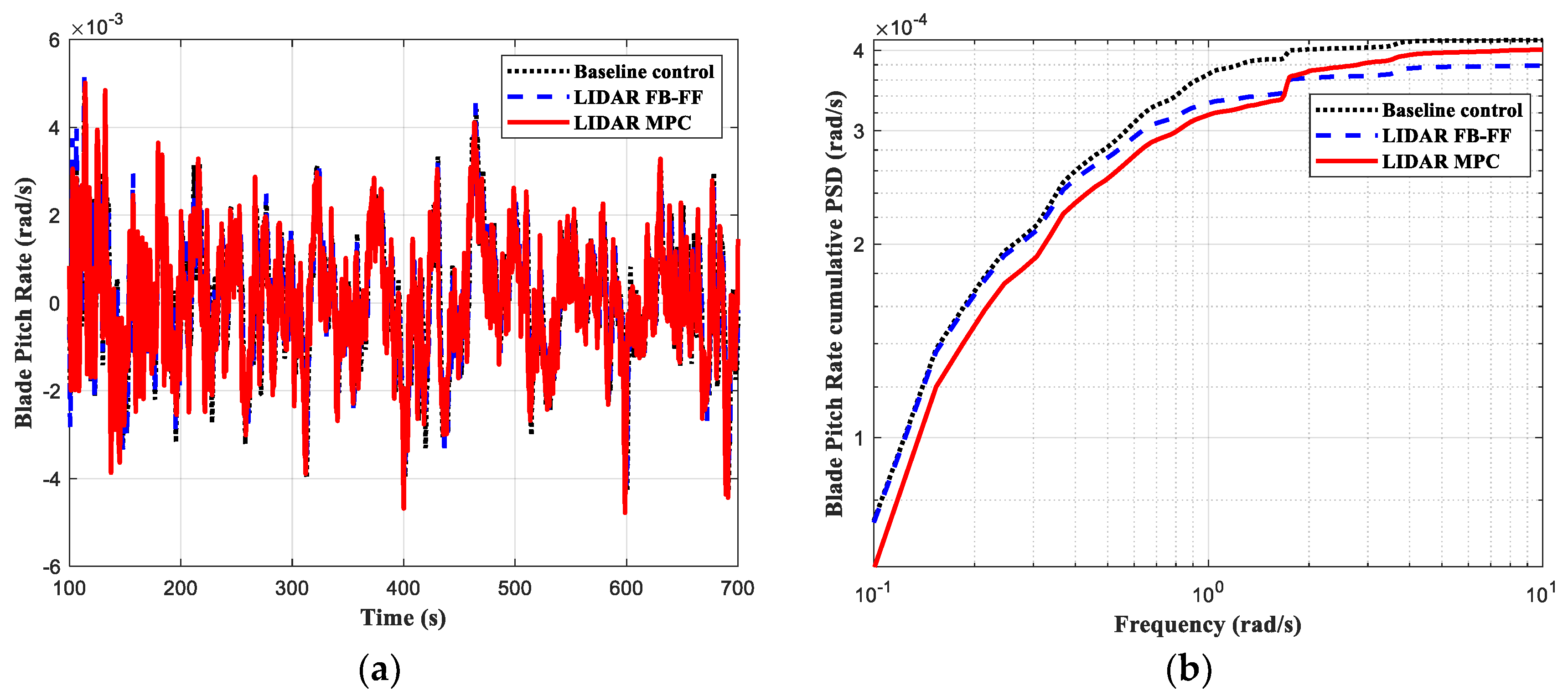
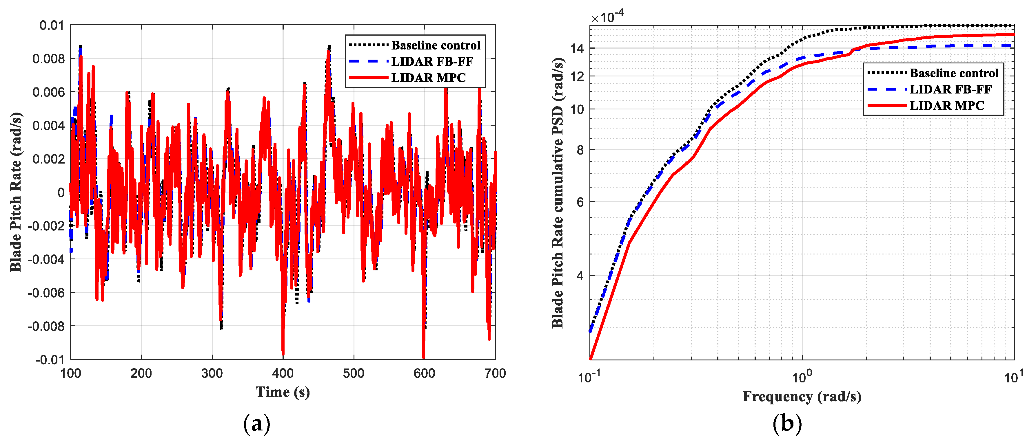
Figure 7.
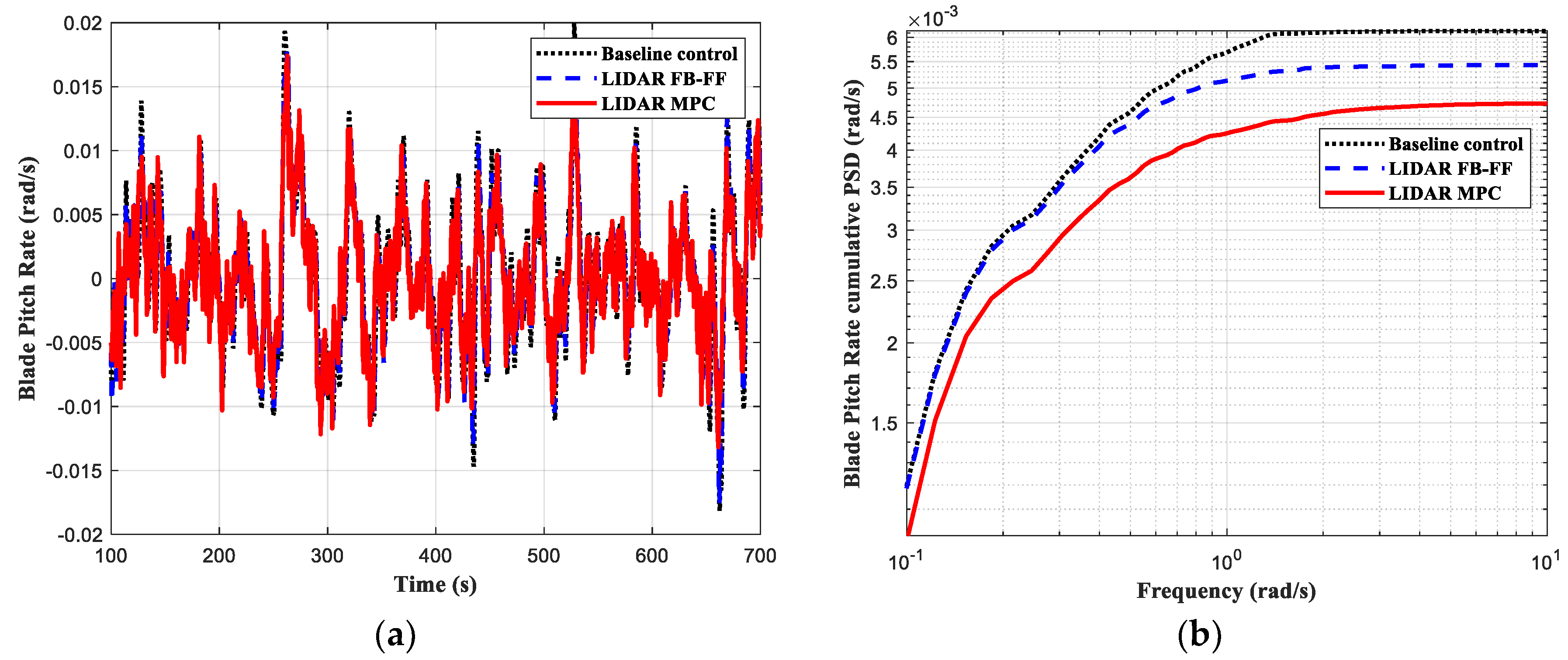
Blade pitch rate: (a) time profiles; (b) cumulative PSD (wind speed with 5% turbulence intensity).
Table 3.
Performance statistics for a wind speed with 5% turbulence intensity.
Figure 4a demonstrates that, compared with the baseline control and the FB-FF control, the MPC design achieved a smaller variation in rotor torque. The statistical time domain results in Table 3 show that the MPC design achieved a 25.68% reduction in rotor torque standard deviation compared to the baseline control.
The cumulative power spectral density (PSD) was calculated to compare the load reduction performance in the frequency domain. As shown in Figure 4b, the FB-FF design achieved a reduction in rotor load compared with the baseline feedback control, but the MPC attained a much better rotor load reduction compared to the other controllers.
Figure 5 presents the results of the tower fore-aft acceleration for each design. In the time domain results, as illustrated in Figure 5a, the MPC showed larger fluctuations in the first few seconds, then the measured values became smaller compared to those obtained from the baseline control and the FB-FF control. This is more clearly seen in Table 3 that shows that the FB-FF control led to a reduction of 11.72% in the tower fore-aft acceleration standard deviation, compared with the baseline control, while the MPC presented a slightly higher standard deviation (−5.03%).
The cumulative PSD for the tower fore-aft acceleration is shown in Figure 5b. The baseline control and the FB-FF control showed similar results, whereas the MPC showed a clearer reduction compared to the other two control algorithms in the working frequency range including the key frequency point of 1 rad/s.
Figure 6 illustrates the simulation results of the wind turbine generator speed. During the above-rated operation, the control objective is to maintain the generator speed at its rated level, which was 120 rad/s in this work. As shown in Figure 6, the FB-FF design had a similar speed regulation performance as the baseline design, while the MPC design achieved a better generator speed tracking performance, which corresponded to a 37.06% reduction in the speed standard deviation, as presented in Table 3.
Finally, the blade pitching rates of the three designs are depicted in Figure 7. It can be observed that the three controllers achieved very close results in the time domain. In the frequency domain, as depicted in Figure 7b, the MPC showed the lowest cumulative PSD in pitch rate over most of the frequency range including the most critical point of 1 rad/s. Both the LIDAR FB-FF control and the LIDAR MPC showed a lower cumulative PSD in pitch rate than the baseline control.
4.3. Wind Speed with 10% Turbulence Intensity
The wind speed in this simulation had a turbulence intensity of 10%, as shown in Figure 3b. Figure 8, Figure 9, Figure 10 and Figure 11 depict the result comparisons of the three controllers, and Table 4 presents the results of standard deviation and the reduction rate of the std for FB-FF and MPC compared to the baseline control.

Figure 8.
Out-of-plane rotor torque: (a) time profiles; (b) cumulative PSD (for wind speed with 10% turbulence intensity).
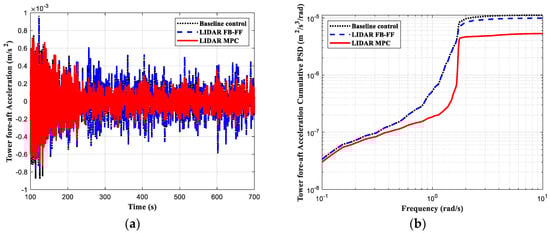
Figure 9.
Tower fore-aft acceleration: (a) time profiles; (b) cumulative PSD (for wind speed with 10% turbulence intensity).

Figure 10.
Comparison of the generator speed (wind speed with 10% turbulence intensity).

Figure 11.
Blade pitch rate: (a) time profiles; (b) cumulative PSD (wind speed with 10% turbulence intensity).
Table 4.
Performance statistics for a wind speed with 10% turbulence intensity.
As demonstrated in Figure 8, the FB-FF control showed a reduction in cumulative PSD of the out-of-plane rotor torque in Figure 8b, compared with the baseline control, while in the time domain, as depicted in Figure 8a, the results of the FB-FF and the baseline control were similar. The MPC design results in both time and frequency domain appeared to be better than those of the other two methods. A reduction of 25.81% of the rotor torque standard deviation was achieved for the MPC compared with the baseline control, as shown in Table 4.
The simulation results of the tower fore-aft acceleration are depicted in Figure 9. The statistics of the three results are compared in Table 4, from which it can be seen that MPC achieved the smallest variation, and the FB-FF is also better than the baseline control. The FB-FF control achieved an 8.9% reduction in the tower fore-aft acceleration standard deviation compared to the baseline control, and the MPC design achieved a reduction of 21.45%. In the frequency domain, as demonstrated in Figure 9b, a lower cumulative PSD could be observed in the FB-FF control compared with the baseline control. The MPC design again achieved the best performance among the three controllers, as shown in both time domain and frequency domain.
Figure 10 illustrates the control result comparison for the generator speed. It can be observed that the results of the baseline and the FB-FF control were similar, while the MPC design led to a better generator speed tracking performance, which was supported by the statistical results in Table 4, where a 41.14% reduction in the standard deviation of the generator speed was achieved by the MPC design.
The pitching rates of the three control designs are depicted in Figure 11. The control results were similar in the time domain, as shown in Figure 11a. Table 4 presents the statistics of the pitching rates time series, which show that the LIDAR FB-FF control result was slightly better than that of the LIDAR MPC, but both showed smaller variations in the pitching rate compared to the results of the baseline control. In the frequency domain, as shown in Figure 11b, both the FB-FF and the MPC design presented a better performance than the baseline control. In the frequency range of interests, the cumulative PSD for the MPC was lower than that for the FB-FF control.
4.4. Wind Speed with 15% Turbulence Intensity
As shown in Figure 3c, the wind speed with a turbulence intensity of 15% varied over a wide range, roughly from 13 to 23 m/s, covering most of the above-rated region. The simulation results of the three controllers are shown in Figure 12, Figure 13, Figure 14 and Figure 15 and in Table 5.
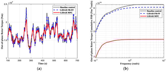
Figure 12.
Out-of-plane rotor torque: (a) time profiles; (b) cumulative PSD (for wind speed with 15% turbulence intensity).
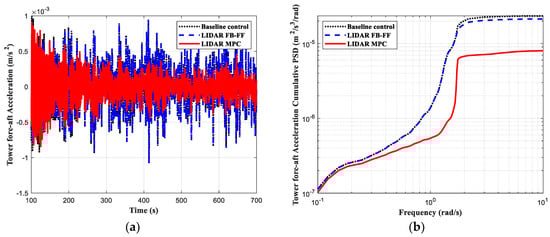
Figure 13.
Tower fore-aft acceleration: (a) time profiles; (b) cumulative PSD (for wind speed with 15% turbulence intensity).
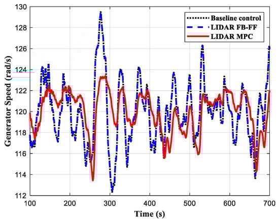
Figure 14.
Comparison of the generator speed (wind speed with 15% turbulence intensity).
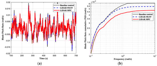
Figure 15.
Blade pitch rate: (a) time profiles; (b) cumulative PSD (wind speed with 15% turbulence intensity).
Table 5.
Performance statistics for a wind speed with 15% turbulence intensity.
The out-of-plane rotor torques are depicted in Figure 12. As shown by both the time domain and the frequency domain results, the FB-FF control and the baseline control showed similar performance, and the LIDAR MPC demonstrated a much lower variation in the rotor torque, which is a significant improvement for load reduction.
It can be seen in Table 5 that, compared with the baseline control, the FB-FF control achieved a small reduction in the out-of-plane rotor torque standard deviation, which was 2.59%. The MPC had a much better performance, obtaining a reduction of 28.67%.
The simulations of the tower fore-aft accelerations are shown in Figure 13. Consistent observations were made as to the rotor torque under the three control strategies. Again, the FB-FF control showed similar results as those of the baseline control, while with the MPC, the variation in the tower fore-aft acceleration was the lowest in comparison with those measured using the other designs.
The same conclusions are reported in Table 5, in which the reduction of the tower fore-aft acceleration standard deviation, compared with that of the baseline control, was 7.07% for the FB-FF control and 32.79% for the MPC design.
Figure 14 illustrates the comparison of the generator speeds. Compared to the FB-FF control and the baseline control, the MPC achieved a largely improved tracking performance, which resulted in a 33.33% reduction of the generator speed standard deviation (see Table 5).
Finally, we compared the blade pitching rates obtained with the three control methods; the results are presented in Figure 15. The MPC achieved a smaller pitching rate variation, as evidenced in both the time domain and the frequency domain results, compared to the other two controls. Table 5 presents the statistical results, showing that the FB-FF control led to a 5.98% reduction in the pitch rate compared with the baseline control, and the MPC achieved a reduction of 13.58% in standard deviation.
4.5. Discussion
In the previous Section 4.2, Section 4.3 and Section 4.4, the control results for the baseline control, the LIDAR-assisted FB-FF control and the designed LIDAR-assisted MPC were presented and compared under three turbulence intensities, i.e., 5%, 10% and 15%, for the same mean wind speed. The statistical results of the three controls under different wind conditions are presented in Table 3, Table 4 and Table 5.
Compared with the baseline control and the LIDAR FB-FF control, under the three wind conditions, the LIDAR MPC design achieved a better performance in most cases with regard to rotor load reduction, generator speed regulation and tower load reduction. The improvement in the generator speed control was clear in all cases. This is probably because the term of generator speed regulation is directly included in the objective function of the MPC.
One exception regarding the MPC is in the tower fore-aft acceleration under 5% turbulence intensity. In this case, the MPC did not achieve a better result than the baseline control. In this wind condition, the LIDAR FB-FF control showed a better control performance on tower load reduction compared to the baseline control.
It can be observed that, with the increase of the wind turbulence intensity, the performance improvement of the LIDAR FB-FF control, compared with the baseline control, was at a constant level, while the MPC performance improvements increased.
Under the three wind conditions, the pitching rate variations had similar time profiles for the three control designs. The MPC results were always better compared to those of the baseline control, though within a small margin, but they were not better than the those of the FB-FF control under 5 and 10% turbulence intensities.
The control of a wind turbine is subject to the external wind disturbance. Our simulations showed that the LIDAR MPC’s performance improvement was more apparent when the wind disturbance level was high. One advantage of the MPC is that it is less dependent on the model accuracy, including model parameters and disturbance. This is due to the receding-horizon optimisation mechanism in the MPC. In the three wind turbine controller designs, linearised turbine models were used, which inevitably introduced a mismatch between the controller design model and the nonlinear system model. It should be noted that the control actions designed based on the linearised model were applied to the nonlinear turbine system. When the turbulence intensity was high, the wind speed varied in a large range, producing a large model uncertainty. This had a greater influence on the performance of the baseline control and the LIDAR FB-FF control than on that of the MPC, since the model output and control input were re-calculated at each sampling time.
The use of a Kalman filter as a state observer is another adaptive factor of the MPC design configuration. The states are updated at each sampling time, which improves the prediction model. Therefore, among the three controllers, the MPC is the best in coping with model uncertainties and disturbances.
Compared to the baseline control and the FB-FF control, the MPC considers more tuning parameters, allowing a larger freedom to tune the controller for the desired performance. The control input is calculated by an optimisation method in the MPC, which is completely different from what occurs with the other two controllers. As a result, the MPC achieves better control performance in most cases.
5. Conclusions
In this paper, a LIDAR-based MPC is proposed for the above-rated wind turbine control. The controller was designed based on a linearised model, and the incoming wind was generated by a LIDAR simulator. The simulations were conducted in a 5 MW nonlinear wind turbine model. A mean wind speed of 18 m/s was selected with turbulence intensities of 5%, 10% and 15%. The MPC design was compared with two other designs, one being the well accepted baseline control, and the other the LIDAR-assisted FB-FF control.
According to the simulation results, all three controllers worked well for the above-rated turbine operation in this study. Among them, the LIDAR FB-FF control produced similar, but slightly better, results as the baseline control. The LIDAR MPC achieved the best performance in most comparisons, especially in the presence of higher wind turbulence intensities.
Both the baseline control and the LIDAR FB-FF control share the same gain-scheduling feedback control. The difference between these two designs is that an added feedforward control channel is present in the FB-FF control scheme, in which the preview wind from the LIDAR simulator is introduced. That is perhaps the main reason why these two controls showed similar results as regards their performance. The MPC is a completely different design, as it calculates the control signals through a constrained optimisation scheme. It is based on the receding horizon optimisation mechanism; therefore, it is less dependent on the model quality. The MPC has also more tuning parameters, which once properly tuned, provide a better chance to achieve the desired performance.
The LIDAR-assisted MPC achieved a good control performance, but it also involves additional costs related to the LIDAR equipment and to a more complex design of the control system. In our current study, the MPC was designed for the above-rated operation control. Further research to extend the MPC to the full envelope of a turbine operation will be conducted in the future.
Author Contributions
Conceptualization, J.B. and H.Y.; Formal analysis, H.Y.; Investigation, J.B.; Methodology, J.B. and H.Y.; Resources, H.Y.; Software, J.B.; Supervision, H.Y.; Validation, J.B. and H.Y.; Writing—original draft, J.B.; Writing—review & editing, J.B. and H.Y. All authors have read and agreed to the published version of the manuscript.
Funding
This research received no external funding.
Informed Consent Statement
Not applicable.
Conflicts of Interest
The authors declare no conflict of interest.
Nomenclature
| θR | Rotor in-plane rotational displacement |
| Rotor in-plane rotational speed | |
| Rotor in-plane rotational acceleration | |
| θT | Tower side-to-side displacement |
| Tower side-to-side speed | |
| Tower side-to-side acceleration | |
| θH | Hub rotational displacement |
| Hub rotational speed | |
| θG | Generator rotational displacement |
| Generator rotational speed | |
| Generator rotational acceleration | |
| ΦR | Rotor out-of-plane displacement |
| Rotor out-of-plane speed | |
| Rotor out-of-plane acceleration | |
| ΦT | Tower fore-aft displacement |
| Tower fore-aft speed | |
| Tower fore-aft acceleration | |
| Qin | In-plane aerodynamic torque on the rotor |
| Qout | Out-of-plane aerodynamic torque on the rotor |
| J | Rotor inertia |
| Jt | Tower fore-aft inertia |
| Jc | Rotor/tower cross coupling inertia |
| Jts | Tower side-to-side inertia |
| IHs | Sum of generator and high-speed shaft inertia |
| Ke | Blade edge-wise stiffness |
| Kf | Blade flap-wise stiffness |
| Kt | Tower fore-aft stiffness |
| Kts | Tower side-to-side stiffness |
| Bt | Tower fore-aft damping moment |
| Bts | Tower side-to-side damping moment |
| TLs | Gearbox torque at low-speed shaft |
| THs | Gearbox torque at high-speed shaft |
| TG | Generator torque |
| gHs | High-speed shaft damping |
| N | Gearbox ratio |
| β | Blade pitch angle |
Abbreviations
| LIDAR | Light Detection and Ranging |
| FB-FF | Combined Feedback and Feedforward |
| MPC | Model Predictive Control |
| PI(D) | Proportional–Integral(–Derivative) |
| IPC | Individual Pitch Control |
| IBC | Individual Blade Control |
| PSD | Power Spectral Density |
References
- Council, G.W.E. GWEC| Global Wind Report 2022; Global Wind Energy Council: Brussels, Belgium, 2022. [Google Scholar]
- Leithead, W.; Connor, B. Control of variable speed wind turbines: Dynamic models. Int. J. Control 2000, 73, 1173–1188. [Google Scholar] [CrossRef]
- Leithead, W.; Connor, B. Control of variable speed wind turbines: Design task. Int. J. Control 2000, 73, 1189–1212. [Google Scholar] [CrossRef]
- Chatzopoulos, A.-P. Full Envelope Wind Turbine Controller Design for Power Regulation and Tower Load Reduction. Ph.D. Thesis, University of Strathclyde, Glasgow, UK, 2011. [Google Scholar]
- Bossanyi, E. The design of closed loop controllers for wind turbines. Wind Energy 2000, 3, 149–163. [Google Scholar] [CrossRef]
- Bossanyi, E. Wind turbine control for load reduction. Wind Energy 2003, 6, 229–244. [Google Scholar] [CrossRef]
- Leithead, W.; Dominguez, S.; Spruce, C. Analysis of Tower/Blade Interaction in the Cancellation of the Tower Fore-Aft Mode via Control. In Proceedings of the European Wind Energy Conference 2004, London, UK, 22–25 November 2004; EWEA: London, UK, 2004. [Google Scholar]
- Leithead, W.; Dominguez, S. Controller Design for the Cancellation of the Tower Fore-Aft Mode in a Wind Turbine. In Proceedings of the 44th IEEE Conference on Decision and Control, Seville, Spain, 12-15 December 2005; IEEE: Seville, Spain, 2005; pp. 1276–1281. [Google Scholar]
- Bossanyi, E. Individual blade pitch control for load reduction. Wind Energy 2003, 6, 119–128. [Google Scholar] [CrossRef]
- Bossanyi, E. Further load reductions with individual pitch control. Wind Energy 2005, 8, 481–485. [Google Scholar] [CrossRef]
- Han, Y.; Leithead, W. Combined Wind Turbine Fatigue and Ultimate Load Reduction by Individual Blade Control. J. Phys. Conf. Ser. 2014, 524, 012062. [Google Scholar] [CrossRef]
- Schlipf, D.; Kühn, M. Prospects of a collective pitch control by means of predictive disturbance compensation assisted by wind speed measurements. In Proceedings of the 9th German Wind Energy Conference DEWEK, Bremen, Germany, 26–27 November 2008; EWEA: Bremen, Germany, 2008. [Google Scholar]
- Dunne, F.; Pao, L.Y.; Wright, A.D.; Jonkman, B.; Kelley, N. Combining Standard Feedback Controllers with Feedforward Blade Pitch Control for Load Mitigation in Wind Turbines. In Proceedings of the 48th AIAA Aerospace Sciences Meeting (AIAA 2010), Orlando, FL, USA, 4–7 January 2010. [Google Scholar]
- Dunne, F.; Pao, L.Y.; Wright, A.D.; Jonkman, B.; Kelley, N. Adding feedforward blade pitch control to standard feedback controllers for load mitigation in wind turbines. Mechatronics 2011, 21, 682–690. [Google Scholar] [CrossRef]
- Laks, J.; Pao, L.; Wright, A.; Kelley, N.; Jonkman, B. The use of preview wind measurements for blade pitch control. Mechatronics 2011, 21, 668–681. [Google Scholar] [CrossRef]
- Wang, N.; Johnson, K.E.; Wright, A.D. FX-RLS-based feedforward control for LIDAR-enabled wind turbine load mitigation. IEEE Trans. Control Syst. Technol. 2012, 20, 1212–1222. [Google Scholar] [CrossRef]
- Schlipf, D. Prospects of multivariable feedforward control of wind turbines using lidar. In Proceedings of the American Control Conference (ACC), Boston, MA, USA, 6–8 July 2016; pp. 1393–1398. [Google Scholar]
- Mikkelsen, T.; Angelou, N.; Hansen, K.; Sjöholm, M.; Harris, M.; Slinger, C.; Hadley, P.; Scullion, R.; Ellis, G.; Vives, G. A spinner-integrated wind lidar for enhanced wind turbine control. Wind Energy 2013, 16, 625–643. [Google Scholar] [CrossRef]
- Fleming, P.A.; Scholbrock, A.; Jehu, A.; Davoust, S.; Osler, E.; Wright, A.D.; Clifton, A. Field-Test Results Using a Nacelle-mounted Lidar for Improving Wind Turbine Power Capture by Reducing Yaw Misalignment. J. Phys. Conf. Ser. 2014, 524, 012002. [Google Scholar] [CrossRef]
- Kragh, K.A.; Hansen, M.H. Load alleviation of wind turbines by yaw misalignment. Wind Energy 2014, 17, 971–982. [Google Scholar] [CrossRef]
- Soliman, M.; Malik, O.; Westwick, D. Multiple model MIMO predictive control for variable speed variable pitch wind turbines. In Proceedings of the 2010 American Control Conference, Baltimore, MD, USA, 30 June–2 July 2010; pp. 2778–2784. [Google Scholar]
- Gros, S.; Schild, A. Real-time economic nonlinear model predictive control for wind turbine control. Int. J. Control 2017, 90, 2799–2812. [Google Scholar] [CrossRef]
- Kong, X.; Ma, L.; Liu, X.; Abdelbaky, M.A.; Wu, Q. Wind turbine control using nonlinear economic model predictive control over all operating regions. Energies 2020, 13, 184. [Google Scholar] [CrossRef]
- Hussain, R.; Yue, H.; Recalde-Camacho, L. Model Predictive Control of Wind Turbine with Aero-Elastically Tailored Blades. J. Phys. Conf. Ser. 2022, 2265, 032084. [Google Scholar] [CrossRef]
- Laks, J.; Pao, L.Y.; Simley, E.; Wright, A.; Kelley, N.; Jonkman, B. Model predictive control using preview measurements from lidar. In Proceedings of the 49th AIAA Aerospace Sciences Meeting, Orlando, FL, USA, 4–7 January 2011. [Google Scholar]
- Bottasso, C.; Pizzinelli, P.; Riboldi, C.; Tasca, L. LiDAR-enabled model predictive control of wind turbines with real-time capabilities. Renew. Energy 2014, 71, 442–452. [Google Scholar] [CrossRef]
- Schlipf, D.; Schlipf, D.J.; Kühn, M. Nonlinear model predictive control of wind turbines using LIDAR. Wind Energy 2013, 16, 1107–1129. [Google Scholar] [CrossRef]
- Bossanyi, E. GH Bladed-User Manual, Version 4.4; Garrad Hassan: Bristol, UK, 2013. [Google Scholar]
- Bao, J.; Yue, H.; Leithead, W.E.; Wang, J.-Q. Feedforward control for wind turbine load reduction with pseudo-LIDAR measurement. Int. J. Autom. Comput. 2018, 15, 142–155. [Google Scholar] [CrossRef] [Green Version]
- Leithead, W.E.; Rogers, M.C.M. Drive-train characteristics of constant speed HAWT’s: Part I-representation by simple dynamic models. Wind Eng. 1996, 20, 149–174. [Google Scholar]
- Leithead, W.E.; Rogers, M.C.M. Drive-train characteristics of constant speed HAWT’s: Part II-simple characterisation of dynamics. Wind Eng. 1996, 20, 175–201. [Google Scholar]
- MathWorks. MATLAB Primer, R2020b ed.; MathWorks: Natick, MA, USA, 2020. [Google Scholar]


Publisher’s Note: MDPI stays neutral with regard to jurisdictional claims in published maps and institutional affiliations. |
© 2022 by the authors. Licensee MDPI, Basel, Switzerland. This article is an open access article distributed under the terms and conditions of the Creative Commons Attribution (CC BY) license (https://creativecommons.org/licenses/by/4.0/).