Mapping Methodology for Self and Mutual Inductance Profiles in IPT Systems

Abstract

Magnetic couplers (MC) are the key element that enable the power transfer over large air gaps in inductive power transfer (IPT) systems. Numerous designs with different coil and core arrangements have been proposed in the literature. However, the MC sizing process still involves several trial and error iterations to meet the desired specifications. This paper presents a profile methodology that uses fitting equations to extrapolate the coupling profiles and minimize the required number of finite element analysis (FEA) simulation results. A non-polarized circular coupler (FLCP) can be characterized as function of the air gap and lateral displacements using only six charging positions, whereas polarized couplers, such as the bipolar (BPP) or double-D pad (DDP), can be characterized using 18 charging positions. The methodology is validated experimentally using the FLCP, and an average error of 3% was found under different charging positions.

1. Introduction

Inductive power transfer (IPT) technology is an efficient alternative to plug-in electric vehicle (EV) chargers. The absence of contacts between the off-board and the vehicle’s side offers new charging possibilities with the vehicle in movement, operation under different weather conditions, and even in submerged scenarios, without the risk of electrocution.

IPT systems accomplish power transfer by means of a loosely coupled transformer, also known as magnetic coupler (MC). Each side of the MC, referred in this work as transmitter and receiver pads, is formed by one or more coils, a ferromagnetic core, and shield (optional). The spatial freedom of the receiver pad towards the transmitter pad, both vertical and lateral displacements, reduce the coupling of the MC. Numerous geometries have been presented in the literature with optimized core arrangements and new coil configurations to boost the coupling factor [1,2,3,4]. Intermediate couplers were also introduced between the transmitter and receiver pads to further increase the vertical tolerance [5,6,7,8,9].

The spatial freedom of the receiver pad, placed under the vehicle, and the driver’s tolerance to park the vehicle over the transmitter pad creates a charging area where the EV IPT charger must operate. As a consequence, the coupling profile will differ according to vertical and lateral displacements. Furthermore, the power-transfer capabilities of the IPT system are affected at lower coupling scenarios, and optical positioning systems are usually employed to maximize the coupling value. Additionally, wireless communication between the off-board and the vehicle’s side is often required to exchange information regarding batteries status and vehicle positioning. New mutual inductance and load estimation algorithms have been presented in the literature using only measurements from the off-board side [10,11,12,13]. Such algorithms, when coped with the mutual inductance profile, can be used as a guiding positioning system, thus eliminating the use of optical sensors.

Self and mutual inductance profiling as a function of different vertical and lateral displacements is usually performed using mathematical models or Finite Element Analysis (FEA) tools. However, the mathematical models [14,15], are usually valid for a specific coil geometry and core arrangement, which limits the study of new MC geometries. FEA tools, on the other hand, offer unconstrained design capabilities. The authors in [16] present a framework that evaluates different transmitter and receiver pad sizes in different charging positions and at different output powers using the DD pad. The framework combines the mathematical model of an IPT system with the self and mutual inductance profiles of the MC obtained through a Finite Element Analysis (FEA) tool. A total of 11648 FEA simulations were required to extract the profiles of the MC with a fixed number of turns in each coil. However, the computational effort and time consumption drastically increases if different turn arrangements are considered.

This paper presents a mapping methodology for self and mutual inductance profiles for static IPT systems with a reduced computational effort. A behavioral analysis of the self and mutual inductance profiles under different turns combinations and vertical and lateral displacements is performed to identify adequate fitting curves. This allows the extraction of minimum number of required charging positions and, consequently, has a positive impact on the required number of FEA simulations. In this way, it is possible to characterize an MC geometry with a specific size and ratio and evaluate its applicability in different IPT systems with different power requirements and operational specifications. Both the fitting curves and the proposed mapping methodology are validated using an FEA tool and, afterwards, are experimentally verified.

The paper starts with a brief description of MC in IPT systems. Section 2 derives the fundamental equations of two- and three-coil IPT systems, and it describes the main MC components and geometries. The fitting approach method is introduced in Section 3. A case study is analyzed in Section 4, and the main conclusions are drawn in Section 5.

2. Magnetic Coupler

2.1. Fundamentals

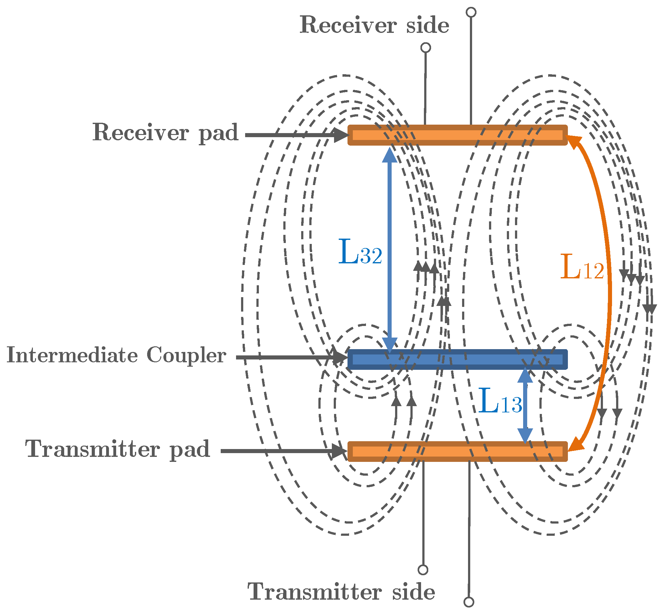
The Magnetic Coupler (MC) is a loosely coupled transformer with a transmitter and receiver pads. Each pad is formed by one or more coils, a ferromagnetic core and a shield (if necessary). Figure 1 illustrates the MC of a two-coil IPT system (represented by the color brown) and the flux lines that link the transmitter and receiver pads. The coupling coefficient ($k_{12}$) between both sides is given by:

$$k_{12}=L_{12}/\sqrt{(L_1·L_2)},$$

(1)

where $L_1$ and $L_2$ are the self-inductance values of the transmitter and receiver coils and $L_{12}$ is the mutual inductance. The subscript numbers in the variables indicate to which side the variable is related to, where 1 and 2 stands for transmitter and receiver sides, respectively. All symbols and acronyms are listed in the Abbreviationsof the manuscript.

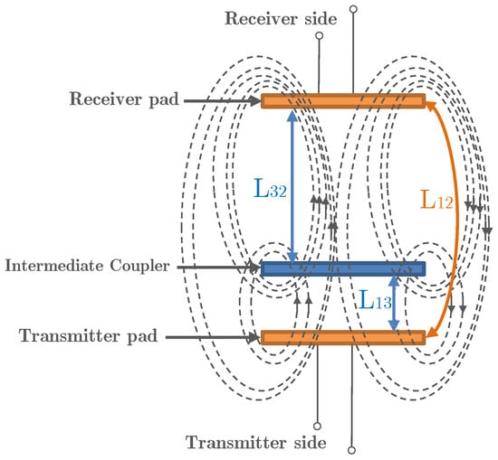
Figure 1. Magnetic coupler with the inclusion of an intermediate coupler.

The self and mutual inductance values of a MC can be determined by the open-circuit test, similar to a conventional 50 Hz transformer. The open-circuit test consists on supplying a pad with the nominal voltage (${\overline{V}}_x$) while the other pad remains open. The open-circuit voltage (${\overline{V}}_{oc}$), no-load power ($P_{oc}$) and no-load current (${\overline{I}}_{oc}$) are then extracted and the self and mutual inductance values are obtained using:

$$L_{xy}=\frac{{\overline{V}}_{o{c}_y}}{j·\omega ·{\overline{I}}_{o{c}_x}},x,y=1,2,3$$

(2)

$$L_x=\frac{Q_{o{c}_x}}{{\omega }^2·{\left|{\overline{I}}_{o{c}_x}\right|}^2},x=1,2,3$$

(3)

where $Q_{o{c}_x}$ is the no-load reactive power, and it is determined by:

$$Q_{o{c}_x}=\sqrt{\left(\right|{\overline{V}}_x|·|{\overline{I}}_{o{c}_x}{\left|\right)}^2-P_{o{c}_x}^2},x=1,2,3$$

(4)

The open-circuit test is performed to each coil in order to fully characterize an MC.

The inclusion of an intermediate coupler (IC) in two-coil IPT systems boosts the magnetic link between the transmitter and receiver, and this new IPT configuration is commonly referred to as a three-coil system. The IC is formed by an intermediate coil ($L_3$) connected in series with a capacitor ($C_3$), and it is usually tuned with a frequency higher than the operating frequency. The subscript number 3 identifies the variables from the intermediate side. Figure 1 illustrates the inclusion of an IC (represented in blue) between the transmitter and receiver pads. The intermediate coil creates two additional couplings between the existing transmitter and receiver coils: $k_{32}$ and $k_{13}$. The first quantifies the magnetic link between the receiver and intermediate coils while the second quantifies the magnetic link between the transmitter and intermediate coils. The correspondent mutual inductance values, depicted in Figure 1, are given by:

$$\begin{array}{cc}\hfill L_{32}& =k_{32}·\sqrt{(L_2·L_3)},\hfill \end{array}$$

(5)

$$\begin{array}{cc}\hfill L_{13}& =k_{13}·\sqrt{(L_1·L_3)},\hfill \end{array}$$

(6)

Analogously to two-coil systems, the self and mutual inductance values in three-coil systems are also determined using (2) and (3).

2.2. Geometry

The geometry and total number of coils in an MC pad affect the coupling pattern and the MC tolerance to air gaps and lateral displacements. Single-coil designs, such as the circular pad (CP) [1], are easier to build and use less material at the expense of a limited coupling area between the transmitter and receiver pads. New designs arose in the literature with the introduction of geometries with multiple coils in each pad. Among the most studied in literature are the Double-D pad (DDP), the solenoid pad (SP) [17], the asymmetric quadrature coils and the Bipolar pad (BPP), illustrated in Figure 2a. The main distinctive characteristic of these geometries is the increase in the flux path to approximately half of the pad size. As a consequence, the air gap and lateral gap tolerance along one axis is drastically increased when compared with single-coil designs.

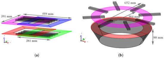
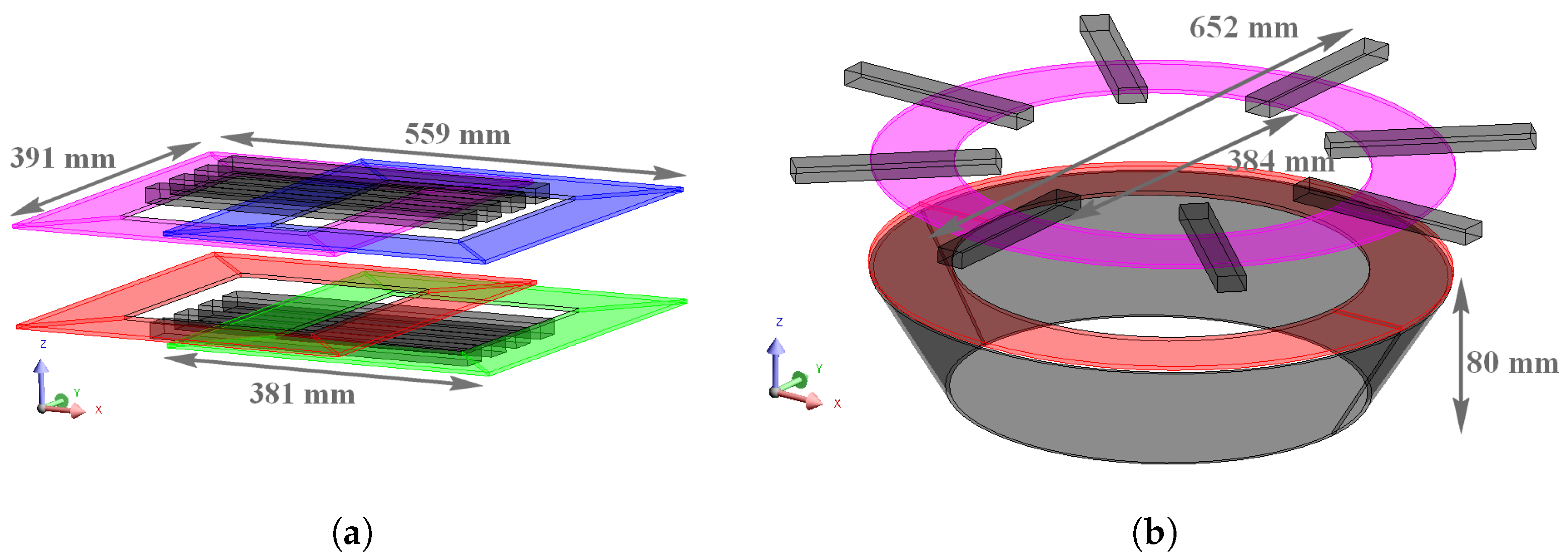
Figure 2. Magnetic coupler geometries: (a) Bipolar pad (BPP), (b) Ferrite-less circular pad (FLCP).

Variants of the aforementioned geometries have been proposed in the literature for dynamic charging applications such as roadways [9,18,19]. The ferromagnetic core is replaced by one or more coils that channels the flux lines between the main power coils. The concrete ferrite-less pad (CFLP) replaced the ferrite core of a DDP with a pipe coil connected in series with the DD coils [18]. Recent studies also show the benefits of inserting intermediate resonators between the transmitter and receiver pads as an alternative to ferromagnetic cores [6,7,9]. The works [6,7] evaluate different circular and rectangular coil geometries in a coplanar fashion. The authors in [9] proposed a ferrite-less circular pad (FLCP), shown in Figure 2b. The use of a shaped cone coil boosts the coupling between the transmitter and receiver sides when used as an IC. The self and mutual inductance profiles of non-polarized and polarized MCs will be subject of study in this work.

3. Characterization of MC

This section explains a curve-fitting-based method that minimizes the number of FEA simulations required to create the self and mutual inductance profiles as a function of air gap ($airgap$), lateral displacement ($l_t$) and $N_x$.

3.1. Mutual Inductance Profiling

The mutual inductance quantifies the flux link between two magnetically coupled coils. This link is affected by the relative position of the coils but also by the number of turns in each coil. Two-coil IPT systems only have one mutual inductance ($L_{12}$) between the transmitter and receiver coils. On the other hand, three-coil systems have two additional mutual inductance values in addition to $L_{12}$, $L_{32}$ and $L_{13}$. In three-coil IPT systems, the intermediate coil is placed in the same enclosure as the transmitter coil [6,7,9], and for that reason, the pattern of $L_{13}$ is almost unaffected by air gap and lateral displacements of the receiver coil, especially in ferrite-less designs. On the other hand, the profile of $L_{13}$ as a function of the number of turns is identical to the profiles of $L_{12}$ and $L_{32}$ in the same conditions, and it will be explained later in this section.

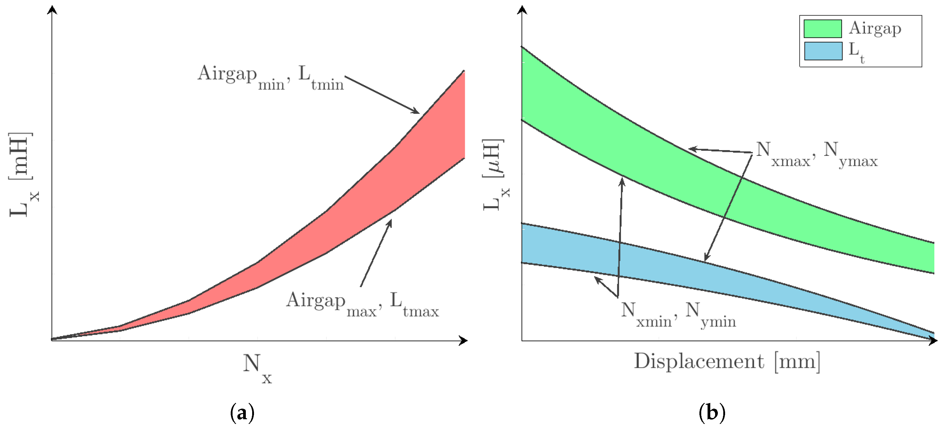
The profiles of $L_{12}$ and $L_{32}$ for different air gaps, lateral displacements and sets of turns values are identical in both three-coil and two-coil systems, and they are illustrated in Figure 3. The colored areas show the effect of having different sets of turns in the coils. The upper and lower boundary lines of the green and blue areas are determined for the pair of turns ($N_{x_{max}}$, $N_{y_{max}}$) and ($N_{x_{min}}$, $N_{y_{min}}$), where x and y denotes the side of the respective coil: transmitter (1), receiver (2) and intermediate (3). The red area illustrates the effect between $N_{y_{min}}$ and $N_{y_{max}}$ for different $N_x$. The values of $N_{x_{min}}$ and $N_{y_{min}}$ are set to 1 while $N_{x_{max}}$ and $N_{y_{max}}$ are limited by the availability of space in the MC or by electric restrictions such as the maximum induced voltage at the coils’ terminals. The plots depicted in Figure 3 were obtained through several FEA simulation results, and they are in compliance with the existing literature for both polarized and non-polarized pads [1,3,9,19,20]. Figure 3a shows the effect of air gap variations in $L_{12}$ and $L_{32}$, and for a given set of turns, it follows an exponential decay function given by:

$$L_{xy}\left(airgap\right)=a_1·e^{b_1·airgap},xy=12orxy=32$$

(7)

where $a_1$ and $b_1$ are constants that depend of $N_x$, $N_y$ and $l_t$.

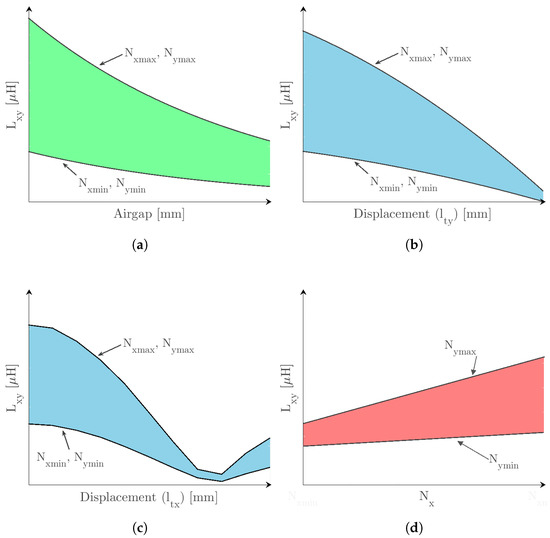
Figure 3. Profiles of $L_{12}$ and $L_{32}$ as a function of (a) $airgap$, (b) $l_{tx}$, (c) $l_{ty}$ and (d) $N_x$.

Similarly, the impact of $l_t$ variations is identical across $L_{12}$ in two-coil systems and $L_{12}$ and $L_{32}$ in three-coil systems. The profile of $l_t$, unlike the $airgap$ pattern, may differ along the x and y axes due to the shape of the MC and to its flux line orientations (polarized or non-polarized MCs). Thus, Figure 3b illustrates the behavior of $L_{12}$ for different lateral displacements along the y axis ($l_{ty}$) with different sets of turns for a circular-shaped MC such as the FLCP and a polarized pad such as the BPP. The behavior of $L_{12}$ as a function of lateral displacements along the x axis ($l_{tx}$) with different sets of turns is depicted in Figure 3c for the BPP. Circular MC designs have the same behavior along the x and y axes, and they only need to be characterized along one axis. The polarized pads have in turn distinct behaviors along both axes due to the total decoupling of one coil along the x axis, which corresponds to the inflection point of $L_{12}$, shown in Figure 3c. Nevertheless, and up to the inflection point, all patterns of $L_{12}$ or $L_{32}$ can be approximated using a Gaussian function defined as:

$$L_{xy}\left(l_t\right)=a_2·e^{-{((l_t-b_2)/c_2)}^2},xy=12orxy=32,$$

(8)

where $a_2$, $b_2$ and $c_2$ are constants that depend on $N_x$ and $l_t$.

The set of turns in two mutually coupled coils also affects the value of the mutual inductance, as illustrated by the colored areas in Figure 3a–c. At a given $airgap$ and $t_t$ charging position, the value of the mutual inductance exhibits a linear variation, described in (9), if one coil is set with a fixed number of turns (value set between $N_{ymin}$ and $N_{ymax}$), while the other coil is winded between $N_{x_{min}}$ and $N_{x_{max}}$, as depicted in Figure 3d:

$$L_{xy\to N_y}\left(N_x\right)=a_3·N_x+b_3,$$

(9)

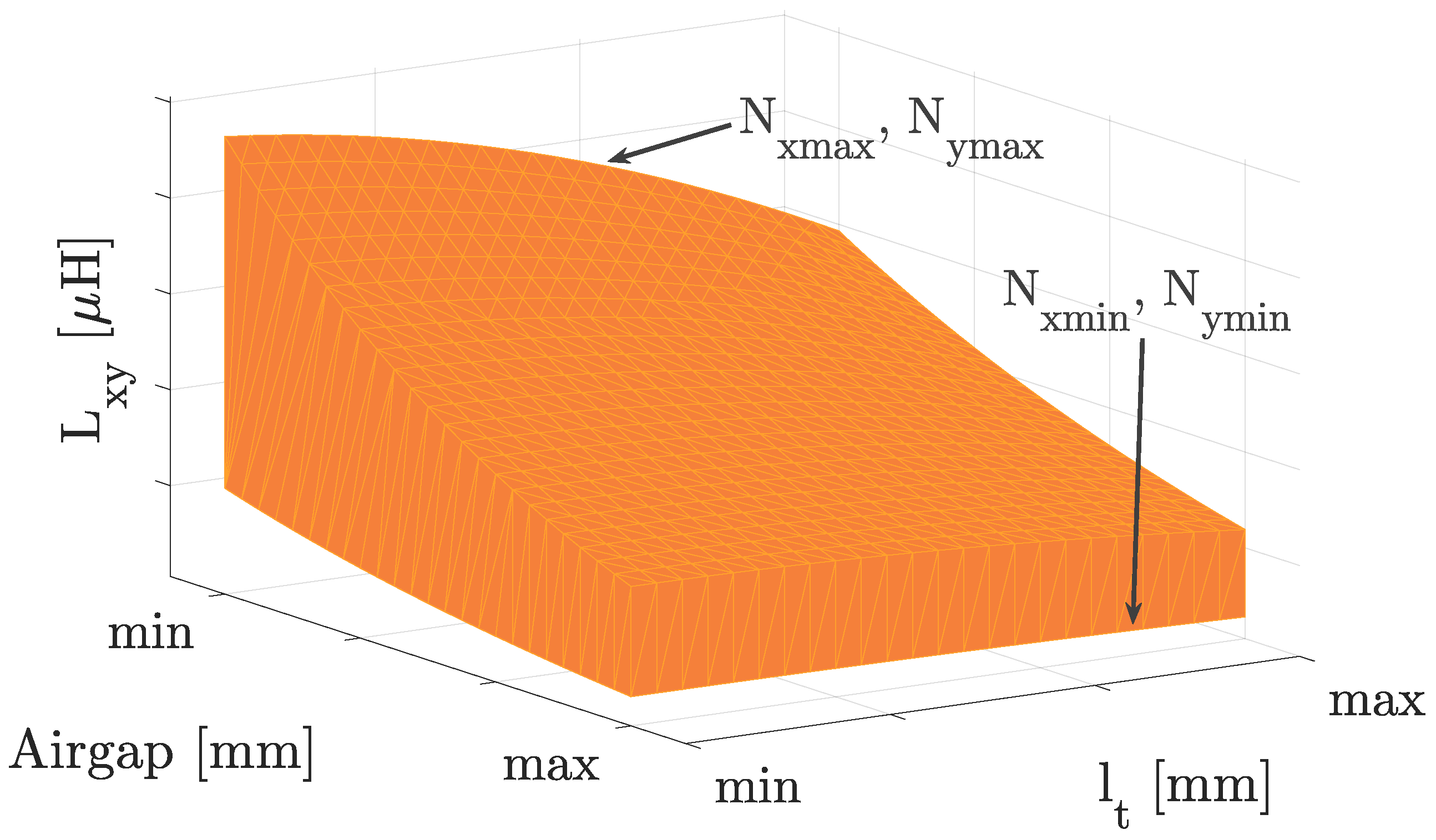
where $a_3$ and $b_3$ correspond to the slope and intersect, respectively. Figure 4 shows the volume of $L_{12}$ and $L_{23}$ as a function of $airgap$, $l_t$, $N_x$ and $N_y$ for the FLCP. The proposed approach takes advantage of the identified patterns represented in Figure 3 to minimize the number of required FEA simulations and creates the volume in Figure 4.

Figure 4. Volume of $L_{xy}$ = f($N_x,N_y,airgap,l_t$).

3.1.1. Methodology

The proposed methodology builds the profile $L_{xy}=f(N_x,N_y,airgap,l_t)$ via an iterative way by varying one or two variables, such as $L_{xy}=f\left(airgap\right)$ or $L_{xy}=f(N_x,N_y)$, while the remaining variables are kept constant. The unknown parameters of functions (7)–(9) that model the effect of $airgap$, $l_t$ and $N_x$ can be found using FEA simulation results. The total number of FEA simulation results required by the proposed approach will vary with the number and type of unknown variables. For example, a full characterization of a circular-shaped MC has four unknown variables ($N_x,N_y,airgap,l_t$) while the remaining MCs have five unknown variables since $l_t$ splits into $l_{tx}$ and $l_{ty}$. In addition, the FEA simulation conditions differ according to the unknown variable. This work introduces the terms $Scenario$ and $Pos$ to differentiate positioning parameters such as $airgap$ and $l_t$ from construction parameters such as the set of turns in FEA simulations.

The term $Pos$, short for position, corresponds to a specific charging location with a given $airgap$ and $l_t$ values. In each $Pos$, if the set of turns is unknown, the proposed approach needs to simulate additional $Scenarios$. Therefore, a $Scenario$ accounts for an FEA simulation in the same $Pos$ but with a different number of turns in each coil.

The effect of the number of turns in one coil can be modeled using (9), as depicted in Figure 3d. The characterization of $L_{xy}=f(N_x,N_y)$, in a given $Pos$, can then be made with resource to, at least, four $Scenarios$ results given by:

$$\begin{array}{cc}\hfill ScenarioA& \to N_x=N_{x_{min}},N_y=N_{y_{min}}\hfill \\ \hfill ScenarioB& \to N_x=N_{x_{max}},N_y=N_{y_{max}}\hfill \\ \hfill ScenarioC& \to N_x=N_{x_{min}},N_y=N_{y_{max}}\hfill \\ \hfill ScenarioD& \to N_x=N_{x_{max}},N_y=N_{y_{min}}.\hfill \end{array}$$

(10)

These scenarios correspond to the four combinations between the maximum and minimum turn numbers. An identical approach is carried out for $L_{xy}=f\left(airgap\right)$ and $L_{xy}=f\left(l_t\right)$ (both $l_{tx}$ and $l_{ty}$), depicted from Figure 3a–c. The first profile is extrapolated from an exponential decay function, whereas the second and third profiles are found using a Gaussian function. The minimum number of points required to find the constant parameters in (7) and (8) are two and three, respectively. In other words, a minimum of two $Pos$ results are needed to characterize $L_{xy}=f\left(airgap\right)$ and a minimum of three $Pos$ results to identify $L_{xy}=f\left(l_t\right)$.

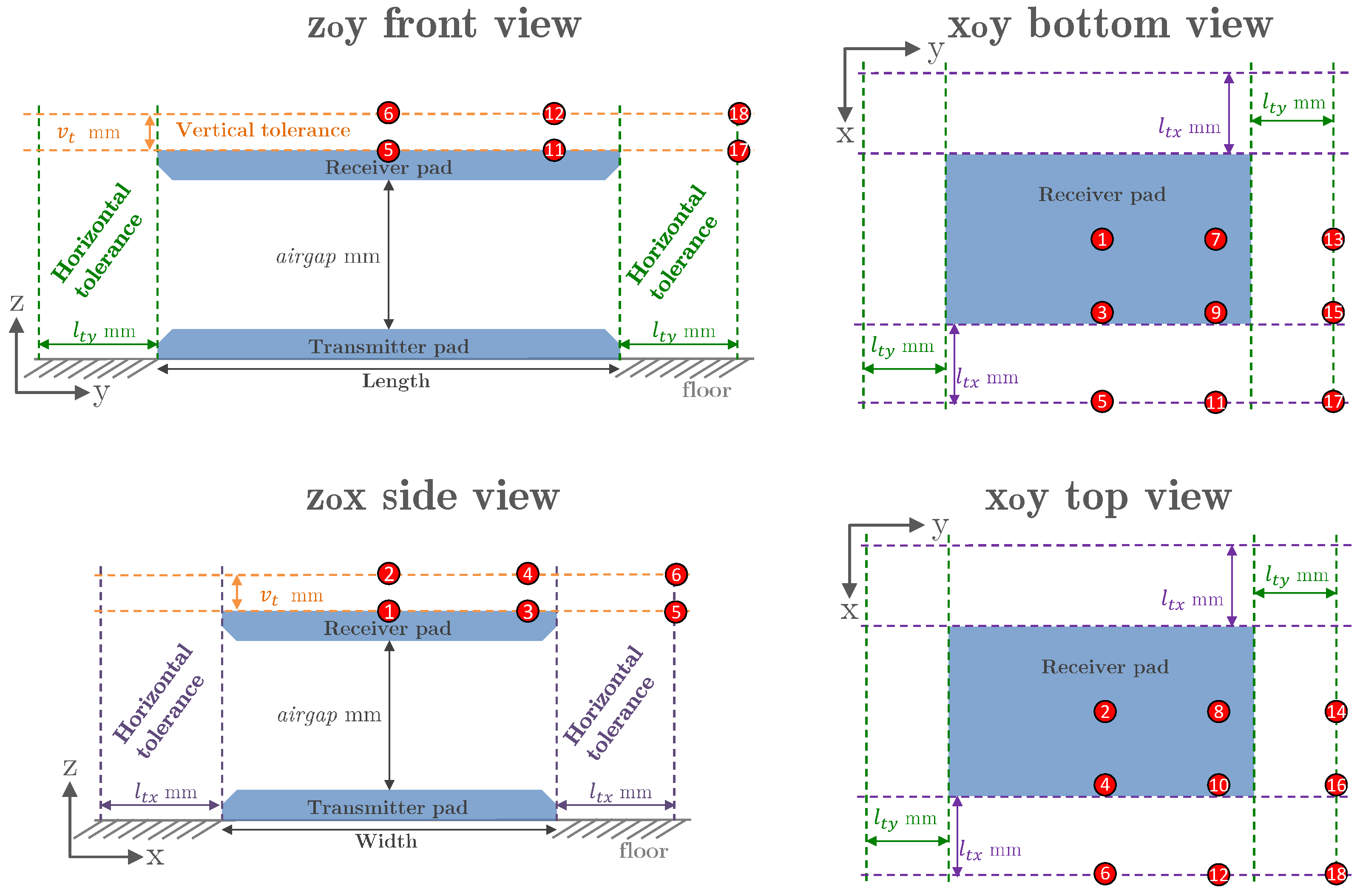
Figure 5 shows the operation area of an IPT system seen from different observation planes. The characterization of $L_{xy}=f(airgap,l_{tx},l_{ty})$ is made with the FEA results from specific $Pos$, identified in Figure 5 with red numbered circles between 1 and 18. Circular-shaped MCs only need six $Pos$, e.g., $Pos$ 1 to $Pos$ 6, as depicted in $z_{o}x$ side view. The remaining twelve $Pos$ are a consequence of different lateral displacements along the x and y axes in non-circular shaped MCs, such as the BPP. The profiling of $L_{xy}$ as a function of the turns increases the total number of FEA simulations by a factor that corresponds to the number of $Scenarios$. For example, the CP requires only one FEA simulation result in each $Pos$ if the number of turns is known. On the other hand, if the number of turns is unknown, the number of FEA simulation results in each $Pos$ increases from 1 to 4, which corresponds to the number of $Scenarios$. In short, after identifying the $Scenarios$ and $Pos$, the following approach is applied:

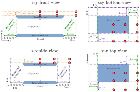
Figure 5. Operation area of the magnetic coupler.

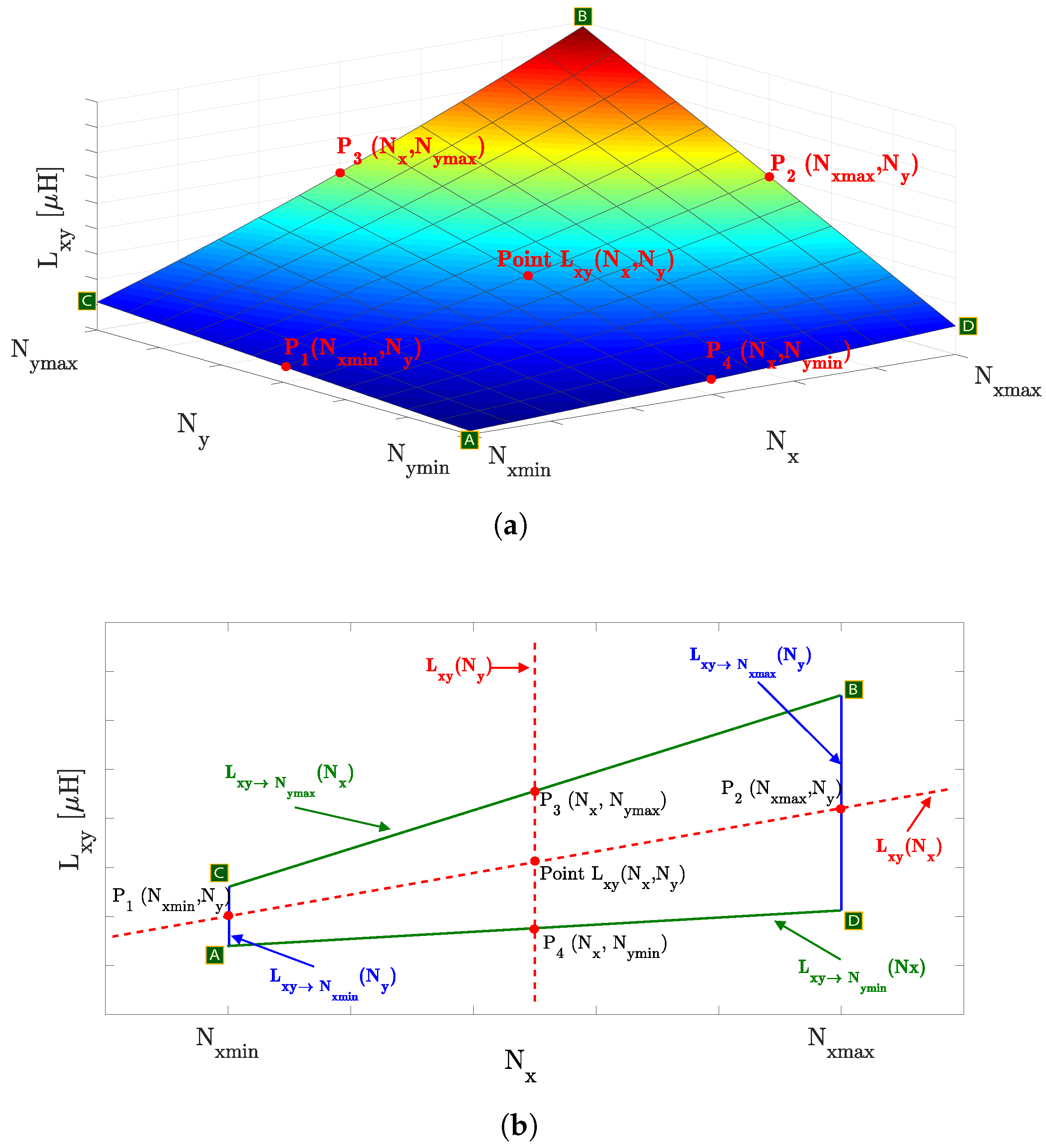
• Profile of ${\mathit{L}}_{\mathit{xy}}=\mathit{f}({\mathit{N}}_{\mathit{x}},{\mathit{N}}_{\mathit{y}})$: Figure 6 illustrates the surface of $L_{xy}=f(N_x,N_y)$ with a fixed value of $airgap$ and $l_t$, using the FEA results from $Scenario$ A to $Scenario$ D, identified by the alphabetic numbered green squares. Figure 6b depicts a 2D plane, view from the $N_x$ axis of Figure 6a. The value of $L_{xy}$ for specific values of $N_x$ and $N_y$, exemplified by the red dot labeled as $Point{L}_{xy}$ in Figure 6b, can be identified by either linear functions $L_{xy}\left(N_x\right)$ or $L_{xy}\left(N_y\right)$, illustrated by the red dashed lines, which intersect at the desired $L_{xy}$ value. The slope and intercept of $L_{xy}\left(N_x\right)$ are determined using points $P_1$ and $P_2$. The values of $P_1$ and $P_2$ are obtained using line equations $L_{x{y}_{\to N_{xmin}}}\left(N_y\right)$ and $L_{x{y}_{\to N_{xmax}}}\left(N_y\right)$ for the desired $N_y$, respectively. The desired value of $L_{xy}$ is then found using equation $L_{xy}\left(N_x\right)$ for the desired $N_x$. This process is repeated $(N_{xmax}-N_{xmin})\ast (N_{ymax}-N_{ymin})$ times to create the surface illustrated in Figure 6a. The profiling of $L_{xy}=f(N_x,N_y)$ is replicated for all charging positions $Pos$.
  

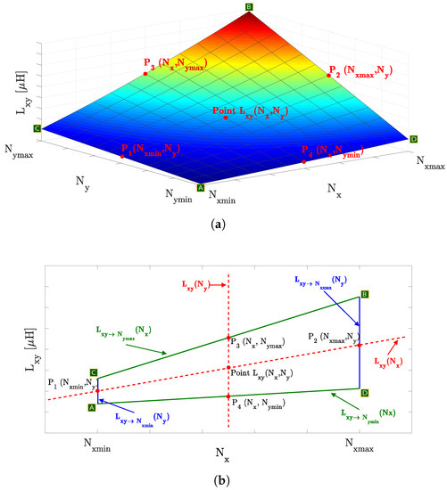  Figure 6. $L_{xy}$ as a function of $N_1$ and $N_2$ in 3D view (a) and $N_1$ axis side view (b).
• Replace $N_x$ and $N_y$ with desired values in surface function $L_{xy}=f(N_x,N_y)$, determined in step 1, and repeat the process for all simulated $Pos$. The new values of $L_{xy}$ already take into consideration the effect of the selected set of turns.
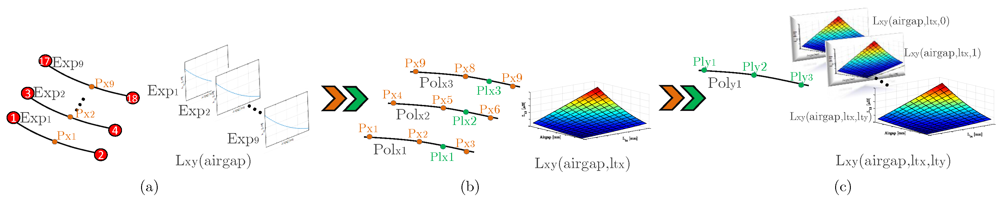
• Profile of ${\mathit{L}}_{\mathit{xy}}=\mathit{f}\left(\mathit{airgap}\right)$: Use the values found in Step 2 for $Pos$ 1 and $Pos$ 2 to determine the constants $a_1$ and $b_1$ in (7). Repeat the process for the remaining $Pos$ with the same lateral displacements but different air gap values, i.e., ($Pos$ 3, $Pos$ 4), ($Pos$ 5, $Pos$ 6), …, ($Pos$ 17, $Pos$ 18). A total of three equations are determined for circular-shaped MCs and nine equations for non-circular MCs. The equations are identified from $Exp1$ to $Exp9$ in Figure 7a.
  

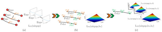  Figure 7. Step by step illustration of the fitting methodology for (a) $L_{xy}=f\left(airgap\right)$, (b) $L_{xy}=f(airgap,l_{tx})$ and (c) $L_{xy}=f(airgap,l_{tx},l_{ty})$.
• Replace $airgap$ in equations $Exp1$ to $Exp9$ with the desired value to determine $L_{xy}$ in points $P_{x1}$ to $P_{x9}$, as illustrated in Figure 7a. The new $L_{xy}$ values take into account the effect of the selected set of turns and air gap values.
• Profile of ${\mathit{L}}_{\mathit{xy}}=\mathit{f}\left({\mathit{l}}_{\mathit{tx}}\right)$: Use the values found in Step 4 that have the same $airgap$ and $l_{ty}$ values, such as $P_{x1}$ to $P_{x3}$, to determine the Gaussian constants $a_2$, $b_2$ and $c_2$ in (8). Repeat the process (if applicable) for the set of points $P_{x4}$ to $P_{x6}$ and $P_{x7}$ to $P_{x9}$. A total of one or three equations is determined according to the shape of the MC. Circular-shaped MCs are only evaluated in relation to $l_{tx}$ or $l_{ty}$ and only one equation is needed, whereas the remaining MCs require a total of three equations. Figure 7b illustrates the labeled equations from $Po{l}_{x1}$ to $Po{l}_{x3}$.
• Replace $l_{tx}$ in equations $Po{l}_{x1}$ to $Po{l}_{x3}$ with the desired value to determine $L_{xy}$ in the points $P_{lx1}$ to $P_{lx3}$, represented in Figure 7b with the color green. The new $L_{xy}$ values already take into account the effect of $N_x$, $N_y$, $airgap$ and $l_{tx}$.
• Profile of ${\mathit{L}}_{\mathit{xy}}=\mathit{f}\left({\mathit{l}}_{\mathit{ty}}\right)$: Use the values found in Step 6 to determine the Gaussian constants $a_2$, $b_2$ and $c_2$ in (8). The new function is identified as $Po{l}_{y1}$, and it is illustrated in Figure 7c.
• Replace $l_{ty}$ in equation $Po{l}_{y1}$ with the desired value to determine $L_{xy}$ for a set of turns, $airgap$, $l_{tx}$ and $l_{ty}$ values. Steps 7 and 8 are only required for non-circular shaped MCs.
• Profile of ${\mathit{L}}_{\mathit{xy}}=\mathit{f}({\mathit{N}}_{\mathit{x}},{\mathit{N}}_{\mathit{y}},\mathit{airgap},{\mathit{l}}_{\mathit{tx}},{\mathit{l}}_{\mathit{ty}})$: Repeat Step 2 to Step 8 for every combination of $N_x$, $N_y$, $airgap$, $l_{tx}$ and $l_{ty}$ to create the volume illustrated in Figure 4.

3.2. Self-Inductance Profiling

The self-inductance ($L_x$) of a coil corresponds to the quadratic number of turns ($N_x$) divided by the equivalent reluctance (ℜ), as described in (11). Variations in $N_x$ impact the value of $L_x$ directly, while $airgap$ and $l_t$ variations affect ℜ and, consequently, $L_x$. Figure 8a shows the behavior of $L_x$ as a function of $N_x$. As expected from (11), the pattern of $L_x$ follows a quadratic function, and the permeance ($1/\Re$) can be found using three FEA simulation results with different values of $N_x$:

$$L_x=\frac{N_x^2}{\Re },x=1,2,$$

(11)

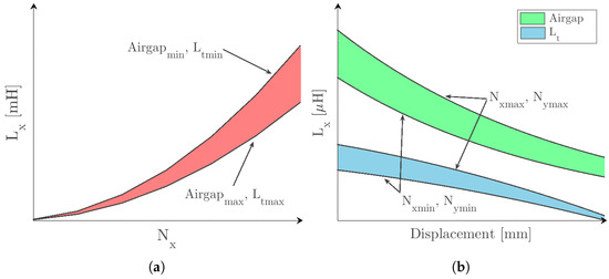
Figure 8. Profiles of $L_x$ as a function of $N_x$ (a), $airgap$ and $l_t$ (b).

However, in the scenarios A to D, listed in (10), only two different values for $N_x$, $N_{x_{min}}$ and $N_{x_{max}}$, are used. An additional scenario with a different set of turns is then needed, and it is given by:

$$ScenarioE\to N_x=N_{x_{mean}},N_y=N_{y_{mean}},$$

(12)

where $N_{x_{mean}}$ is the mean value between $N_{x_{min}}$ and $N_{x_{max}}$, and $N_{y_{mean}}$ is the mean value between $N_{y_{min}}$ and $N_{y_{max}}$.

The air gap and lateral displacements change the value of ℜ due to the presence and/or absence of ferromagnetic material from the opposite side pad. Figure 8b shows the impact displacements in $L_x$ for different $airgap$ and $l_t$ values. Charging positions with smaller $airgap$ values and $l_t=0$ have higher values of $L_x$. However, in the event of lateral displacements, the variation in $L_x$ is steeper when compared with charging positions at higher $airgap$ values. The patterns of $L_x$ as a function of $airgap$ and $l_t$ are identical to $L_{xy}$; thus, the method described in Section 3.1 can be adapted to determine $L_x=f(N_x,airgap,l_{tx},l_{ty})$ as follows:

• Profile of ${\mathit{L}}_{\mathit{x}}=\mathit{f}\left({\mathit{N}}_{\mathit{x}}\right)$: Use the FEA simulation results from $Scenario$A to $Scenario$ E, identified in (10) and (12), to determine the permeance $1/\Re$ in (11). Repeat the process for all $Pos$. A total of six equations are found for circular-shaped MCs and eighteen equations for non-circular-shaped MCs;
• Replace $N_x$ with the desired value equation $L_x=f\left(N_x\right)$, determined in step 1, and repeat the process for the remaining equations. The new values of $L_x$ already take into consideration the effect of the selected number of turns;
• Profile of ${\mathit{L}}_{\mathit{x}}=\mathit{f}({\mathit{N}}_{\mathit{x}},\mathit{airgap},{\mathit{l}}_{\mathit{tx}},{\mathit{l}}_{\mathit{ty}})$: Replicate Step 3 to Step 9 of the methodology described in Section 3.1 to model the effect of air gap and lateral displacements in $L_x$.

The aforementioned methodology profiles $L_x=f(N_x,airgap,l_{tx},l_{ty})$ through the use of FEA simulations. Some physical aspects such as the coil shape, the number of winding layers and the wire characteristics (solid or stranded) may change the self-inductance value. These physical aspects are, however, taken into account by the FEA tool in the calculus of the self-inductance values, which are then used by the proposed fitting approach. Furthermore, the profile of the self-inductance as a function of $airgap$, $l_t$ and $N_x$ still follows the patterns identified in Figure 8. In conclusion, the proposed fitting approach can be applied to coils with different shapes wounded as single-layer or multi-layer winding.

3.3. Development to Three-Coil Systems

The intermediate coil in three-coil IPT systems produces two additional mutual inductance values: $L_{32}$ and $L_{13}$. As described earlier, the profiles of $L_{12}$ and $L_{32}$ are identical and only differ by a scale factor. As for $L_{13}$, since both transmitter and intermediate coils are installed in the same enclosure that forms the transmitter pad, its value is almost independent of the air gap and lateral displacements. The effect off the number of turns, on the other hand, is the same as $L_{12}$ and $L_{32}$, and it can be obtained using Step 1 of the proposed approach (Profile of $L_{xy}=f(N_x,N_y)$). However, the $Scenarios$ listed in (10) are not sufficient to characterize $L_{12}$, $L_{32}$ and $L_{13}$ as a function of the number of turns. The new set of scenarios is given by:

$$\begin{array}{cc}\hfill ScenarioA& \to N_1=N_{1_{min}},N_2=N_{2_{min}},N_3=N_{3_{min}}\hfill \\ \hfill ScenarioB& \to N_1=N_{1_{max}},N_2=N_{2_{max}},N_3=N_{3_{max}}\hfill \\ \hfill ScenarioC& \to N_1=N_{1_{min}},N_2=N_{2_{max}},N_3=N_{3_{min}}\hfill \\ \hfill ScenarioD& \to N_1=N_{1_{max}},N_2=N_{2_{min}},N_3=N_{3_{max}}\hfill \\ \hfill ScenarioE& \to N_1=N_{1_{mean}},N_2=N_{2_{mean}},N_3=N_{3_{mean}}\hfill \\ \hfill ScenarioF& \to N_1=N_{1_{min}},N_2=N_{2_{max}},N_3=N_{3_{max}}\hfill \\ \hfill ScenarioG& \to N_1=N_{1_{max}},N_2=N_{2_{min}},N_3=N_{3_{min}}\hfill \end{array}$$

(13)

where $N_3$ is the number of turns in the intermediate coil, and $N_{3_{min}}$, $N_{3_{mean}}$ and $N_{3_{max}}$ correspond to the minimum, mean and maximum number of turns, respectively. The results from scenarios A to D characterize $L_{12}$ and $L_{32}$ while scenarios A, B, F and G characterize $L_{13}$ as a function of the number of turns. Scenario E is used in the profiling of $L_x$, described in Section 3.2.

4. Case Study

This section validates the proposed approach, step-by-step, using the FLCP for a particular set of turns and in a specific charging position. Then, a prototype is built and the mapping profile of self and mutual inductances is validated experimentally under different vertical and lateral displacements. Estimation errors and computational time gains of the proposed mapping methodology are evaluated and compared with existing literature.

4.1. Specifications and FEA Simulations

Table 1 presents the operation specifications and some physical constraints of a typical IPT application. The installation area hinges the MC geometry, and it imposes, inadvertently, the lateral tolerance limits and maximum size for the MC. On the other hand, the minimum admissible size for the MC depends on system specifications such as output power levels, air gap and lateral displacement values. One characteristic of non-polarized pads is the total decoupling between the transmitter and receiver pads when the lateral displacements exceed around 40% of the total diameter (d) of the pads [1]. This means the FLCP needs a minimum size of 400 mm to comply with the lateral tolerance of 150 mm, listed in Table 1. An FLCP with a size of 650 mm was selected for evaluation, and it respects the maximum size limit of 800 mm imposed by Table 1. The transmitter and receiver pads of FLCP have the same size, and its dimensions are shown in Figure 2b.

Table 1. System specifications and physical constraints.

Specifications and Constraints	Value
Normal frequency operation ($f_s$)	85 kHz
$airgap$	[100–250 mm]
lateral tolerance ($l_t$)	[0–150 mm]
Maximum $|{\overline{I}}_1|$, $|{\overline{I}}_2|$, $|{\overline{I}}_3|$	30 A
Maximum MC size ($length$)	800 mm

The coils are wounded with Litz wire formed by 1050 strands, a cross-section of 4 mm${}^2$ and a rated current of 30 A. The value of $N_{x_{min}}$ is set at 2, whereas $N_{x_{max}}$ is set at 14 in order to avoid large induced voltage values at the coil terminals. The ferromagnetic core is modeled with the characteristics of the material N87 from Epcos.

A 3D model of the FLCP was created and simulated in an FEA tool called Flux from Altair. Each simulation has a second-order mesh with approximately 40,000 mesh nodes. The use of a second-order mesh increases the simulation time, but it provides accurate results, especially in ferrite-less geometries, such as the FLCP. The open-circuit test is performed in each coil, and the mutual and self-inductance values are determined using (2) and (3), respectively. This means that the same $Scenario$ in each $Pos$ has to be simulated with three different electric circuits. The total number of FEA simulations needed for a full characterization of an MC is then determined by:

$$N_{sim}=N_{Scenario}·N_{Pos}·N_{coil},$$

(14)

where $N_{coil}$ is the total number of coils in the MC, and it can take the values 2 or 3 for two- or three-coil systems, respectively. The parameters $N_{Scenario}$ and $N_{Pos}$ correspond to the total number of required $Scenarios$ and $Pos$, respectively. Table 2 lists the minimum number of simulations required for different MCs based on (14).

Table 2. Minimum number of required FEA simulations needed to profile the self- and mutual-inductance.

${\mathit{N}}_{\mathit{x}}$known
MC	${\mathit{N}}_{\mathit{Pos}}$	$\mathit{Scenario}$	${\mathit{N}}_{\mathit{coil}}$	${\mathit{N}}_{\mathit{sim}}$
CP	6	1	2	12
BPP	18	1	2	36
FLCP	6	1	3	18
${\mathit{N}}_{\mathit{x}}$unknown
CP	6	5	2	60
BPP	18	5	2	180
FLCP	6	7	3	126

The runtime of each simulation ranges from 7 to 15 min, using a computer with an i7 4960X processor (max frequency of 4.00 GHz), 32 GB DDR3 at 2133 MHz and 2 TB HDD 7200 RPM Sata disk.

4.2. Self and Mutual Inductance Profiling

This section explains in detail how to obtain the value of $L_{12}$ and $L_1$ for an $airgap=185$ mm and $l_t=100$ mm of the FLCP with 650 mm. As identified in Section 3.3, the FLCP and CP require the simulation results in six $Pos$ ($N_{Pos}=6$) to extrapolate the mutual and self-inductance profiles. Since the number of turns is unknown, a total of seven $Scenarios$ ($N_{Scenario}=7$), identified in (13), have to be simulated for each $Pos$. A total of 126 FEA simulations, according to (14), are then needed to extract the mutual and self-inductance values. The charging positions are illustrated in the $zox$ side view of Figure 5, and they have the following coordinates: ($airgap$, $l_t$): $Pos$ 1 = (100, 0), $Pos$ 2 = (250, 0), $Pos$ 3 = (100, 75), $Pos$ 4 = (250, 75), $Pos$ 5 = (100, 150) and $Pos$ 6 = (250, 150).

Table 3 lists the FEA simulation results from $Scenarios$ A to E, described in (13), in each $Pos$ for the FLCP with a size of 650 mm. The first step in the fitting approach method is the identification of $L_{12}=f(N_1,N_2)$ in all six $Pos$. The method described in Section 3.1.1 is applied in detail to $Pos$ 1. Figure 9 illustrates $L_{12}=f(N_1,N_2)$ in a 2D view for $Pos$ 1 with all significant values. The corners of the geometric figure correspond to the $L_{12}$ values of $Scenario$ A to $Scneario$ D. The linear function between $Scenario$ A and $Scenario$ D corresponds to a fixed value of two turns ($N_{2min}$) in the receiver coil, while the number of turns of the transmitter is varied, and it is given by:

$$L_{12\to N_{2min}}\left(N_1\right)=0.613\times {10}^{-6}·N_1-0.107\times {10}^{-6}.$$

(15)

Table 3. FEA simulation results of all $Scenarios$ in each $Pos$ for the 650 mm FLCP.

Scenarios	A		B		C		D		E		Unit
	${\mathit{L}}_{\mathbf{12}}$	${\mathit{L}}_{\mathbf{1}}$	${\mathit{L}}_{\mathbf{12}}$	${\mathit{L}}_{\mathbf{1}}$	${\mathit{L}}_{\mathbf{12}}$	${\mathit{L}}_{\mathbf{1}}$	${\mathit{L}}_{\mathbf{12}}$	${\mathit{L}}_{\mathbf{1}}$	${\mathit{L}}_{\mathbf{12}}$	${\mathit{L}}_{\mathbf{1}}$
$Pos$ 1	1.12	4.32	66.2	160	8.4	4.33	8.48	161	19.9	56.8	[$\mathsf{\mu }$H]
$Pos$ 2	0.34	4.23	21.9	155	2.7	4.23	2.73	155	6.3	55.3
$Pos$ 3	0.95	4.31	57.6	159	7.28	4.3	7.36	159	17.1	56.5
$Pos$ 4	0.31	4.22	20.4	155	2.51	4.23	2.53	155	5.84	55.2
$Pos$ 5	0.63	4.26	40.2	157	5.02	4.27	5.03	157	11.6	55.9
$Pos$ 6	0.24	4.22	16.5	155	1.99	4.22	2.01	155	4.63	55.3

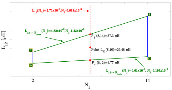
Figure 9. Profile of $L_{12}=f(N_1,N_2)$ in a 2D view for $Pos$ 1.

The constants in (15) are found using a curve-fitting tool, such as the fit command in Matlab. The fitting process of two-dimensional functions, such as linear, exponential or Gaussian functions, requires the x- and y-point coordinates in two separate vectors. The curve-fitting tool then applies linear or nonlinear parametric regression to the inserted vectors, and it retrieves the respective constants. For example, the x and y vectors used in (15) were $[2,14]$ and [1.12 × 10${}^{-6}$, 8.48 × 10${}^{-6}$], respectively. The x vector corresponds, in this particular case, to the values of $N_1$ in $Scenario$ A and $Scenario$ D, whereas the y vector is the correspondent $L_{12}$ values in the same $Scenarios$. The same approach is also applied to discover the constant values in exponential and Gaussian functions.

Analogously, the linear function between $Scenario$ C and $Scenario$ B corresponds to a fixed value of 14 turns ($N_{2max}$) in the receiver coil while the number of turns of the transmitter is varied according to:

$$L_{12\to N_{2max}}\left(N_1\right)=4.82\times {10}^{-6}·N_1-1.23\times {10}^{-6}$$

(16)

All admissible $L_{12}$ values for every combination of $N_1$ and $N_2$ are in between Equations (15) and (16). To validate the methodology that finds $L_{12}$ for a particular set of turns, the following conditions are assumed as an example: $N_1=8$ and $N_2=10$. First, the $L_{12}$ values for points $P_3$ and $P_4$ are determined by replacing $N_1$ with the value 8 in (16) and (15), respectively. The impact of $N_1$ is already taken into account in $P_3$ and $P_4$ for $N_{2max}$ and $N_{2min}$, respectively. The linear function between $P_3$ and $P_4$ infers the impact of $N_2$ in $L_{12}$, defined as:

$$L_{12}\left(N_2\right)=2.71\times {10}^{-6}·N_2-0.618\times {10}^{-6}.$$

(17)

The value $L_{12}$ = 26.5 $\mathsf{\mu }$H for $Pos$ 1 is finally determined using (17) and replacing $N_2$ with 10. The same approach is applied to the remaining five $Pos$, and the results are listed in Table 4

Table 4. Estimation results of $L_{12}$ in all six $Pos$ for $N_1=8$ and $N_2=10$.

Pos 1	Pos 2	Pos 3	Unit
$L_{12}=26.48$	$L_{12}=8.71$	$L_{12}=23.01$	$\mathsf{\mu }$H
Pos4	Pos5	Pos6
$L_{12}=8.11$	$L_{12}=16.02$	$L_{12}=6.5$	$\mathsf{\mu }$H

Step 2 of the fitting approach method characterizes $L_{12}=f(airgap,l_t)$ using the values found in Step 1 for a particular set of turns. The estimated results of $L_{12}$ for $N_1=8$ and $N_2=10$, listed in Table 4, are used as an example to validate Step 2 of the proposed approach in detail. First, $L_{12}$ is characterized as a function of the $airgap$ for $Pos$ with the same $l_t$. The $L_{12}$ results for $Pos$ 1 and $Pos$ 2, identified in Table 4, are inserted in a curve-fitting tool to discover the constant values in (7). In this particular case, the x vector used in fitting tool is equal to $[100,250]$, whereas the y vector is equal to $[26.48\times {10}^{-6},8.71\times {10}^{-6}]$. The same approach is carried out for the $L_{12}$ pair results ($Pos$ 3, $Pos$ 4) and ($Pos$ 5, $Pos$ 6), and they are defined as:

$$\begin{array}{cc}\hfill L_{{12}_{Px1}}\left(airgap\right)& =55.5\times {10}^{-6}·e^{\left(-7.41\times {10}^{-3}·airgap\right)}\hfill \\ \hfill L_{{12}_{Px2}}\left(airgap\right)& =46.1\times {10}^{-6}·e^{\left(-6.95\times {10}^{-3}·airgap\right)}\hfill \\ \hfill L_{{12}_{Px3}}\left(airgap\right)& =29.1\times {10}^{-6}·e^{\left(-5.97\times {10}^{-3}·airgap\right)}.\hfill \end{array}$$

(18)

To determine $L_{12}$ at a particular air gap value, the variable $airgap$ is replaced in (18) by the desired value. Therefore, these three exponential equations determine three new $L_{12}$ values in specific charging positions, labeled from $P_{x1}$ to $P_{x3}$. As an example, the $airgap$ in (18) is replaced by 185 mm, and the following $L_{12}$ values are found: $L_{{12}_{Px1}}$ = 14.1 $\mathsf{\mu }$H, $L_{{12}_{Px2}}$ = 12.74 $\mathsf{\mu }$H and $L_{{12}_{Px3}}$ = 9.64 $\mathsf{\mu }$H. These $L_{12}$ values are valid for $N_1=8$, $N_2=10$ and $airgap=185$ mm, with lateral displacements of 0, 75 and 150 mm, respectively. The remaining values of $L_{12}$ for charging positions with different lateral displacements are found using (8). The constants in (8) are obtained with the curve-fitting tool, using the values of $L_{12}$ from $P_{x1}$ to $P_{x3}$. The vectors used in the fitting tool were $x=$ [0, 75, 150] and $y=[14.1\times {10}^{-6},12.74\times {10}^{-6},9.64\times {10}^{-6}]$, respectively. The new equation, described in (19), determines $L_{12}$ value as a function of $l_t$ for an FLCP with a size of 650 mm:

$$L_{12}\left(l_t\right)=14.08\times {10}^{-6}·e^{-{((l_t+111.4\times {10}^{-19})/2.043)}^2}.$$

(19)

To find $L_{12}$ in a particular lateral displacement, the variable $l_t$ is replaced in (19) with the desired value. As an example, $l_t$ was replaced by 100 mm, and the value of $L_{12}=11.78$ $\mathsf{\mu }$H was found.

The aforementioned process determined the specific value of $L_{12}$ for $N_1=8$, $N_2=10$, $airgap=185$ mm and $l_t=100$ mm, but the proposed approach extends beyond the estimation of $L_{12}$ in a particular set of conditions. For instance, the results illustrated in Figure 9 show the profile of $L_{12}=f(N_1,N_2)$ in $Pos$ 1, and it allows the immediate extrapolation of $L_{12}$ for all possible combinations of turns without additional FEA simulations. Furthermore, the exponential equations, listed in (18), characterize $L_{12}$ for a particular set of turns and as a function of $airgap$, and they extrapolate $L_{12}$ for different air gap values, even those that are outside the specifications listed in Table 1. In conclusion, the proposed approach profiles $L_{12}$ individually as a function of different parameters, and it combines all individual profiles in an iterative way to form, ultimately, the volume of $L_{12}$ shown in Figure 4.

Concluding the validation process of the mutual inductance, the proposed approach is now applied to the self-inductance. The profiling of $L_1$ is explained step-by-step as a guide reference, but the same fitting methodology extends to $L_2$ and $L_3$. As described in Section 3.2, the first step in profiling $L_1=f(N_1,airgap,l_t)$ is the identification of $L_1=f\left(N_1\right)$ in all $Pos$. The $L_1$ results from $Scenarios$ A, B and E, listed in Table 3, are inserted in the curve-fitting tool to find the constants of a second-order polynomial function, given by (11). A total of six equations are found for the $Scenario$ results of $Pos$ 1 to $Pos$ 6. The equations found for $Pos$ 2, $Pos$ 4 and $Pos$ 6 are described in (20), and they were selected to show the impact of lateral displacement in $L_1$:

$$\begin{array}{cc}\hfill L_{1_{Pos2}}\left(N_1\right)& =803\ast {10}^{-9}·N_1^2\hfill \\ \hfill L_{1_{Pos4}}\left(N_1\right)& =802\ast {10}^{-9}·N_1^2\hfill \\ \hfill L_{1_{Pos6}}\left(N_1\right)& =803\ast {10}^{-9}·N_1^2.\hfill \end{array}$$

(20)

As can be observed, the quadratic constants across all equations in (20) are similar, and they correspond to the permeance of the transmitter pad. These results indicate that the presence of the receiver pad has small impact in the magnetic flux distribution of the transmitter pad, within the evaluated air gap and lateral displacement values. The value of $L_1$ for a particular $N_1$ is found by replacing $N_1$ in the corresponding second-order polynomial equations of each $Pos$. As an example, the value of $N_1=10$ was assumed and the estimated $L_1$ values are listed in Table 5. The results show a maximum deviation of 3.2% between the minimum and maximum values, and they are in line with the existing literature. Nevertheless, the impact of the air gap and lateral displacements must be accounted for using the same approach as the identification of $L_{12}=f(airgap,l_t)$. The set of $L_1$ results in the same lateral displacements, i.e., the set of $L_1$ values ($Pos$ 1, $Pos$ 2), ($Pos$ 3, $Pos$ 4) and ($Pos$ 5, $Pos$ 6) are used to find the constants in (7). These exponential equations model $L_1$ as a function of the air gap in three distinct lateral displacement values. As an example, using the same $airgap$ value of 185 mm, the following $L_1$ values are found in the specific charging positions: $L_{1_{Px1}}$ = 81.4 $\mathsf{\mu }$H, $L_{1_{Px2}}$ = 81.2 $\mathsf{\mu }$H and $L_{1_{Px3}}$ = 80.8 $\mathsf{\mu }$H.

Table 5. Estimation results of $L_1$ in all six $Pos$ for $N_1=10$.

Pos 1	Pos 2	Pos 3	Unit
$L_1=82.9$	$L_1=80.3$	$L_1=82.4$	$\mathsf{\mu }$H
Pos4	Pos5	Pos6
$L_1=80.3$	$L_1=81.4$	$L_1=80.3$

To account for the effect of lateral displacements, the obtained values of in $L_1$ in $P_{x1}$, $P_{x2}$ and $P_{x3}$ are used to find the constants in (8) through a curve-fitting tool. The new function characterizes $L_1$ as a function of $l_t$ for an $airgap=185$ mm and $N_1=10$. The variable $l_t$ is then replaced with the desired value to find the final value for $L_1$. The process is repeated iteratively to build the profile $L_1=f(N_1,airgap,l_t)$. The same approach is conducted for $L_2$ and $L_3$.

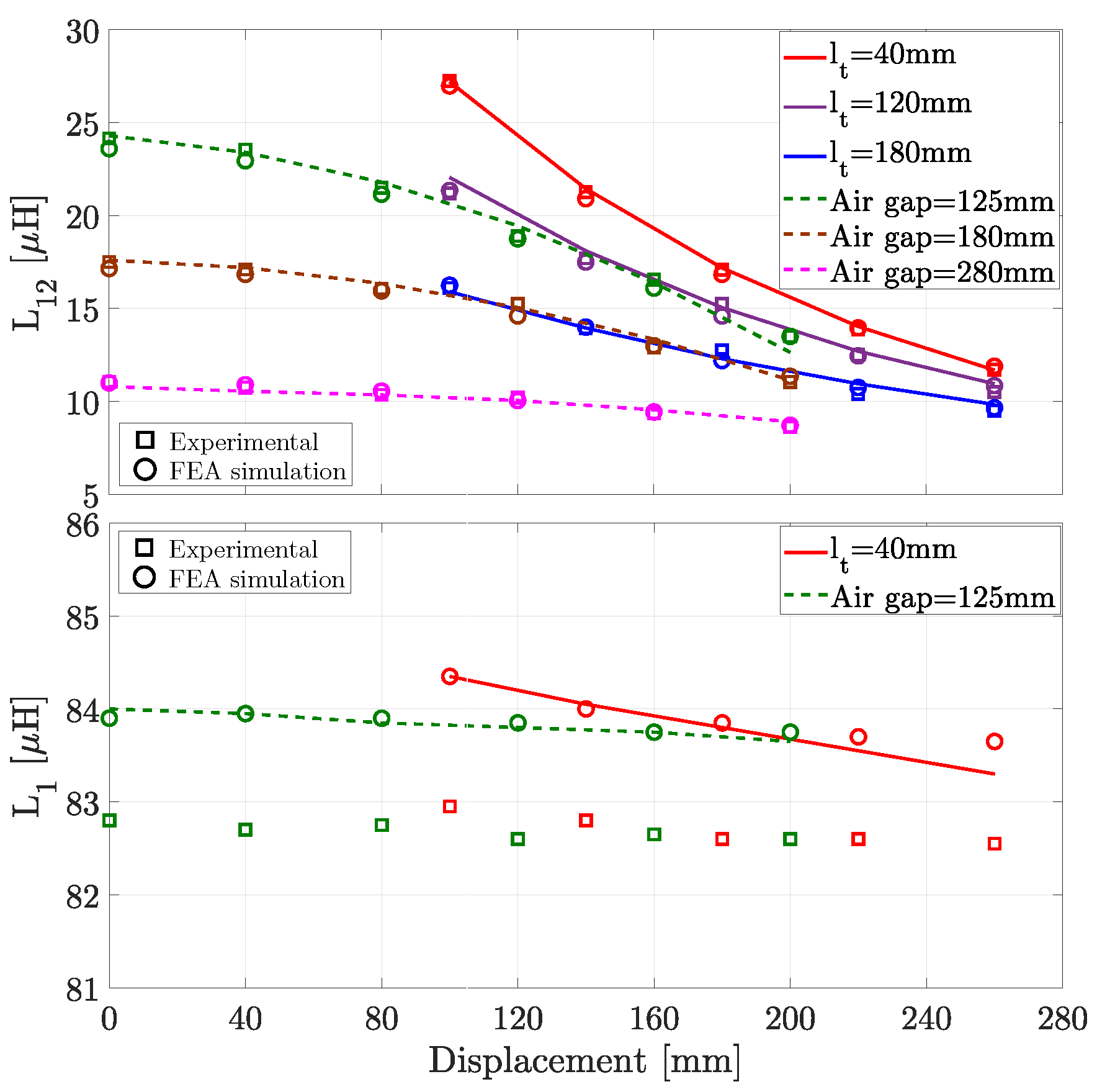
Figure 10a illustrates the built prototype of a FLCP and test bench. A detailed view of both the transmitter and receiver pads is made in Figure 10b with the following turns: $T_1=10$, $T_2=14$ and $T_3=6$. The FEA simulation results from Table 3 were used to extrapolate the fitting curves of $L_{12}$ and $L_1$, illustrated in Figure 11. For each solid line, $l_t$ is constant and the $airgap$ is varied. As such, the x axis corresponds to the vertical displacements. For dashed lines, the analysis is reversed, i.e., the $airgap$ is constant and $l_t$ is varied along the x axis. The experimental measurements correspond to square points, and the FEA simulations correspond to circle points. From the figure analysis, it is possible to confirm that both Gaussian and exponential decay functions can be used to mimic the behavior for $L_{12}$ and $L_1$. Fitting-based methods have inherent estimation errors that depend on the numbers, quality and distance between the fitting points. Any difference can be mitigated by adjusting the fitting parameters of the curve-fitting tool to reduce the square errors in the worst charging positions, i.e., for the highest vertical and lateral displacements.

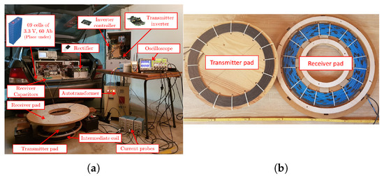
Figure 10. Experimental prototype built in a converted combustion vehicle: (a) Main overview and (b) transmitter and receiver pads.

Figure 11. Comparison of the fitting approach with both experimental and FEA simulation data as a function of both vertical and lateral displacements.

4.3. Performance and Runtime

The estimation discrepancies of the proposed fitting approach method against FEA simulations and experimental data are quantified in this subsection as well as the time savings by the proposed mapping approach with the existing literature.

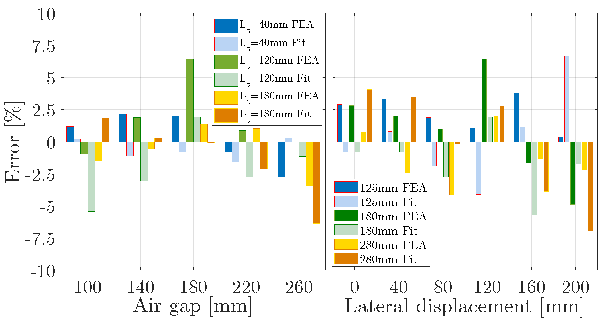
Figure 12 lists the errors between the fitting curves, the experimental data and FEA simulation results for $L_{12}$ under vertical and lateral displacements. Within feasible displacements, the average error between the experimental data and the proposed fitting is below 3%. The error difference is higher in scenarios where the value of $l_t$ is higher. For example, a charging position outside the displacement specifications listed in Table 1 (($airgap$, $l_t$) = (280, 200 mm)), corresponding to a coupling factor of 0.06, has an error of 6.8% between experimental and fitting curve (0.58 $\mathsf{\mu }$H). The estimation errors are higher (between 4.2 and 7%) for charging scenarios that exhibit low coupling values (between 0.04 and 0.078). Such charging positions are unfeasible for an efficient high-throughput energy transfer due to the high circulating currents required in the transmitter side. Similar error results are found for $L_{23}$, and for that reason, they are not displayed.

Figure 12. Errors between the experimental data and both FEA simulations and fitting approach methodology.

The estimation errors for $L_1$ are between 2.4 and 3.2%. This error range is a consequence of an 1.4 $\mathsf{\mu }$H offset between the experimental data and the fitting approach and FEA simulation results, as depicted in the second graph of Figure 11. Despite the offset value, the fitting curves follow the same pattern of the experimental data. Similar $L_1$ values are obtained in different vertical and lateral displacements with difference errors in the range of 0.8 to 3.4%.

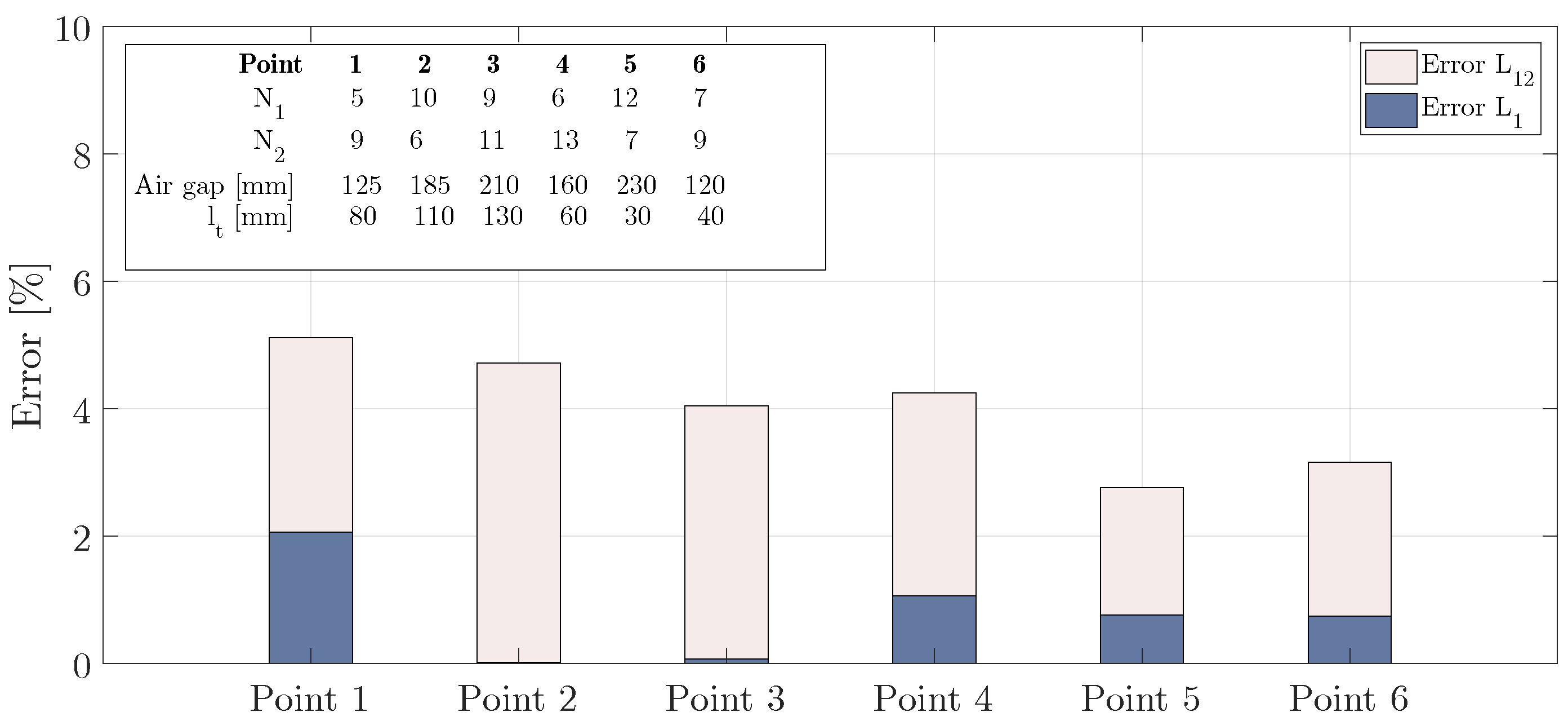
Figure 13 shows the error results between the fitting approach method and 3D FEA simulation results for $L_1$ and $L_{12}$ with an FLCP size of 650 mm. The comparison is made with the FLCP in six different charging positions and with different sets of turns, as identified in the top left corner of Figure 13. The results show an average error in $L_{12}$ around 4%, whereas the average error of $L_1$ is inferior at 1%. The highest errors in $L_{12}$ occur for higher lateral displacement values, such as points 1 and 2. In these cases, the values of $L_{12}$ are inferior to 10 $\mathsf{\mu }$H and had a variation of just 0.5 $\mathsf{\mu }$H in the fitting approach, which lead to an error of 5%. The estimation of $L_1$, on the other hand, has average errors inferior to 1%, and in some conditions, such as point 2 and point 3, the error is negligible. This was due to the little effect of the air gap and lateral displacements in the self-inductance values, which reduces the estimation errors. Similar error results were obtained for $L_2$, $L_3$ and $L_{23}$ and for this reason are not depicted in Figure 13.

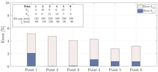
Figure 13. Estimation errors between the proposed fitting approach and FEA simulations.

One benefit of the proposed approach is the reduced number of FEA simulations required to create the self and mutual inductance profiles. Table 2 lists the minimum number of simulations required for different MCs for known and unknown $N_x$. As explained in Section 3.1, the profiling of the self and mutual inductance surfaces as a function of the number of turns requires the simulation of $Scenarios$ in each $Pos$. The final number of required simulations in the unknown category is then affected by a factor that equals the number of $Scenarios$. Furthermore, non-circular-shaped MCs require twelve additional $Pos$, such as the BPP in Table 2, to profile $L_{xy}$ and $L_x$ as a function of lateral displacements along the x and y axes. These types of MCs require a total of 180 FEA simulations, if the set of turns is unknown, and 36 FEA simulations, if the set of turns is known. On the other hand, circular designs such as the CP only require six $Pos$, and the total number of simulations is reduced to one-third when compared with the BPP. In overall, the total number of FEA simulations that fully characterize an MC are comprised between 12 (for the CP) and 180 (for the BPP).

Table 6 shows the benefits of the proposed fitting approach, taking into account the presented case study, in comparison with the typical approach. In addition, a benchmark comparison is also made in Table 6 with existing works in the literature. The table is subdivided into two groups: Literature and Proposed work. The first group shows the total number of evaluated MCs, whether the number of turns is known and the total number of simulations carried out in each work ($N_{Sim}$). The second group, identified in bold, shows the total number of simulations needed to characterize the MCs with the proposed fitting approach and the computational saving time in percentage. The first row in the table compares the profiling of the mutual and self-inductance values of the presented case study with the conventional approach and the proposed fitting methodology. To determine the number of simulations in the typical approach, the analysis of three different air gap values and five lateral displacements was established, making a total of 15 different charging positions. In terms of turns, six FLCPs were considered with different sets of turns, making a total of $N_{Sim}=3$ × 5 × 6 × $N_{coils}=270$ FEA simulations. These assumptions are in line with the existing literature to profile $L_x$ and $L_{xy}$. As can be observed, with the proposed fitting approach, for an unknown number of turns, the time savings are around $54\%$. These time savings only accounts for six different sets of turns, whereas the proposed approach takes into account all possible combination of turns between 1 and 14, which would increase the time savings by more than 90%. The remaining rows of Table 6 compare the proposed approach with the existing literature. As expected, the total number of simulations considered in works [9,16] is drastically reduced using the proposed fitting approach with time savings around 80%. Optimization works of MCs, such as [21,22], can also take advantage of the proposed fitting approach. However, the lack of information regarding the total number of simulations, the air gap and lateral displacement intervals make the time savings estimation difficult. Still, if the simulation intervals for the air gap and lateral displacements are between 25 and 50 mm, the fitting approach could reduce the total number of simulations between 20% and 50% in the aforementioned works.

Table 6. Benefits of the proposed fitting approach in the existing literature.

Literature				Proposed Work
Work	MCs	$N_x$	$N_{Sim}$	$N_{sim}$	Time Savings
*	1	unknown	270	126	≈54%
[16]	64	known	11,648	2304	≈80%
[9]	9	known	1446	336	$\approx 77$%

* Case study presented in this work.

5. Conclusions

The characterization of a magnetic coupler using only FEA tools is a time-consuming endeavor. This work presents a mapping methodology of the mutual and self-inductance profiles in magnetic couplers as a function of the number of turns, air gaps and lateral displacement values using a minimum number of FEA simulations. The methodology models the effect of vertical and lateral displacements with decay exponential and Gaussian functions, respectively. The effects of the number of turns are modeled using linear and second-order functions for mutual and self-inductance values, respectively.

The mapping methodology avoids new FEA simulations if the charging positioning or power requirements are modified. In addition, the use of fitting curves converts discrete FEA points in a continuous mapped volume. As an example, 12 FEA simulations are required to fully map the CP and 180 FEA simulations for the DDP and BPP. The proposed methodology can also be applied to MCs with an intermediate coupler. The method was compared with FEA simulations and validated experimentally with an FLCP geometry. The fitted Gaussian and exponential curves exhibit a good correlation with the experimental data, and an average error below 3% is found, even under charging conditions outside the design specifications. The computational effort and time savings of the proposed approach can be improved up to 80% when compared with the existing literature. The fitted exponential curves can, however, exhibit larger errors ( around 6%) if the air gap range is high (variations above 200 mm). This limitation can be mitigated with three or nine FEA simulation results with intermediary air gap values.

References

- Bandyopadhyay, S.; Venugopal, P.; Dong, J.; Bauer, P. Comparison of Magnetic Couplers for IPT-Based EV Charging Using Multi-Objective Optimization. IEEE Trans. Veh. Technol. 2019, 68, 5416–5429. [Google Scholar] [CrossRef]
- Bosshard, R.; Iruretagoyena, U.; Kolar, J.W. Comprehensive Evaluation of Rectangular and Double-D Coil Geometry for 50 kW/85 kHz IPT System. IEEE J. Emerg. Sel. Top. Power Electron. 2016, 4, 1406–1415. [Google Scholar] [CrossRef]
- Budhia, M.; Boys, J.T.; Covic, G.A.; Huang, C.Y. Development of a Single-Sided Flux Magnetic Coupler for Electric Vehicle IPT Charging Systems. IEEE Trans. Ind. Electron. 2013, 60, 318–328. [Google Scholar] [CrossRef]
- Zaheer, A.; Covic, G.A.; Kacprzak, D. A Bipolar Pad in a 10-kHz 300-W Distributed IPT System for AGV Applications. IEEE Trans. Ind. Electron. 2014, 61, 3288–3301. [Google Scholar] [CrossRef]
- Zhong, W.X.; Zhang, C.; Liu, X.; Hui, S.Y.R. A Methodology for Making a Three-Coil Wireless Power Transfer System More Energy Efficient Than a Two-Coil Counterpart for Extended Transfer Distance. IEEE Trans. Power Electron. 2015, 30, 933–942. [Google Scholar] [CrossRef]
- Kamineni, A.; Covic, G.A.; Boys, J.T. Analysis of Coplanar Intermediate Coil Structures in Inductive Power Transfer Systems. IEEE Trans. Power Electron. 2015, 30, 6141–6154. [Google Scholar] [CrossRef]
- Moon, S.; Kim, B.C.; Cho, S.Y.; Ahn, C.H.; Moon, G.W. Analysis and Design of a Wireless Power Transfer System with an Intermediate Coil for High Efficiency. IEEE Trans. Ind. Electron. 2014, 61, 5861–5870. [Google Scholar] [CrossRef]
- Li, Y.; Xu, Q.; Lin, T.; Hu, J.; He, Z.; Mai, R. Analysis and Design of Load-Independent Output Current or Output Voltage of a Three-Coil Wireless Power Transfer System. IEEE Trans. Transp. Electrif. 2018, 4, 364–375. [Google Scholar] [CrossRef]
- Marques, E.G.; Mendes, A.M.S. Optimization of transmitter magnetic structures for roadway applications. In Proceedings of the 2017 IEEE Applied Power Electronics Conference and Exposition (APEC), Tampa, FL, USA, 36–30 March 2017; pp. 959–965. [Google Scholar] [CrossRef]
- Jiwariyavej, V.; Imura, T.; Hori, Y. Coupling Coefficients Estimation of Wireless Power Transfer System via Magnetic Resonance Coupling Using Information from Either Side of the System. IEEE J. Emerg. Sel. Top. Power Electron. 2015, 3, 191–200. [Google Scholar] [CrossRef]
- Chow, J.P.W.; Chung, H.S.H.; Cheng, C.S. Use of Transmitter-Side Electrical Information to Estimate Mutual Inductance and Regulate Receiver-Side Power in Wireless Inductive Link. IEEE Trans. Power Electron. 2016, 31, 6079–6091. [Google Scholar] [CrossRef]
- Su, Y.; Chen, L.; Wu, X.; Hu, A.P.; Tang, C.; Dai, X. Load and Mutual Inductance Identification from the Primary Side of Inductive Power Transfer System With Parallel-Tuned Secondary Power Pickup. IEEE Trans. Power Electron. 2018, 33, 9952–9962. [Google Scholar] [CrossRef]
- Marques, E.G.; Mendes, A.M.S.; Perdigão, M.S.; Costa, V.S. Design Methodology of a Three Coil IPT System with Parameters Identification for EVs. IEEE Trans. Veh. Technol. 2021, 70, 7509–7521. [Google Scholar] [CrossRef]
- Acero, J.; Carretero, C.; Lope, I.; Alonso, R.; Lucia, Ó.; Burdio, J.M. Analysis of the Mutual Inductance of Planar-Lumped Inductive Power Transfer Systems. IEEE Trans. Ind. Electron. 2013, 60, 410–420. [Google Scholar] [CrossRef]
- Wei, G.; Jin, X.; Wang, C.; Feng, J.; Zhu, C.; Matveevich, M.I. An Automatic Coil Design Method with Modified AC Resistance Evaluation for Achieving Maximum Coil Coil Efficiency in WPT Systems. IEEE Trans. Power Electron. 2020, 35, 6114–6126. [Google Scholar] [CrossRef]
- Nagendra, G.R.; Covic, G.A.; Boys, J.T. Determining the physical size of inductive couplers for IPT EV systems. In Proceedings of the 2014 IEEE Applied Power Electronics Conference and Exposition—APEC, Fort Worth, TX, USA, 16–20 March 2014; pp. 3443–3450. [Google Scholar]
- Song, K.; Ma, B.; Yang, G.; Jiang, J.; Wei, R.; Zhang, H.; Zhu, C. A Rotation-Lightweight Wireless Power Transfer System for Solar Wing Driving. IEEE Trans. Power Electron. 2019, 34, 8816–8830. [Google Scholar] [CrossRef]
- Tejeda, A.; Covic, G.A.; Boys, J.T. Novel single-sided ferrite-less magnetic coupler for roadway EV charging. In Proceedings of the 2015 IEEE Energy Conversion Congress and Exposition (ECCE), Montreal, QC, Canada, 20–24 September 2015; pp. 3148–3153. [Google Scholar]
- Tejeda, A.; Carretero, C.; Boys, J.T.; Covic, G.A. Ferrite-Less Circular Pad with Controlled Flux Cancelation for EV Wireless Charging. IEEE Trans. Power Electron. 2017, 32, 8349–8359. [Google Scholar] [CrossRef]
- Zhang, W.; White, J.C.; Abraham, A.M.; Mi, C.C. Loosely Coupled Transformer Structure and Interoperability Study for EV Wireless Charging Systems. IEEE Trans. Power Electron. 2015, 30, 6356–6367. [Google Scholar] [CrossRef]
- Mohammad, M.; Choi, S.; Islam, M.Z.; Kwak, S.; Baek, J. Core Design and Optimization for Better Misalignment Tolerance and Higher Range Wireless Charging of PHEV. IEEE Trans. Transp. Electrif. 2017, 3, 445–453. [Google Scholar] [CrossRef]
- Zhang, W.; Wong, S.C.; Tse, C.K.; Chen, Q. An Optimized Track Length in Roadway Inductive Power Transfer Systems. IEEE J. Emerg. Sel. Top. Power Electron. 2014, 2, 598–608. [Google Scholar] [CrossRef]
Publisher’s Note: MDPI stays neutral with regard to jurisdictional claims in published maps and institutional affiliations. |
© 2022 by the authors. Licensee MDPI, Basel, Switzerland. This article is an open access article distributed under the terms and conditions of the Creative Commons Attribution (CC BY) license (https://creativecommons.org/licenses/by/4.0/).