A Novel Model-Free Predictive Control for T-Type Three-Level Grid-Tied Inverters

Abstract

The model-free predictive control (MFPC) scheme is an effective scheme to enhance the parameter robustness of model predictive control. However, the MFPC scheme can be affected by the current gradient updating frequency. This paper proposes an improved MFPC scheme for a T-type three-level inverter. First, a novel current gradient updating method is designed to estimate all current gradients per control period, which uses the current gradient relationship between different voltage vectors and eliminates the effect of current gradients updating stagnation. Moreover, a sector judgment method based on the current gradient is proposed. Redundant small vectors are accurately judged and the computational burden is greatly reduced. Finally, simulation and experimental comparisons on a T-type three-level inverter verify the effectiveness of the proposed MFPC scheme.

1. Introduction

In recent years, grid-tied inverters, including two-level grid-tied inverters and multi-level grid-tied inverters, have been widely applied in various new energy generation systems, such as wind power generation systems [1] and photovoltaic power generation systems [2]. As the crucial interface between renewable energy generation systems and the grid, the grid-tied inverters are needed to meet the various requirements with better steady-state performance, faster dynamic performance, higher reliability, and so on [3,4]. Although two-level inverters are commonly used because of their flexible control and reliable operation, they also have some problems such as high harmonics. Compared to two-level inverters, multi-level inverters have many advantages. Among them, the T-type three-level inverter has been studied by many scholars because of its advantages of low output harmonic, low switching loss, and high efficiency [5,6].

With the increasing application of T-type three-level inverters, various control schemes have also been developed. In particular, model predictive control (MPC) schemes have been studied in T-type three-level inverters, with the advantages of high-speed response, comprehensive control schemes, and multi-objective control ability [7,8,9]. However, the control performance of MPC schemes mainly depends upon the accuracy of model parameters [10]. Many methods have been designed to improve the parameter robustness of MPC. System parameters are identified online to reduce parameter errors [11,12,13]. The disturbances generated by inaccurate parameters are calculated and compensated in the prediction [14,15]. In these studies, it is essential to tune parameters in different observers, which increases the calculation burden in traditional processors. Moreover, an MPC based on sum of squares optimization has been developed in [16], which improves output performance by formulating the largest possible region of attraction for the considered equilibrium point and guaranteeing the stability of the Lyapunov function. Recently, model-free predictive control (MFPC) has been reported to overcome this challenge by providing robust and accurate state predictions without a complete model of the system.

Various MFPC schemes have been reported based on the ultra-local model [17,18], the auto-regressive with exogenous input (ARX) model [19], and the look-up table (LUT) [20,21,22,23,24,25,26,27,28,29,30,31]. The model-free predictive control (MFPC) scheme based on LUT was firstly introduced in [20] for permanent magnet synchronous motor (PMSM) drives, which is a computationally light yet very effective scheme. This scheme uses the current gradient of each voltage vector to predict currents. However, the current gradients of remaining voltage vectors keep the old values, which is considered as the current gradient updating stagnation effect. In the most serious case, the long-term stagnation effect can affect the stability of the control system.

To improve the updating frequency of current gradients, an MFPC scheme based on minimum updating frequency is proposed to update each gradient within the specified time [21]. The implementation process is that, if a voltage vector is not used in the past predefined frequency, it will be forcibly used in the next period and its current gradient will be updated. However, this updating method [21] affects the control performance since the non-optimal voltage vector is used frequently. In [22,23], the remaining current gradients are estimated according to the updated current gradients of the used voltage vector in the past three times. This method is effective only when the voltage vectors of the past three consecutive periods are different from each other; otherwise, the update can stagnate. In [24], the current gradients of all unused voltage vectors are estimated by using the current gradient relationship between different voltage vectors. Nevertheless, the updating can be affected when the applied vectors are the same for two consecutive periods. In [25,26,27,28,29], multi-vector MFPC is studied, in which two or three current gradients of the two or three applied voltage vectors are updated by using multiple adaptive sampling points. Although the updated number of current gradients increases with the increase in the number of applied voltage vectors, the stagnation effect still exists. The MFPC scheme is used in the three-level inverter-fed interior PMSM system [30], and all the current gradients are divided into seven categories. Each type of current gradient is updated according to the amplitude relationship of the corresponding voltage vector. However, among the 27 current gradients corresponding to the 27 voltage vectors of the three-level inverter system, up to six current gradients can be updated. In [31], the extended adjacent state scheme is used to reduce the possible number of remaining gradients, then the measured current gradient is used to update the remaining current gradients.

The stagnation effect becomes more obvious as the number of voltage vectors increases when the MFPC scheme is used in a T-type three-level grid-tied inverter system. To enhance the parameter robustness of predictive control, eliminate the current gradient updating stagnation effect, and improve the efficiency of voltage vector optimization, this paper proposes an improved MFPC scheme. The main contributions are shown below.

(1)

A simplified look-up table (LUT) is designed. The redundant vector formed by two or three voltage vectors is considered as one corresponding current gradient. Hence, the number of LUTs decreased from 27 to 19.

(2)

A novel current gradient updating method is proposed to eliminate the stagnation effect caused by the conventional updating method. The current gradient relationship between different voltage vectors is derived, so all the current gradients can be estimated in each period.

(3)

A sector judgment method based on the current gradient is proposed. The proposed judgment method avoids using mathematical models to calculate the reference voltage. Hence, the number of candidate voltage vectors is reduced from 27 to 3, and the calculation speed is greatly improved.

The contents of this paper are organized as follows. In Section 2, the topology, vectors, and conventional MPC scheme are reviewed. In Section 3, the proposed scheme is introduced in detail. In Section 4, the proposed MFPC scheme is validated. In Section 5, the conclusion is given.

2. Conventional MPC Scheme

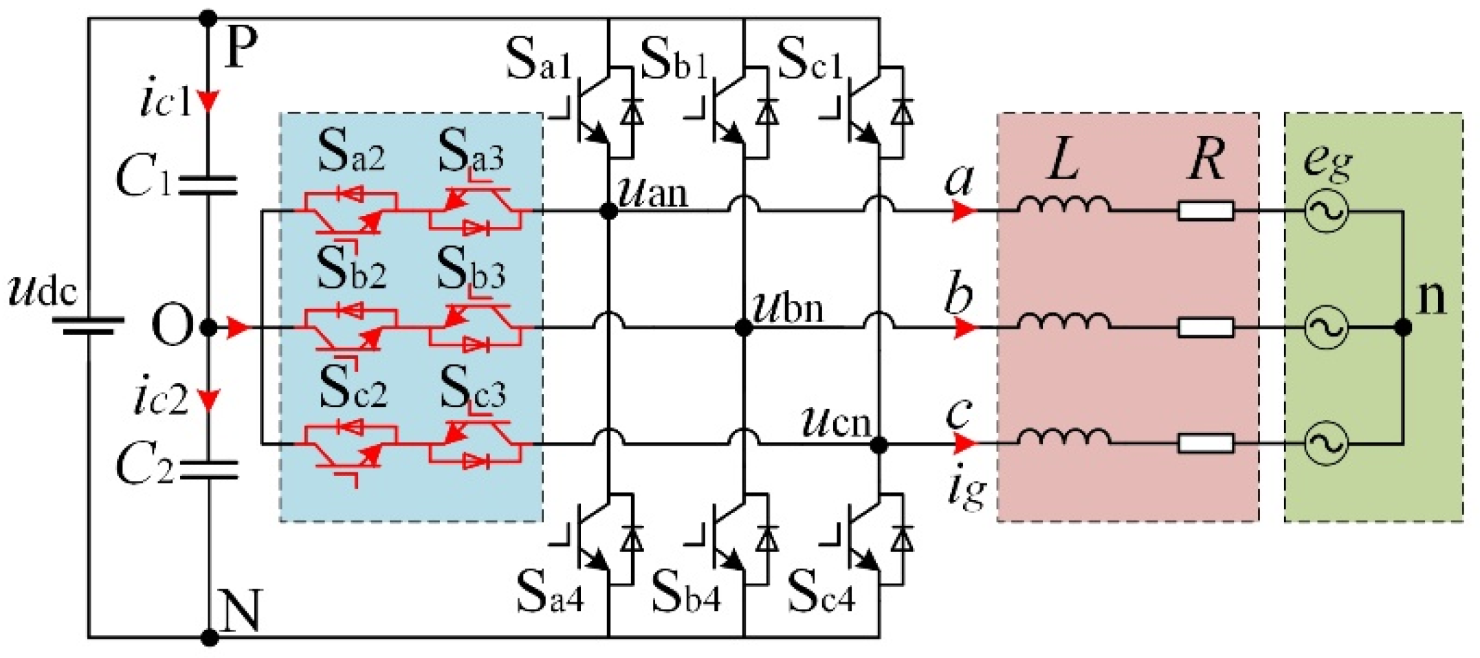
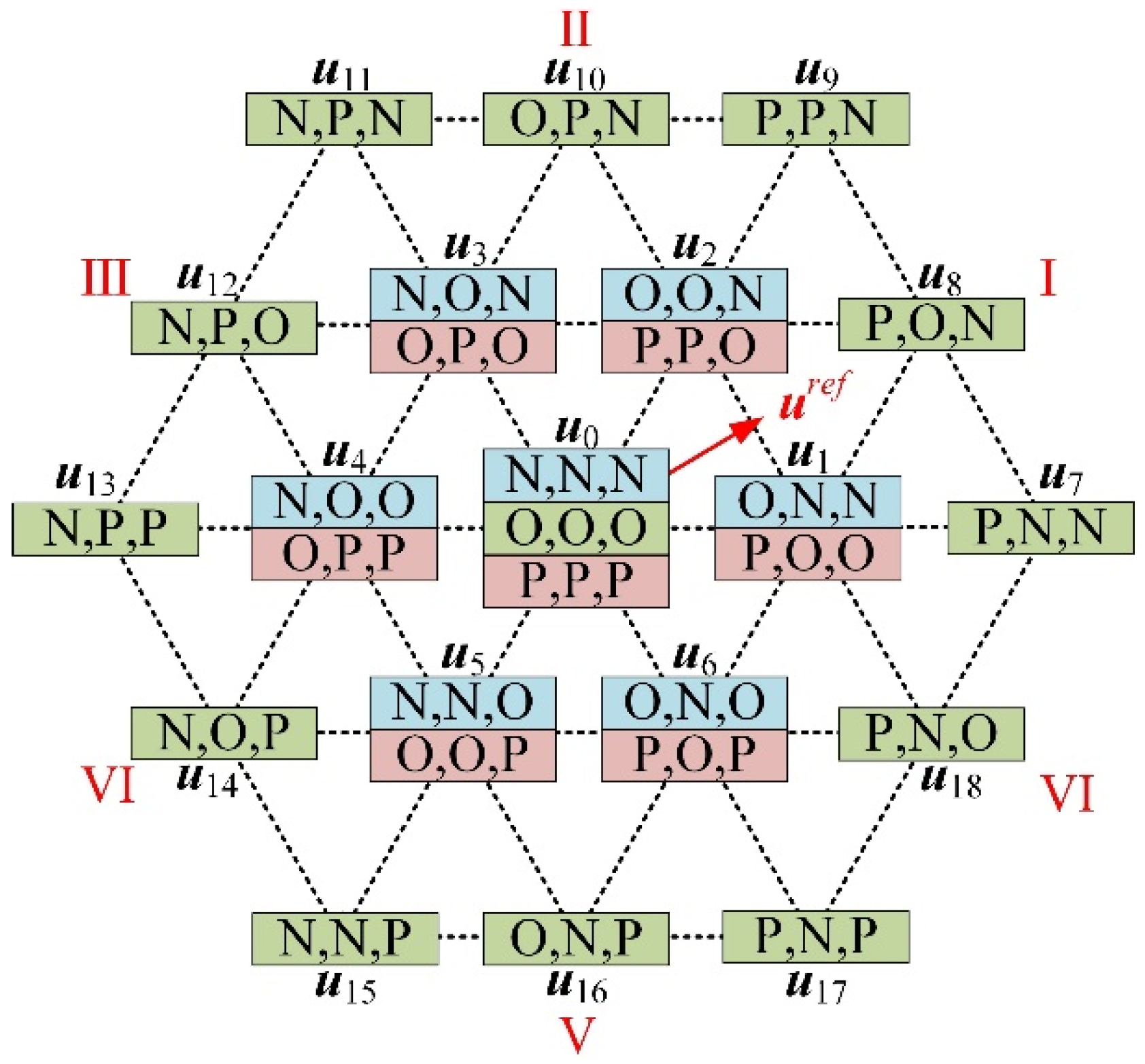
2.1. Topology and Voltage Vectors

The topology of the T-type three-level grid-tied inverter studied in this paper is shown in Figure 1, where u_dc is the dc-link voltage, and C₁ and C₂ are the upper and lower dc-link capacitors, respectively. O is the neutral point of dc-link capacitors and the zero-potential reference point. i_C1 and i_C2 are the current of C₁ and C₂, respectively. i_g is the output current. It can be seen from Figure 1 that each T-type three-level inverter bridge arm contains four switching tubes, which are S₁~S₄. There are three switching modes, including P, O, and N modes, based on the different switching combinations. All bridge arms share the neutral point of dc-link capacitors.

There are 27 voltage vectors that can be generated by a three-phase three-level inverter, as shown in Figure 2. The specific positions in Figure 2 corresponding to multiple space vectors are called redundant vectors, whose output characteristics are equivalent. According to the amplitude of the voltage vector, the 27 switching states can be divided into a zero vector (PPP, OOO, NNN), small vector (POO, PPO, OPO, OPP, OOP, ONN, OON, NON, NOO, NNO, ONO), medium vector (PON, OPN, NPO, NOP, ONP, PNO), and large vector (PNN, PPN, NPN, NPP, NNP, PNP).

2.2. Conventional Predictive Model

The principle of the conventional MPC scheme has been studied in many papers. Firstly, the mathematical model based on the LR-filtered three-level inverter connecting to grids in the α-β coordinate system can be expressed as

$$L\frac{d{i}_g}{dt}=u_x-R{i}_g-e_g$$

(1)

where u_x = [u_xα, u_xβ]^T, i_g = [i_gα, i_gβ]^T, and e_g = [e_gα, e_gβ]^T represent the output voltage vectors of the inverter, output current vectors, and grid voltage vectors, respectively. L represents the filter inductance and R represents the stray resistance.

The discrete model of the inverter can be expressed as

$$i_g^{}\left(k+1\right)=i_g\left(k\right)+\frac{T_s}{L}\left[u_x\left(k\right)-R{i}_g\left(k\right)-e_g\left(k\right)\right]$$

(2)

where T_s is the control period.

The voltage vector selected in the last control period can be used to calculate the prediction current i_g(k + 1) by (2). Then, all the voltage vectors shown in Figure 2 can be further used to calculate prediction currents i_gx(k + 2) by (3).

$$i_{gx}^{}\left(k+2\right)=\left(1-\frac{R{T}_s}{L}\right)i_g^{}\left(k+1\right)+\frac{T_s}{L}\left[u_x\left(k+1\right)-e_g\left(k+1\right)\right]$$

(3)

Finally, to evaluate the control performance of each voltage vector, a cost function shown in (4) is defined. The voltage vector that minimizes the cost function is used as the optimal vector and applied to the next control period.

$$G_x={\left(i_{ref}^{}(k+2)-i_{gx}^{}(k+2)\right)}^2$$

(4)

where i_ref(k + 2) are the reference currents.

In a three-level inverter control system, in addition to the output current, the neutral point voltage needs to be controlled. To avoid the design of weighting factor values when multiple control targets exist, MPC schemes without weighting factors have been proposed. In the MPC scheme without weighting factors, the P-type small vectors (POO, PPO, OPO, OPP, OOP) are considered as candidate vectors when the capacitor voltage u_c1 ≥ u_c2, and the N-type small vectors (ONN, OON, NON, NOO, NNO, ONO) are considered as candidate vectors when the capacitor voltage u_c1 < u_c2. The control block diagram of MPC is shown in Figure 3.

However, the prediction currents are affected when model parameters are mismatched with the controller parameters. The prediction currents with parameter errors can be expressed as

$$i_{gerr}(k+1)=i_g(k)+\frac{T_s}{L+\mathrm{\Delta }L}\left[u_x(k)-(R+\mathrm{\Delta }R)i_g(k)-e_g(k)\right]$$

(5)

where ∆L represents the inductance error between its actual value and its controller value, and ∆R represents the resistance error between its actual value and its controller value. Hence, it is important to enhance the parameter robustness of predictive control.

3. The Proposed MFPC Scheme

To eliminate the dependence on model parameters, an improved MFPC scheme based on a novel current gradient updating method is proposed in this section, including the basic principle of MFPC, the current gradient updating stagnation effect analysis, the proposed current gradient updating method, the sector judgment method, and the implementation steps.

3.1. Basic Principle of MFPC

In the MFPC scheme, the mathematical model (1) can be rewritten as [17]

$$\begin{array}{l}\Delta i_x\left(k-1\right)=\frac{T_s}{L}\left(u_x\left(k-1\right)-e_g\left(k-1\right)-R{i}_g\left(k-1\right)\right)\\ \hspace{1em}\hspace{1em} \hspace{1em}\hspace{1em} =i_g\left(k\right)-i_g\left(k-1\right) \hspace{0.17em}\end{array}$$

(6)

where ∆i_x(k − 1) = [∆i_xα(k − 1), ∆i_xβ(k − 1)]^T are the current gradients of the applied voltage vector u_x(k − 1). Although the switching states of redundant vectors are different, their coordinate components are the same. The multiple current gradients corresponding to redundant vectors are considered to be consistent. For example, voltage vector u₁ corresponds to two switching states of ONN and POO, so the current gradient corresponding to the two states is uniformly defined as ∆i₁. Hence, nineteen current gradients ∆i_x are stored in the look-up table (LUT) for current predictions, as shown in

Table 1. The LUT of the T-type three-level inverter.

Voltage Vector

u0

u1

u2

u3

u4

u5

u6

u7

u8

u9

u10

u11

u12

u13

u14

u15

u16

u17

u18

Current Gradient

∆i0

∆i1

∆i2

∆i3

∆i4

∆i5

∆i6

∆i7

∆i8

∆i9

∆i10

∆i11

∆i12

∆i13

∆i14

∆i15

∆i16

∆i17

∆i18

.

Then, the prediction currents at the (k + 1)th instant and the (k + 2)th instant can be calculated based on (7) and (8), respectively.

$$i_{gx}^{}\left(k+1\right)=i_g\left(k\right)+\Delta i_x\left(k\right)$$

(7)

$$i_{gx}^{}\left(k+2\right)=i_{gx}^{}\left(k+1\right)+\Delta i_x(k+1)$$

(8)

Finally, the optimal voltage vector u_op selected by cost function (4) is applied in the next control period.

3.2. Current Gradient Updating Stagnation Effect Analysis

It is obvious that the current prediction of MFPC is based on the current gradients which directly affect the accuracy of current prediction and the result of optimal voltage vector selection. The current gradients of applied voltage vectors are calculated based on (6) in the conventional MFPC scheme [20], however, the updating of the remaining current gradients stagnates. When the MFPC scheme is used in a three-level inverter system, the stagnation effect can be more obvious with the increasing number of voltage vectors, which not only affects the current performance but also affects the control of the neutral point voltage.

To reduce the updating stagnation effect, various current gradient updating methods have been reported in [21,22,23,24,30]; however, the updating stagnation is still existing. Hence, it is necessary to design an updating method to totally eliminate the stagnation effect.

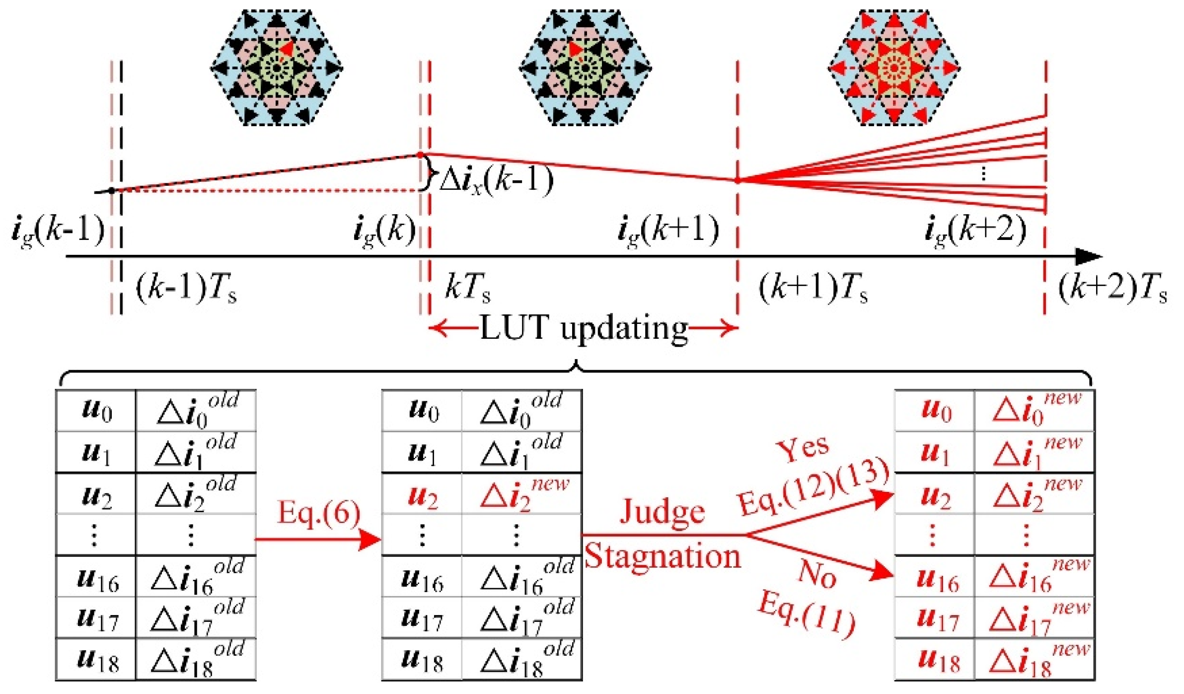
3.3. The Proposed Current Gradient Updating Method

In the proposed updating method, sampling points are set before switching states in each control period to avoid the current spikes. Based on (6), the relationship between the current gradient of remaining voltage vector ∆i_y and the current gradient of applied voltage vector ∆i_x at (k − 1)th instant and (k − 2)th instant can be expressed as (9) and (10), respectively.

$$\Delta i_y(k-1)-\Delta i_x(k-1)=\frac{T_s}{L}\left(u_y(k-1)-u_x(k-1)\right)$$

(9)

$$\Delta i_y(k-2)-\Delta i_x(k-2)=\frac{T_s}{L}\left(u_y(k-2)-u_x(k-2)\right)$$

(10)

The filter inductance L can be considered as a constant when T_s is short enough. Then, T_s/L of (9) and (10) can be eliminated by the division between (9) and (10), and the relationship between the current gradient in the two control periods can be written as

$$\Delta i_y(k-1)=\frac{u_y(k-1)-u_x(k-1)}{u_y(k-2)-u_x(k-2)}(\Delta i_y(k-2)-\Delta i_x(k-2))+\Delta i_x(k-1)$$

(11)

However, (11) cannot be used to update the current gradient when u_y(k − 2) − u_x(k − 2) = 0. In an α-axis coordinate system, seven situations may cause the stagnation effect. They are u_8α = u_18α, u_1α = u_9α = u_17α, u_2α = u_6α, u_0α = u_10α = u_16α, u_3α = u_5α, u_4α = u_11α = u_15α, and u_12α = u_14α, respectively. In a β-axis coordinate system, five situations may cause the stagnation effect. They are u_9β = u_10β = u_11β, u_2β = u_3β = u_8β = u_12β, u_0β = u_1β = u_4β = u_7β = u_13β, u_5β = u_6β = u_14β = u_18β, and u_15β = u_16β = u_17β, respectively. To eliminate the stagnation effect, (9) under the α-axis and β-axis is derived as (12) and (13), respectively. For example, when the applied voltage vector is u₂, ∆i_2αβ can be obtained based on (6). Then, in addition to ∆i_6α (calculated based on (12)), other α-axis current gradients can be calculated based on (11). Moreover, in addition to ∆i_3β, ∆i_8β, and ∆i_12β (calculated based on (13)), other β-axis current gradients can be calculated based on (11).

$$\Delta i_{y\alpha }(k-1)=\Delta i_{x\alpha }(k-1)$$

(12)

$$\Delta i_{y\beta }(k-1)=\Delta i_{x\beta }(k-1)$$

(13)

As a result, the stagnation effect is eliminated and the nineteen current gradients can be updated in each control period, as shown in Figure 4.

3.4. Proposed Sector Judgment Method

Conventionally, in order to find the optimal voltage vector through the cost function (4), 27 voltage vectors need to be traversed. When the redundancy state of the zero vector is ignored and the small vectors are selected as P-type small vectors or N-type small vectors according to the dc-link capacitor voltage difference, there are still 19 voltage vectors to be traversed. Since the calculation of reference voltage depends on the mathematical model, the sector judgment method based on reference voltage may cause sector judgment deviation when the model parameters are mismatched. Therefore, a sector judgment method based on the current gradient is proposed in this section.

Figure 5 shows the 19 voltage vectors and their corresponding 19 current gradients. The three-level inverter space vector coordinate system is divided into 6 large sectors and 24 small sectors. The position of the large sector where the reference current is located is judged according to the prediction currents of the medium vectors. For example, if the reference current is in large sector Ⅰ, the cost of u₈ calculated by (4) is the smallest compared with the cost of u₁₀, u₁₂, u₁₄, u₁₆, and u₁₈.

After judging the large sector, it is necessary to judge the small sector. First, the prediction currents can be calculated by (8). Then, the weighted error square ε² of the four small sectors can be calculated by (14) and selecting the smallest ε² corresponding sector as the target sector. Finally, there are only three voltage vectors as candidate vectors.

$${\epsilon }^2={\displaystyle \sum _{x=1}^3{\left(i_{ref}^{}(k+2)-i_{gx}^{}(k+2)\right)}^2}$$

(14)

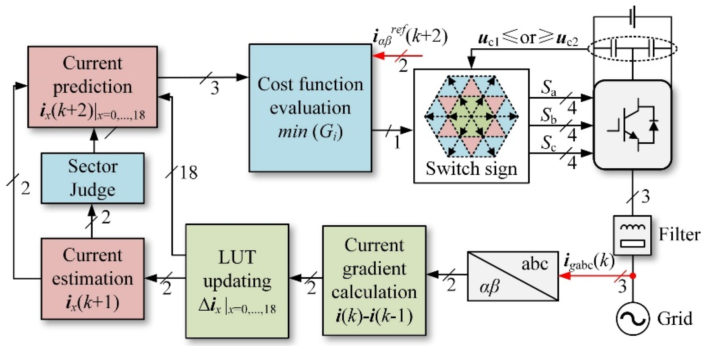
3.5. Implementation Steps

Figure 6 shows the control diagram of the proposed MFPC scheme. The proposed MFPC scheme is realized to eliminate parameter dependence, the novel current gradient updating method is realized to eliminate the stagnation effect, and the sector judgment method is also realized to further reduce the computational burden over the conventional MFPC scheme. The detailed implementation steps are as follows.

• Step I: Sample the dc-link capacitor voltage u_c1(k) and u_c2(k), select P-type basic voltage vectors or N-type basic voltage vectors based on u_c1(k) − u_c2(k) ≤ or >0.
• Step II: Sample the output current i_g(k) and calculate current gradient ∆i_x(k − 1) by (6).
• Step III: Update the remaining current gradients without stagnation effect by (11), and update the remaining current gradients with stagnation effect by (12) and (13).
• Step IV: Calculate prediction current i_gx(k + 1) and i_gx(k + 2) by (7) and (8), respectively.
• Step V: Judge large sectors by (4), and judge small sectors by (14).
• Step VI: Evaluate the cost of the three voltage vectors by (4) and select the optimal vector.

4. Simulation and Experimental Evaluation

In order to verify the effectiveness of the proposed MFPC scheme, simulations in MATLAB/Simulink and experiments under the conventional MPC scheme, conventional MFPC schemes, and the proposed MFPC scheme are carried out. Figure 7 depicts the T-type three-level three-phase grid-connected inverter experimental setup. The main control chip of the inverter is DSP28335. The sampling frequency is set as 20 kHz. The inverter parameters are listed in

Table 2. System and control parameters.

Parameters	Symbol	Values
DC-link voltage	udc	300 V
Peak of grid phase voltage	e	150 V
Grid angular frequency	ωg	314.16 rad/s
Control time	Ts	50 μs
Parasitic resistance	R	0.05 Ω
Filter inductance	L0	10 mH

.

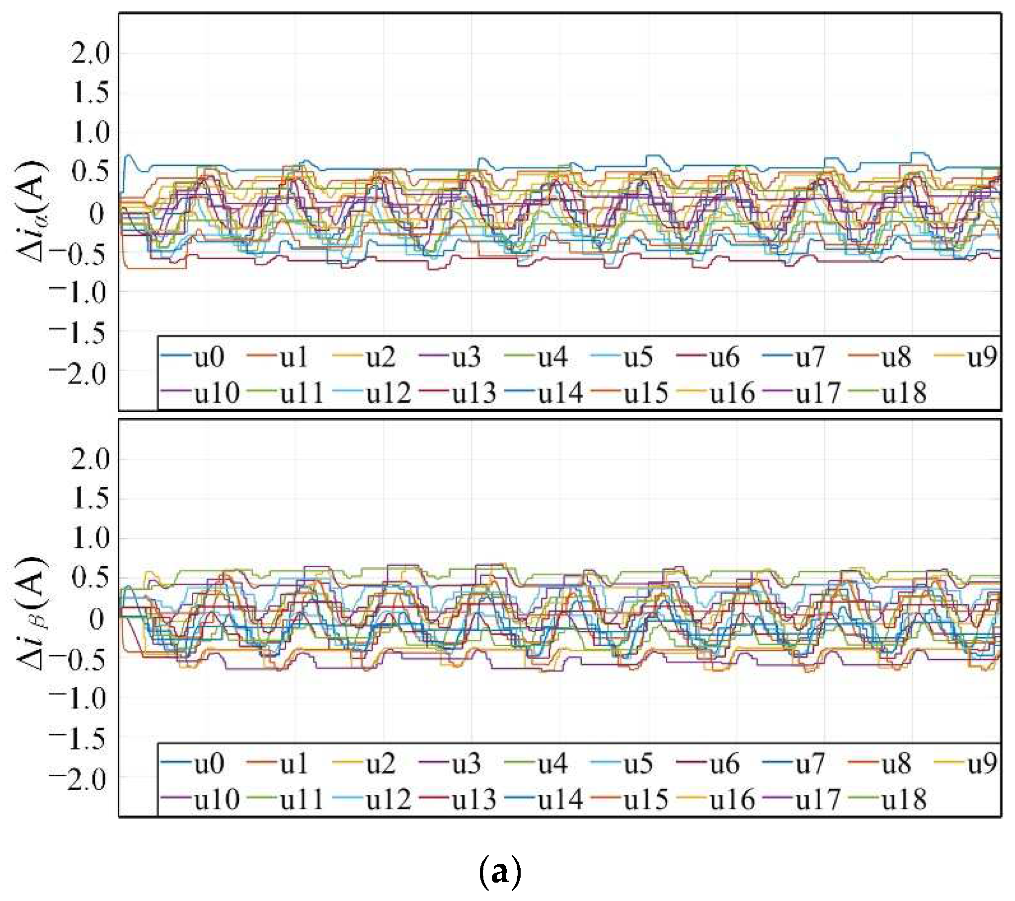
4.1. Impact of Current Gradient Updating Stagnation

The proposed current gradient updating method is compared with the updating method in [20] and the updating method in [30]. Figure 8a illustrates the α-axis and β-axis current gradients when the updating method in [20] is used. In this current gradient updating method, there is a notable stagnation effect in both the current gradients ∆i_α and ∆i_β because the current gradients of the applied voltage vector can be updated for the LUT; however, the remaining current gradients keep the old values. Compared to the two-level inverter system [20], the stagnation effect becomes more obvious with the increasing number of voltage vectors when the updating method [20] is used in the three-level inverter system. As shown in Figure 8b, although the updating frequency is improved, the stagnation effect still exists in the α-axis and β-axis current gradients when the updating method in [30] is used. When the updating method is converted to the proposed updating method, it can be seen that there is no stagnation effect existing in the current gradient waveforms, as shown in Figure 8b, which shows the effectiveness of the proposed updating method.

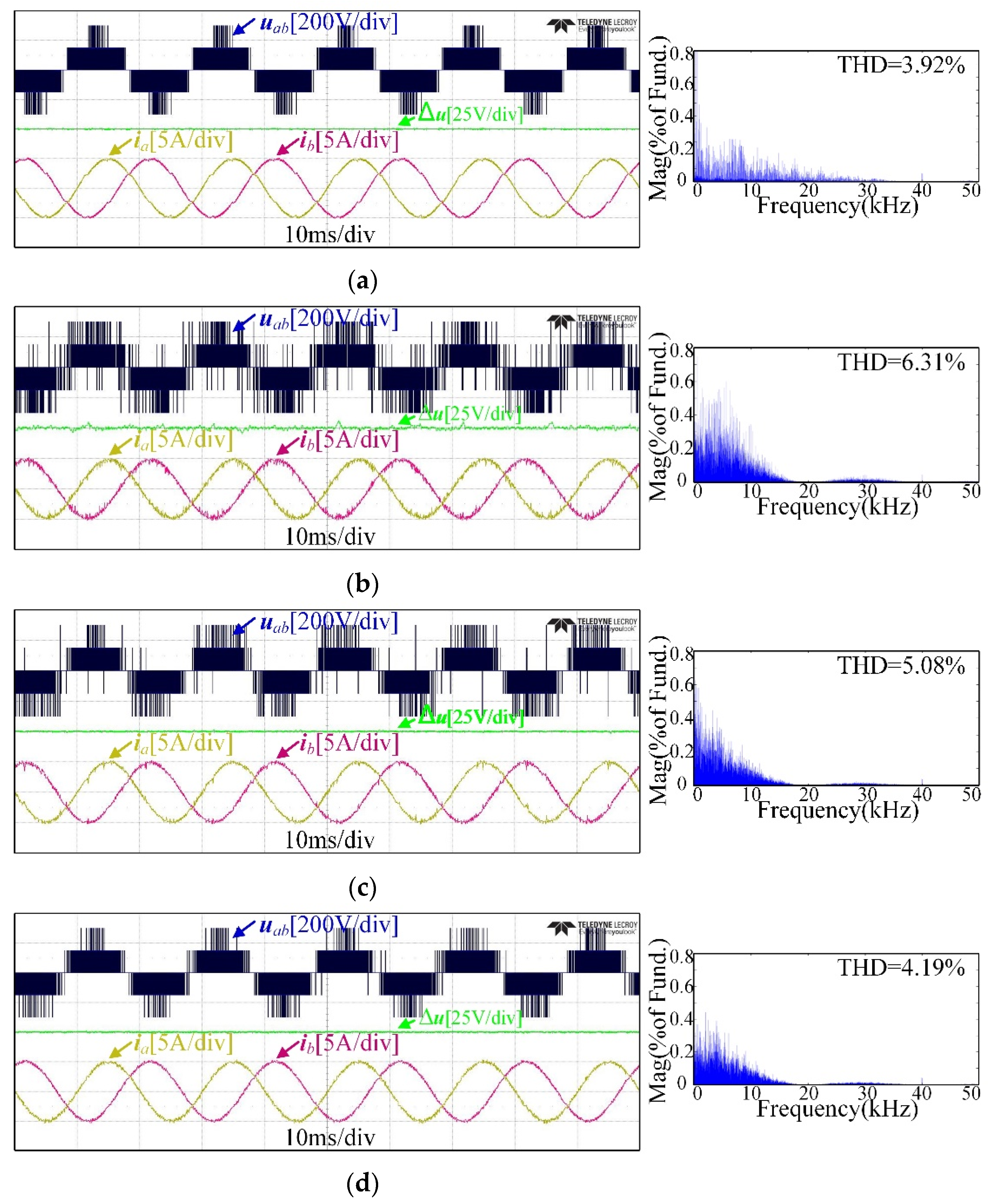
4.2. Steady-State Experimental Evaluation

Figure 9 shows the steady-state performance comparisons of the conventional MPC scheme, conventional MFPC scheme in [20], conventional MFPC scheme in [30], and the proposed MFPC scheme when model parameters match controller parameters. Based on the steady-state experimental waveforms, it can be seen that both the conventional MPC scheme, the conventional MFPC scheme in [30], and the proposed MFPC scheme can achieve tracking the reference currents and balancing the neutral point voltages. However, the neutral point voltage of the conventional MFPC scheme in [20] is affected by the current gradient stagnation effect. The harmonic spectra of the current are drawn by MATLAB/Simulink with the experimental data obtained from the oscilloscope, as shown in Figure 9.

For the conventional MPC scheme, the total harmonic distortion (THD) of phase-a output current is 3.92%. For the conventional MFPC scheme in [20], the THD of phase-a output current changes from 3.92% to 6.31% because the current performance is affected by the stagnation effect and the sampling noise effect. For the conventional MFPC scheme in [30], the THD of phase-a output current changes from 6.31% to 5.08% because the stagnation effect is improved, but it cannot be eliminated. Moreover, the current spikes caused by the stagnation effect can be observed simultaneously in Figure 9b,c. Compared with the conventional MFPC scheme in [30], the THD of phase-a output current reduces from 5.08% to 4.19% because the stagnation effect is eliminated, as shown in Figure 9d. However, the current performance of the proposed scheme is worse than that of the conventional MPC scheme because the current performance of the MFPC scheme is affected by the sampling noise.

To further verify the effectiveness of the proposed MFPC scheme, other experimental comparisons under different reference currents are carried out. The THDs of phase-a current under four control schemes are shown in Figure 10. From Figure 10, the THDs of the four control schemes are reduced with the increased reference currents. The proposed MFPC still has a similar current THD to the MPC and has a lower current THD than the MFPC in [20] and the MFPC in [30].

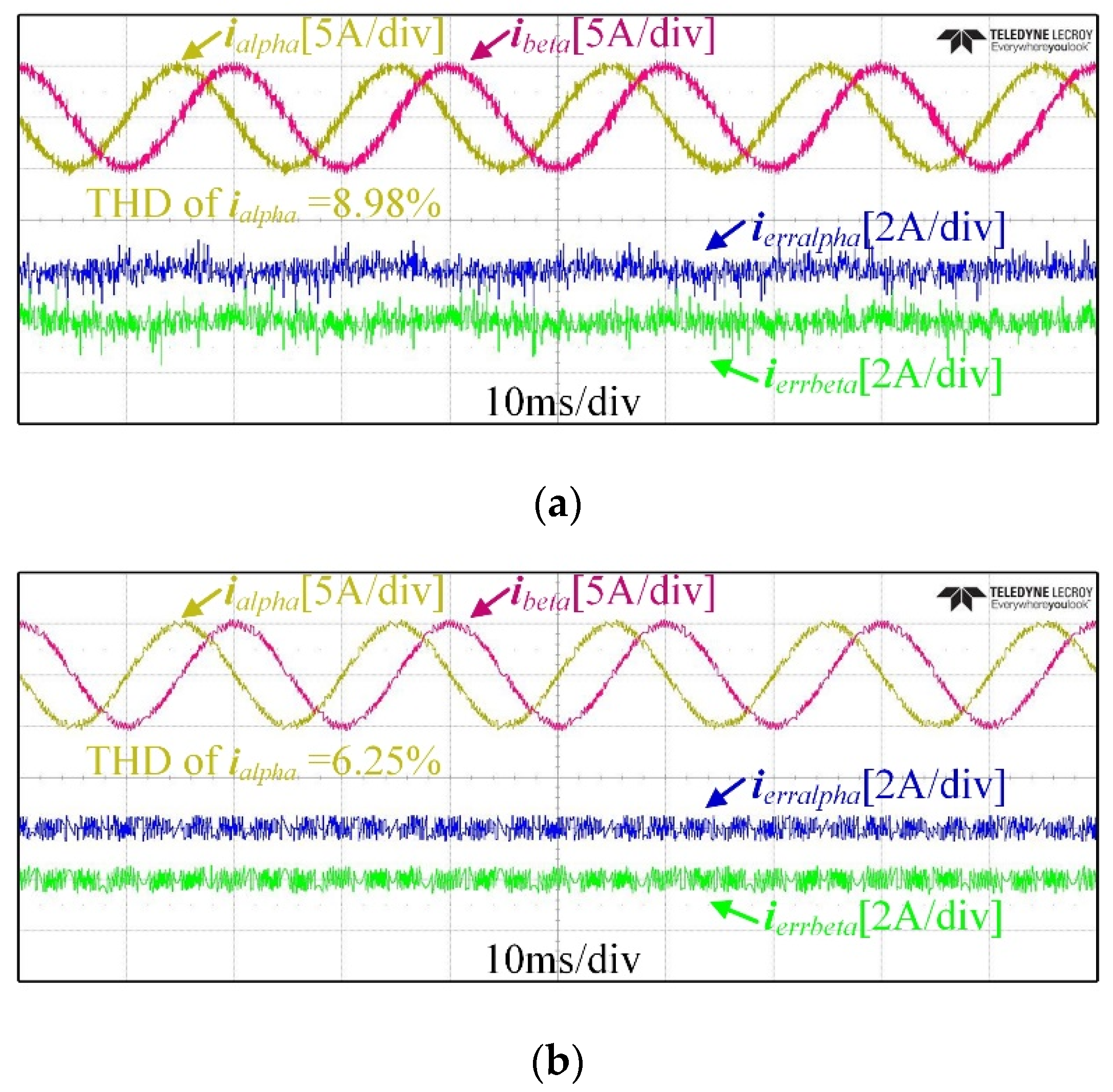
4.3. Experimental Evaluation under Mismatched Model Parameters

To verify the effectiveness of the proposed MFPC scheme in enhancing parameter robustness, the control performance of the proposed scheme and the conventional MPC scheme are compared in this section when the filter inductance as the model parameter is taken as different actual values from the controller values L₀. It can be seen that compared with the conventional MPC scheme, the proposed scheme reduces the THD from 8.98% to 6.25% when the actual filter inductance is set as 0.05 H (i.e., 0.5L₀) as shown in Figure 11. Additionally, the proposed scheme reduces the THD from 2.78% to 1.87% when the actual filter inductance is set as 0.2 H (i.e., 2L₀), as shown in Figure 12. Under the above two experimental conditions, the current prediction errors of the proposed scheme are lower than that of the conventional MPC scheme. The current waveforms, the THDs, and the current prediction errors verify that the proposed scheme has stronger parameter robustness than the conventional MPC scheme.

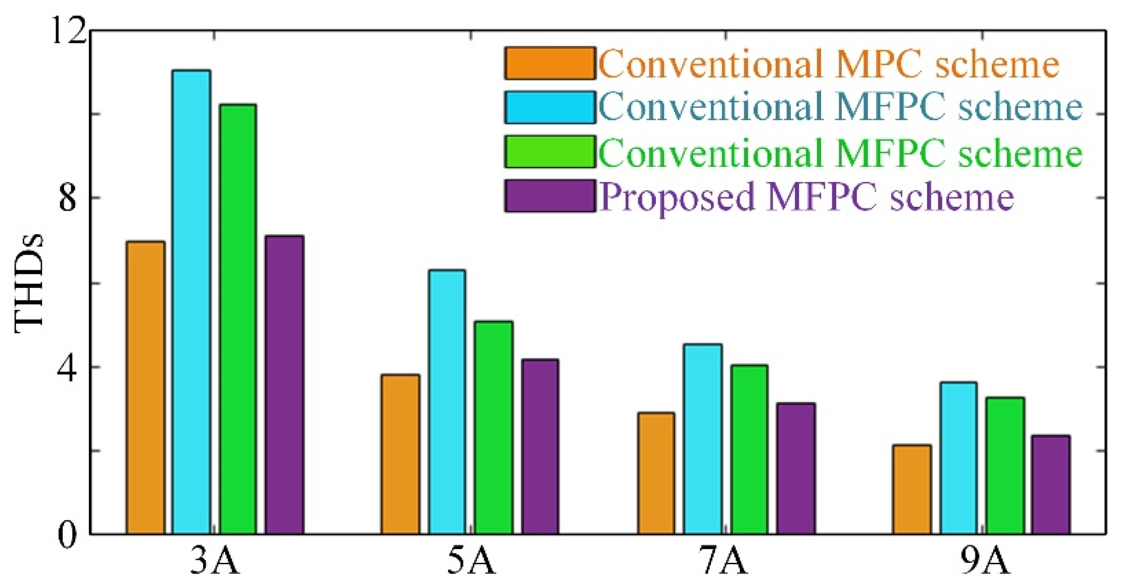
4.4. Performance Comparison of All Schemes

In order to further demonstrate the advantages of the proposed MFPC, various performances of all schemes are compared and summarized in

Table 3. Performance comparison of different control schemes.

Schemes	THDs	Computational Burden	Parameter Robustness	Stagnation Elimination
Conventional MPC	3.92%	35.9 μs	No	-
Conventional MFPC in [20]	6.31%	31.8 μs	Yes	No
Conventional MFPC in [30]	5.08%	41.2 μs	Yes	No
Proposed MFPC	4.19%	36.2 μs	Yes	Yes

, including THDs, computational burden, parameter robustness, and stagnation effect. The proposed MFPC has a similar THD to MPC when model parameters are accurate and have better robustness against mismatched parameters than MPC. Though 18 current gradients in the proposed MFPC should be updated per control period, the speed of optimization is effectively reduced by the proposed sector judgment method. Hence, the proposed MFPC has a similar computational burden to MPC. For the MFPC in [20,30], although they cannot be affected by the mismatched parameters, their THDs are higher than those of the proposed MFPC because of the stagnation effect. For the MFPC in [20], it has the smallest computational burden because there is no current gradient updating exists, which leads to the largest THD. For MFPC in [30], it has the largest computational burden because there is all current gradient is updated and candidate voltage vectors are not reduced.

5. Conclusions

This paper proposes an improved MFPC scheme based on the novel current gradient updating method and the effective sector judgment method for a T-type three-level grid-tied inverter. The proposed scheme has the following salient features: First, compared to conventional MPC schemes without a weighting factor, it totally eliminates the effect of mismatched model parameters and enhances the parameter robustness, especially when the actual parameters are less than the control parameters. Then, compared to conventional MPC schemes using a weighting factor, it avoids designing the weight factor and still realizes the good control of current and neutral point voltage. Moreover, compared to conventional MFPC schemes, it eliminates the current gradient stagnation effect by the designed updating method. The THDs of the proposed scheme decrease by up to 2.12% and the current spikes caused by the long updating stagnation are avoided. Finally, the discrimination accuracy of redundant small vectors is improved by using the proposed sector judgment method based on the current gradient, and the speed of optimization is increased by 31.5%.

References

1. Zhang, Z.; Xu, H.; Xue, M.; Chen, Z.; Sun, T.; Kennel, R.; Hackl, C.M. Predictive control with novel virtual-flux estimation for back-to-back power converters. IEEE Trans. Ind. Electron. 2015, 62, 2823–2834. [Google Scholar] [CrossRef]
2. Zhao, T.; Chen, D. A power adaptive control strategy for further extending the operation range of single-phase cascaded H-bridge multilevel PV inverter. IEEE Trans. Ind. Electron. 2022, 69, 1509–1520. [Google Scholar] [CrossRef]
3. Adefarati, T.; Bansal, R.C. Integration of renewable distributed generators into the distribution system: A review. IET Renew. Power Gener. 2016, 10, 873–884. [Google Scholar] [CrossRef]
4. Freddy, T.K.S.; Rahim, N.A.; Hew, W.P.; Che, H.S. Comparison and analysis of single-phase transformerless grid-connected PV inverters. IEEE Trans. Power Electron. 2014, 29, 5358–5369. [Google Scholar] [CrossRef]
5. Schweizer, M.; Kolar, J.W. Design and implementation of a highly efficient three-level t-type converter for low-voltage application. IEEE Trans. Power Electron. 2013, 28, 1504–1511. [Google Scholar] [CrossRef]
6. Schweizer, M.; Lizama, I.; Friedli, T.; Kolar, J.W. Comparison of the chip area usage of 2-level and 3-level voltage source converter topologies. In Proceedings of the IECON 2010-36th Annual Conference on IEEE Industrial Electronics Society, Glendale, AZ, USA, 7–10 November 2010; pp. 391–396. [Google Scholar]
7. Karamanakos, P.; Geyer, T. Model Predictive Torque and Flux Control Minimizing Current Distortions. IEEE Trans. Power Electron. 2019, 34, 2007–2012. [Google Scholar] [CrossRef]
8. Yan, L.; Wang, F.; Dou, M.; Zhang, Z.; Kennel, R.; Rodríguez, J. Active Disturbance-Rejection-Based Speed Control in Model Predictive Control for Induction Machines. IEEE Trans. Ind. Electron. 2020, 67, 2574–2584. [Google Scholar] [CrossRef]
9. Guo, L.; Jin, N.; Gan, C.; Luo, K. Hybrid Voltage Vector Preselection-Based Model Predictive Control for Two-Level Voltage Source Inverters to Reduce the Common-Mode Voltage. IEEE Trans. Ind. Electron. 2020, 67, 4680–4691. [Google Scholar] [CrossRef]
10. Young, H.A.; Perez, M.A.; Rodriguez, J. Analysis of Finite-Control-Set Model Predictive Current Control with Model Parameter Mismatch in a Three-Phase Inverter. IEEE Trans. Ind. Electron. 2016, 63, 3100–3107. [Google Scholar] [CrossRef]
11. Zhang, X.; Zhang, L.; Zhang, Y. Model Predictive Current Control for PMSM Drives with Parameter Robustness Improvement. IEEE Trans. Power Electron. 2019, 34, 1645–1657. [Google Scholar] [CrossRef]
12. Zhang, Y.; Li, B.; Liu, J. Online Inductance Identification of a PWM Rectifier under Unbalanced and Distorted Grid Voltages. IEEE Trans. Ind. Appl. 2020, 56, 3879–3888. [Google Scholar] [CrossRef]
13. Niu, S.; Luo, Y.; Fu, W.; Zhang, X. Robust Model Predictive Control for a Three-Phase PMSM Motor with Improved Control Precision. IEEE Trans. Ind. Electron. 2021, 68, 838–849. [Google Scholar] [CrossRef]
14. Yan, L.; Dou, M.; Hua, Z. Disturbance Compensation-Based Model Predictive Flux Control of SPMSM with Optimal Duty Cycle. IEEE J. Emerg. Sel. Top. Power Electron. 2019, 7, 1872–1882. [Google Scholar] [CrossRef]
15. Wang, J.; Wang, F.; Wang, G.; Li, S.; Yu, L. Generalized Proportional Integral Observer Based Robust Finite Control Set Predictive Current Control for Induction Motor Systems with Time-Varying Disturbances. IEEE Trans. Ind. Inf. 2018, 14, 4159–4168. [Google Scholar] [CrossRef]
16. Zoghdar-Moghadam-Shahrekohne, B.; Pozzi, A.; Raimondo, D.M. SOS-based Stability Region Enlargement of Bilinear Power Converters through Model Predictive Control. In Proceedings of the 2021 29th Mediterranean Conference on Control and Automation (MED), Bari, Italy, 22–25 June 2021; pp. 847–854. [Google Scholar]
17. Zhang, Y.; Jiang, T.; Jiao, J. Model-Free Predictive Current Control of a DFIG Using an Ultra-Local Model for Grid Synchronization and Power Regulation. IEEE Tran. Energy Convers. 2020, 35, 2269–2280. [Google Scholar] [CrossRef]
18. Jin, N.; Chen, M.; Guo, L.; Li, Y.; Chen, Y. Double-Vector Model-Free Predictive Control Method for Voltage Source Inverter With Visualization Analysis. IEEE Trans. Ind. Electron. 2022, 69, 10066–10078. [Google Scholar] [CrossRef]
19. Rodríguez, J.; Heydari, R.; Rafiee, Z.; Young, H.A.; Flores-Bahamonde, F.; Shahparasti, M. Model-Free Predictive Current Control of a Voltage Source Inverter. IEEE Access 2020, 8, 211104–211114. [Google Scholar] [CrossRef]
20. Lin, C.; Liu, T.; Yu, J.; Fu, L.; Hsiao, C. Model-Free Predictive Current Control for Interior Permanent-Magnet Synchronous Motor Drives Based on Current Difference Detection Technique. IEEE Trans. Ind. Electron. 2014, 61, 667–681. [Google Scholar] [CrossRef]
21. Lin, C.; Yu, J.; Lai, Y.; Yu, H. Improved Model-Free Predictive Current Control for Synchronous Reluctance Motor Drives. IEEE Trans. Ind. Electron. 2016, 63, 3942–3953. [Google Scholar] [CrossRef]
22. da Rù, D.; Polato, M.; Bolognani, S. Model-free predictive current control for a SynRM drive based on an effective update of measured current responses. In Proceedings of the 2017 IEEE International Symposium on Predictive Control of Electrical Drives and Power Electronics (PRECEDE), Pilsen, Czech Republic, 4–6 September 2017; pp. 119–124. [Google Scholar]
23. Carlet, P.G.; Tinazzi, F.; Bolognani, S.; Zigliotto, M. An Effective Model-Free Predictive Current Control for Synchronous Reluctance Motor Drives. IEEE Trans. Ind. Appl. 2019, 55, 3781–3790. [Google Scholar] [CrossRef] [Green Version]
24. Ma, C.; Li, H.; Yao, X.; Zhang, Z.; de Belie, F. An Improved Model-Free Predictive Current Control with Advanced Current Gradient Updating Mechanism. IEEE Trans. Ind. Electron. 2021, 68, 11968–11979. [Google Scholar] [CrossRef]
25. Agustin, C.A.; Yu, J.-T.; Lin, C.-K.; Jai, J.; Lai, Y.-S. Triple-Voltage-Vector Model-Free Predictive Current Control for Four-Switch Three-Phase Inverter-Fed SPMSM Based on Discrete-Space-Vector Modulation. IEEE Access 2021, 9, 60352–60363. [Google Scholar] [CrossRef]
26. Agustin, C.A.; Yu, J.-T.; Cheng, Y.-S.; Lin, C.-K.; Huang, H.-Q.; Lai, Y.-S. Model-Free Predictive Current Control for SynRM Drives Based on Optimized Modulation of Triple-Voltage-Vector. IEEE Access 2021, 9, 130472–130483. [Google Scholar] [CrossRef]
27. Lin, C.-K.; Yu, J.-T.; Agustin, C.A.; Li, N.-Y. A Two-Staged Optimization Approach to Modulated Model-Free Predictive Current Control for RL-Connected Three-Phase Two-Level Four-Leg Inverters. IEEE Access 2021, 9, 147537–147548. [Google Scholar] [CrossRef]
28. Lin, C.-K.; Agustin, C.A.; Yu, J.-T.; Cheng, Y.-S.; Chen, F.-M.; Lai, Y.-S. A Modulated Model-Free Predictive Current Control for Four-Switch Three-Phase Inverter-Fed SynRM Drive Systems. IEEE Access 2021, 9, 162984–162995. [Google Scholar] [CrossRef]
29. Agustin, C.A.; Yu, J.-T.; Cheng, Y.-S.; Lin, C.-K.; Yi, Y.-W. A Synchronized Current Difference Updating Technique for Model-Free Predictive Current Control of PMSM Drives. IEEE Access 2021, 9, 63306–63318. [Google Scholar] [CrossRef]
30. Yu, F.; Zhou, C.; Liu, X.; Zhu, C. Model-Free Predictive Current Control for Three-Level Inverter-Fed IPMSM With an Improved Current Difference Updating Technique. IEEE Trans. Energy Convers. 2021, 36, 3334–3343. [Google Scholar] [CrossRef]
31. Ipoum-Ngome, P.G.; Mon-Nzongo, D.L.; Flesch, R.C.C.; Song-Manguelle, J.; Wang, M.; Jin, T. Model-Free Predictive Current Control for Multilevel Voltage Source Inverters. IEEE Trans. Ind. Electron. 2021, 68, 9984–9997. [Google Scholar] [CrossRef]
Figure 1. Topology of the T-type three-level grid-tied inverter.
Energies 15 06557 g001
Figure 2. Basic voltage vectors of the three-level three-phase inverter.
Energies 15 06557 g002
Figure 3. Control block diagram of the conventional MPC scheme.
Energies 15 06557 g003
Figure 4. Proposed current gradient updating method.
Energies 15 06557 g004
Figure 5. Big and small sectors of the three-level three-phase inverter.
Energies 15 06557 g005
Figure 6. Control block diagram of the proposed MFPC scheme.
Energies 15 06557 g006
Figure 7. T-type three-level three-phase grid-connected inverter experimental platform.
Energies 15 06557 g007
Figure 8. Current gradient comparisons under different updating methods (iref = 5A). (a) Updating method in [20]. (b) Updating method in [30]. (c) The proposed updating method.
Energies 15 06557 g008aEnergies 15 06557 g008b
Figure 9. Experimental waveform comparisons (iref = 5A). (a) Waveforms under the conventional MPC scheme. (b) Waveforms under the conventional MFPC scheme in [20]. (c) Waveforms under the conventional MFPC scheme in [30]. (d) Waveforms under the proposed MFPC scheme.
Energies 15 06557 g009
Figure 10. The comparison of phase-a current THDs under different reference currents.
Energies 15 06557 g010
Figure 11. Experimental waveforms comparisons when L/L0 = 0.5 (iref = 5A). (a) Waveforms under the conventional MPC scheme. (b) Waveforms under the proposed MFPC scheme.
Energies 15 06557 g011
Figure 12. Experimental waveforms comparisons when L/L0 = 2 (iref = 5A). (a) Waveforms under the conventional MPC scheme. (b) Waveforms under the proposed MFPC scheme.
Energies 15 06557 g012