Small-Signal Stability Research of Grid-Connected Virtual Synchronous Generators

Abstract

The virtual synchronous generator (VSG) technique is used to simulate the external characteristics of a synchronous generator (SG) to provide certain damping and inertia to power systems. However, it may easily cause low-frequency oscillation of the power system. We studied the small-signal stability of a grid-connected virtual synchronous generator. Firstly, the small-signal models of single-VSG and multi-VSG grid-connected systems were established. Subsequently, the system eigenvalues were obtained by solving the state matrix, and the system oscillation modes were analyzed. The eigenvalue analysis method was used to analyze the impacts of parameter changes, such as virtual moment of inertia, virtual damping coefficient, line resistance, and line inductance, on system stability. Finally, our conclusions were verified by numerous simulation models.

1. Introduction

Many new energy units are connected to the power system through inverters, and the proportion of power electronic devices in the power system has increased rapidly [1]. The operation mode and dynamic characteristics of the power grid have changed gradually [2,3,4]. A power system including fewer synchronous generators (SG) and more power electronic devices cannot provide sufficient physical damping and inertia, which is not conducive to the stable operation of the power system [5].

To solve the above problems, the virtual synchronous generator (VSG) technique is proposed [6,7]. The VSG considers the electromechanical and excitation transient characteristics of synchronous generators to provide virtual damping and inertia [8]. However, although VSG simulates the excellent regulation characteristics of SG, low-frequency oscillation problems will occur and the oscillation mode will be changed [9,10]. Therefore, the grid-connected stability of VSG needs to be further analyzed. In this regard, single-VSG and multi-VSG grid-connected stabilities are widely studied.

In the study of single-machine grid connection stability, Reference [11] developed a double-machine test-bed to analyze the low-frequency oscillation phenomenon after VSG replaces SG, as well as the characteristics and main modes of low-frequency oscillation, and evaluated the role of the power system stabilizer in the VSG grid. In [12], the internal voltage of the inverter was taken as a parameter rather than a state variable, and the voltage change was introduced into the approximate Lyapunov direct method. The influence of the reactive power voltage control link and different parameters on the stability of VSG was analyzed, and it was pointed out that the reactive power control loop will reduce the stability margin of the VSG power angle. Reference [13] proposed the concepts of virtual common coupling point and virtual power angle to represent the mathematical model of a variable cross-section vibration generator with virtual damping and analyzed the transient stability of VSG. In [14], a small-signal model of a VSG-SG interconnected system suitable for studying the low-frequency oscillation damping of the transmission network is proposed. Through this model, the influence of VSG and SG on the power system is compared, and the mechanism of VSG’s influence on damping characteristics is revealed. In [15], the VSG small-signal model of voltage and current double closed loop and active and reactive power control was established to study the VSG oscillation characteristics. The analysis showed that the reactive power loop and DQ axis voltage control have a great impact on the damping of low-frequency oscillation.

In the research on the stability of multi-machine parallel connection, in [16], the VSG-based active power frequency loop is equivalent to P/ω. The two-terminal-network model of “admittance” analyzes the three kinds of factors that affect the output power of VSG and the power frequency oscillation characteristics of the three kinds of factors when the parameters change. Reference [17] defines the deviation of generator voltage angle relative to inertia center angle as a tool to evaluate the stability of a multi-VSG microgrid and optimizes VSG unit parameters through the particle swarm optimization algorithm. Reference [18] studies a new method to improve the transient stability of a multi-VSG power grid, which suppresses the oscillation between VSG and the inertial frequency center of the power grid during short circuit. Reference [19] proposes a fully decentralized mutual damping method to solve the problem of power oscillation in parallel with multiple VSGs. By introducing the derivative of local power, the difference between each angular frequency is obtained indirectly, which effectively suppresses power oscillation. In [20], secondary frequency control of a distributed VSG for low-bandwidth communication is proposed, which suppresses oscillation and restores the frequency to the rated value without changing the virtual inertia provided by VSG.

To summarize, the theory of VSG grid connection stability is gradually maturing, but the extant literature does not discuss the specific impact of the changes in various parameters in VSG on the low-frequency oscillation mode of the power system after VSG grid connection, as well as the dominant factors in the change in oscillation mode. Moreover, nowadays, the stability research on VSG control mostly adopts the damping torque analysis method. Although this method is easy to build a complex global model, its stability criteria are complex and the parameter regions are difficult to identify [21]. The eigenvalue analysis method in the small-signal analysis method can better analyze the stability of the system when the parameters change. Therefore, we present here a more in-depth study on the grid connection stability of a virtual synchronous generator based on the small-signal model analysis method. The influence of VSG parameters on the stability of a single-machine grid-connected system and a multi-machine grid-connected system is analyzed through system eigenvalue trajectories. The main contributions are as follows:

(1) Based on the topology and algorithm of VSG, small-signal modeling is carried out for a single-machine grid-connected system and a multi-machine parallel grid-connected system.

(2) In the single-machine grid-connected system, the influences of oscillation mode, control parameters of active power loop, and resistance inductance ratio of connecting line on eigenvalues are analyzed.

(3) In the multi-machine parallel connected system, the effects of virtual moment of inertia, damping coefficient, line resistance, and line inductance on the eigenvalues are analyzed. Finally, the conclusions are verified by numerous simulation models.

2. VSG Control Strategy

2.1. VSG Topology

The topology of the virtual synchronous generator is shown in Figure 1. VSG can be divided into four layers. The first layer is the power loop controller, which is composed of an abc/dq transformation link and a power calculation module. The second layer is the VSG control algorithm, which is used to generate the voltage references. The third layer is the voltage and current double closed-loop controllers, which consist of voltage and current double closed-loop modules and dq/abc transformation. The fourth layer is sinusoidal pulse width modulation.

In Figure 1, u_dc is the ideal DC voltage on the DC side, R_f is resistance, L_f is inductance, and C_f is capacitance. R_c and L_c are the resistance and inductance of the connecting line. u_a, u_b, and u_c are the output voltage of the inverter. i_a, i_b, and i_c are the output currents of the inverter. i_oa, i_ob, and i_oc are the currents of the line inductance. u_oa, u_ob, and u_oc are the filter capacitor voltages. u_ga, u_gb, and u_gc are the AC power grid voltages. P_ref is the active power, and Q_ref is the reactive power.

2.2. VSG Algorithm

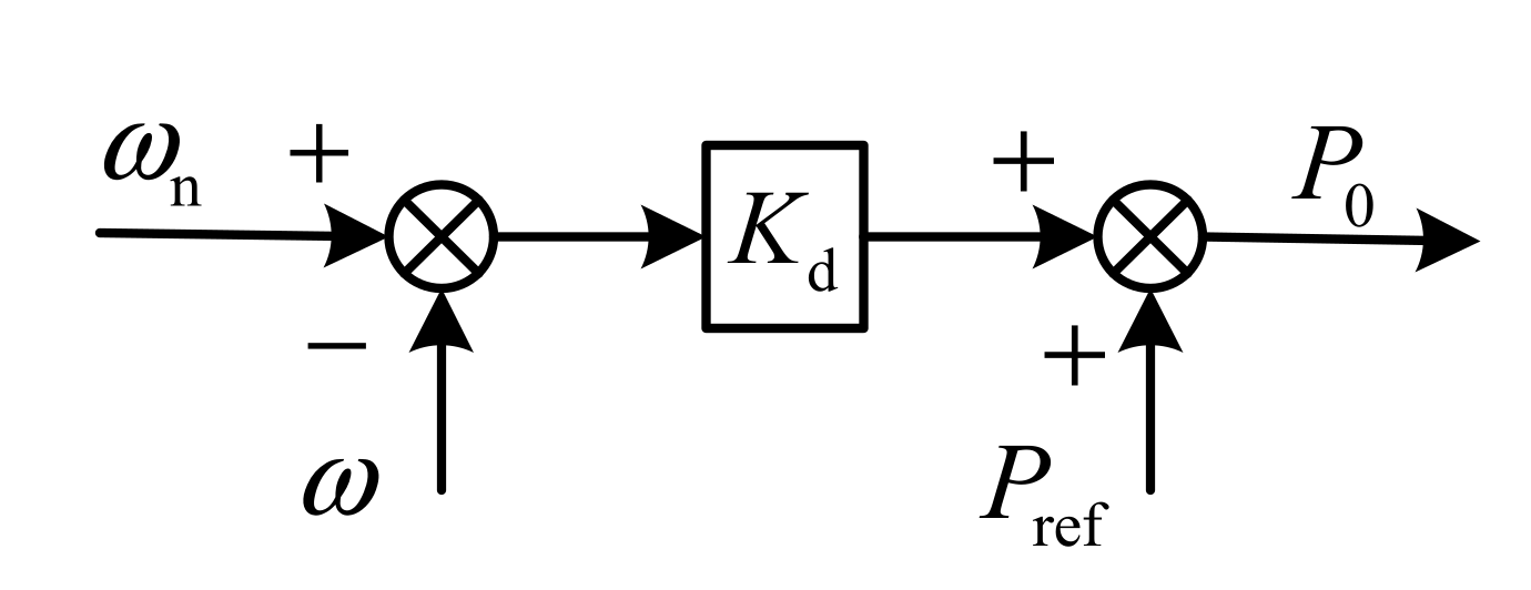
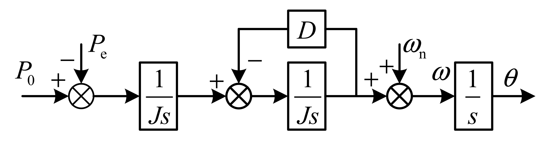
2.2.1. Virtual Power Frequency Controller

To realize the simulation of the synchronous generator governor, the virtual speed regulator in VSG usually adopts frequency droop control to realize primary frequency regulation, and its control structure is shown in Figure 2.

In Figure 2, ω_n is the rated angular frequency of VSG, ω is the output virtual angular frequency, K_d is the active frequency regulation coefficient of the governor, and P₀ is the mechanical power.

As we know, the inertia and damping characteristics are mainly controlled by the mechanical rotational inertia of the rotor, which are transient regulation characteristics. The adequate damping can suppress overshoot and oscillations of output. The virtual moment of inertia control in VSG is shown in Figure 3.

In Figure 3, J is the VSG virtual moment of inertia, D is the VSG virtual damping coefficient, P_e is the electromagnetic power, and θ is the electrical angle.

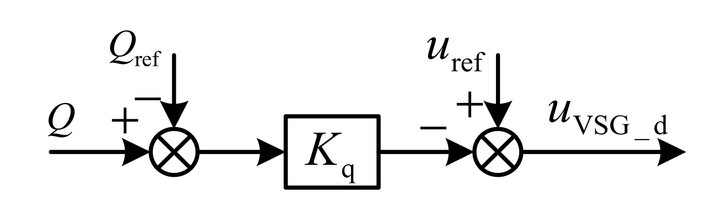
2.2.2. Virtual Excitation Controller

The virtual excitation regulator in VSG adopts reactive voltage droop control to realize the voltage regulation characteristics of the excitation system of SG. The block diagram of VSG virtual excitation control is shown in Figure 4.

In Figure 4, K_q is the reactive voltage regulation coefficient of the excitation controller, and u_ref is the reference voltage at the given point.

3. Small-Signal Model of Single-VSG Grid-Connected System

3.1. Small-Signal Model of Filter and Connecting Line

Assuming that the output voltage of the inverter can accurately track the reference, ignoring the switching delay and loss of power electronic devices, combined with the VSG topology shown in Figure 1, the state equations of the filter and the connecting line are obtained according to the basic circuit laws.

$$\left\{\begin{array}{l}\frac{\mathrm{d}{i}_{\mathrm{d}}}{\mathrm{d}t}=\frac{1}{L_{\mathrm{f}}}(-R_{\mathrm{f}}{i}_{\mathrm{d}}+\omega L_{\mathrm{f}}{i}_{\mathrm{q}}+u_{\mathrm{d}}-u_{\mathrm{od}})\\ \frac{\mathrm{d}{i}_{\mathrm{q}}}{\mathrm{d}t}=\frac{1}{L_{\mathrm{f}}}(-R_{\mathrm{f}}{i}_{\mathrm{q}}-\omega L_{\mathrm{f}}{i}_{\mathrm{d}}+u_{\mathrm{q}}-u_{\mathrm{oq}})\\ \frac{\mathrm{d}{u}_{\mathrm{od}}}{\mathrm{d}t}=\frac{1}{C_{\mathrm{f}}}(\omega C_{\mathrm{f}}{u}_{\mathrm{oq}}+i_{\mathrm{d}}-i_{\mathrm{od}})\\ \frac{\mathrm{d}{u}_{\mathrm{oq}}}{\mathrm{d}t}=\frac{1}{C_{\mathrm{f}}}(-\omega C_{\mathrm{f}}{u}_{\mathrm{od}}+i_{\mathrm{q}}-i_{\mathrm{oq}})\\ \frac{\mathrm{d}{i}_{\mathrm{od}}}{\mathrm{d}t}=\frac{1}{L_{\mathrm{c}}}(\omega L_{\mathrm{c}}{i}_{\mathrm{oq}}+u_{\mathrm{od}}-u_{\mathrm{bd}}-R_{\mathrm{c}}{i}_{\mathrm{od}})\\ \frac{\mathrm{d}{i}_{\mathrm{oq}}}{\mathrm{d}t}=\frac{1}{L_{\mathrm{c}}}(-\omega L_{\mathrm{c}}{i}_{\mathrm{od}}+u_{\mathrm{oq}}-u_{\mathrm{bq}}-R_{\mathrm{c}}{i}_{\mathrm{oq}})\end{array}\right.,$$

(1)

where u_d, u_q, i_d, and i_q are dq axis components of output voltages and currents of the grid-connected inverter; u_od and u_oq are dq axis components of filter capacitor voltage; i_od and i_oq are dq axis components of inductance L_c current; and u_gd and u_gq are dq axis components of AC grid voltage.

The small-signal model of the filter and connecting line is:

$$\frac{\mathrm{d}}{\mathrm{d}t}\left[\begin{array}{l}\Delta i_{\mathrm{dq}}\\ \Delta u_{\mathrm{odq}}\\ \Delta i_{\mathrm{odq}}\end{array}\right]=A_{\mathrm{f}}\left[\begin{array}{l}\Delta i_{\mathrm{dq}}\\ \Delta u_{\mathrm{odq}}\\ \Delta i_{\mathrm{odq}}\end{array}\right]+B_{\mathrm{f}1}\left[\Delta u_{\mathrm{dq}}\right]+B_{\mathrm{f}2}\left[\Delta u_{\mathrm{gdq}}\right]+B_{\mathrm{f}3}\left[\Delta \omega \right],$$

(2)

where

$$A_{\mathrm{f}}=\left[\begin{array}{cccccc}-\frac{R_{\mathrm{f}}}{L_{\mathrm{f}}}& {\omega }_0& -\frac{1}{L_{\mathrm{f}}}& 0& 0& 0\\ -{\omega }_0& -\frac{R_{\mathrm{f}}}{L_{\mathrm{f}}}& 0& -\frac{1}{L_{\mathrm{f}}}& 0& 0\\ \frac{1}{C_{\mathrm{f}}}& 0& 0& {\omega }_0& -\frac{1}{C_{\mathrm{f}}}& 0\\ 0& \frac{1}{C_{\mathrm{f}}}& -{\omega }_0& 0& 0& -\frac{1}{C_{\mathrm{f}}}\\ 0& 0& \frac{1}{L_{\mathrm{c}}}& 0& \frac{R_{\mathrm{c}}}{L_{\mathrm{c}}}& {\omega }_0\\ 0& 0& 0& \frac{1}{L_{\mathrm{c}}}& -{\omega }_0& \frac{R_{\mathrm{c}}}{L_{\mathrm{c}}}\end{array}\right],B_{\mathrm{f}1}=\left[\begin{array}{cc}-\frac{1}{L_{\mathrm{f}}}& 0\\ 0& -\frac{1}{L_{\mathrm{f}}}\\ 0& 0\\ 0& 0\\ 0& 0\\ 0& 0\end{array}\right],B_{\mathrm{f}2}=\left[\begin{array}{cc}0& 0\\ 0& 0\\ 0& 0\\ 0& 0\\ -\frac{1}{L_{\mathrm{c}}}& 0\\ 0& -\frac{1}{L_{\mathrm{c}}}\end{array}\right],B_{\mathrm{f}3}=\left[\begin{array}{c}{I}_{\mathrm{q}}\\ -I_{\mathrm{d}}\\ U_{\mathrm{o}\mathrm{q}}\\ -U_{\mathrm{o}\mathrm{d}}\\ I_{\mathrm{o}\mathrm{q}}\\ -I_{\mathrm{o}\mathrm{d}}\end{array}\right].$$

3.2. Small-Signal Models of Power Calculation and VSG Control Algorithm

The small-signal model of instantaneous power calculation is obtained by (3).

$$\left\{\begin{array}{l}\Delta P=1.5(I_{\mathrm{od}}\Delta v_{\mathrm{od}}+I_{\mathrm{oq}}\Delta v_{\mathrm{oq}}+V_{\mathrm{od}}\Delta i_{\mathrm{od}}+V_{\mathrm{oq}}\Delta i_{\mathrm{oq}})\\ \Delta Q=1.5(-I_{\mathrm{oq}}\Delta v_{\mathrm{od}}+I_{\mathrm{od}}\Delta v_{\mathrm{oq}}+V_{\mathrm{oq}}\Delta i_{\mathrm{od}}-V_{\mathrm{od}}\Delta i_{\mathrm{oq}})\end{array}\right..$$

(3)

According to the power frequency and the excitation controllers, the state equation of the VSG control algorithm is shown in (4).

$$\left\{\begin{array}{l}J\frac{\mathrm{d}({\omega }_{\mathrm{n}}-\omega )}{\mathrm{d}t}=\frac{P-P_{\mathrm{ref}}-K_{\mathrm{d}}({\omega }_{\mathrm{n}}-\omega )}{{\omega }_{\mathrm{n}}}-D({\omega }_{\mathrm{n}}-\omega )\\ u_{\mathrm{VSG}\_\mathrm{d}}=u_{\mathrm{ref}}-K_{\mathrm{q}}(Q-Q_{\mathrm{ref}})\end{array}\right..$$

(4)

Linearizing Equation (4), the small-signal model of the VSG control algorithm is obtained by (5).

$$\left\{\begin{array}{l}\frac{\mathrm{d}\Delta \omega }{\mathrm{d}t}=-\frac{K_{\mathrm{d}}+D{\omega }_{\mathrm{n}}}{J{\omega }_{\mathrm{n}}}\Delta \omega -\frac{1}{J{\omega }_{\mathrm{n}}}\Delta P\\ \Delta u_{\mathrm{VSG}\_\mathrm{d}}=-K_{\mathrm{q}}\Delta Q\end{array}\right..$$

(5)

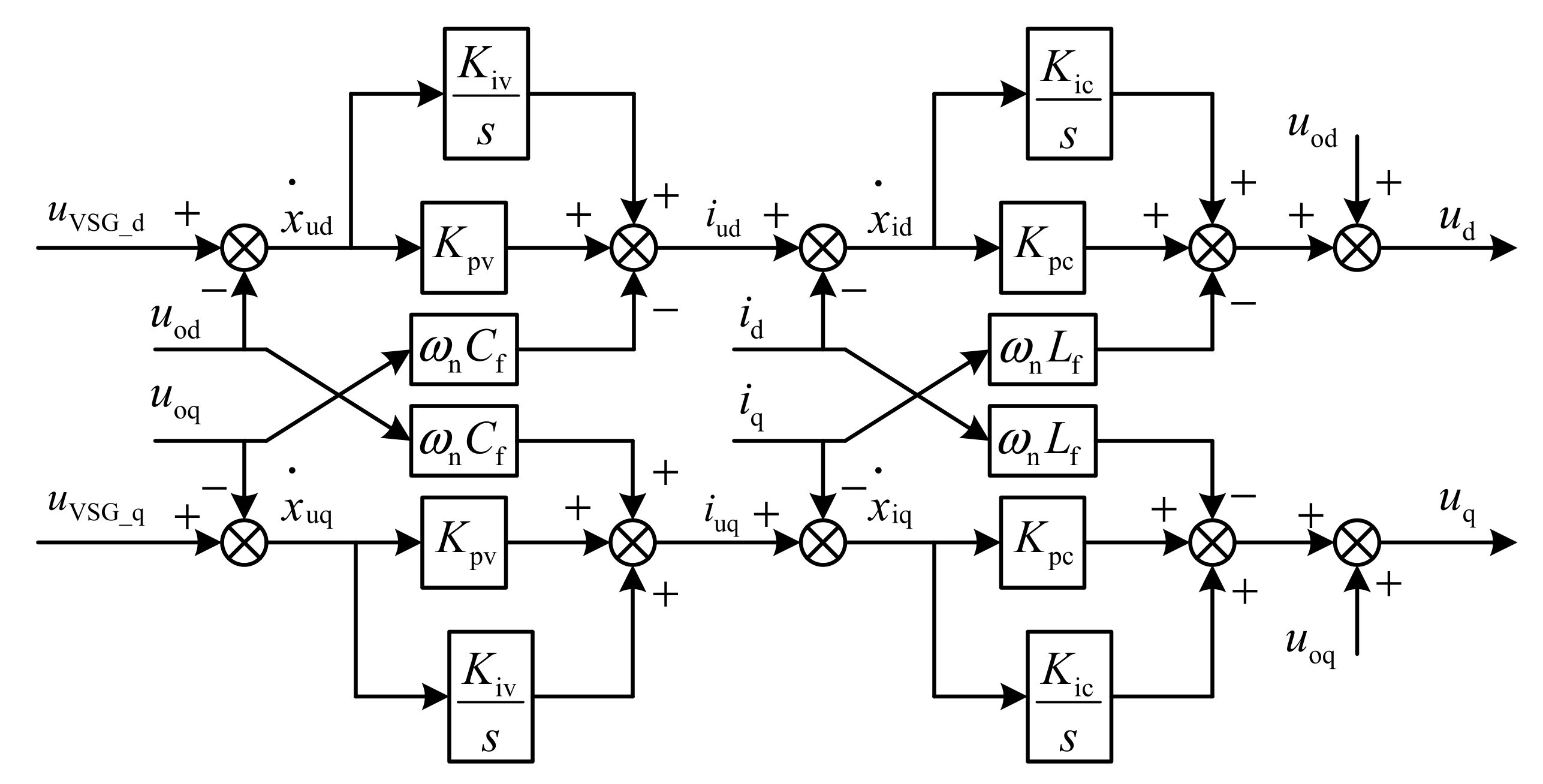
3.3. Small-Signal Model of Voltage and Current Closed Loops

Figure 5 shows the control structure of the voltage outer loop and the current inner loop. In Figure 5, K_pv, K_iv, K_pc, and K_ic are the PI controller parameters of the voltage outer loop and the current inner loop, respectively.

According to Figure 5, the small-signal model of volage and current closed loops is expressed by (6).

$$\left\{\begin{array}{l}\Delta i_{\mathrm{ud}}=K_{\mathrm{iv}}\Delta x_{\mathrm{ud}}+K_{\mathrm{pv}}\Delta u_{\mathrm{VSG}\_\mathrm{d}}-K_{\mathrm{pv}}\Delta u_{\mathrm{od}}-{\omega }_{\mathrm{n}}{C}_{\mathrm{f}}\Delta u_{\mathrm{oq}}\\ \Delta i_{\mathrm{uq}}=K_{\mathrm{iv}}\Delta x_{\mathrm{uq}}+K_{\mathrm{pv}}\Delta u_{\mathrm{VSG}\_\mathrm{q}}-K_{\mathrm{pv}}\Delta u_{\mathrm{oq}}+{\omega }_{\mathrm{n}}{C}_{\mathrm{f}}\Delta u_{\mathrm{od}}\\ \Delta u_{\mathrm{d}}=K_{\mathrm{ic}}\Delta x_{\mathrm{id}}+K_{\mathrm{pc}}\Delta i_{\mathrm{ud}}-K_{\mathrm{pc}}\Delta i_{\mathrm{d}}-{\omega }_{\mathrm{n}}{L}_{\mathrm{f}}\Delta i_{\mathrm{q}}+\Delta u_{\mathrm{od}}\\ \Delta u_{\mathrm{q}}=K_{\mathrm{ic}}\Delta x_{\mathrm{iq}}+K_{\mathrm{pc}}\Delta i_{\mathrm{uq}}-K_{\mathrm{pc}}\Delta i_{\mathrm{q}}+{\omega }_{\mathrm{n}}{L}_{\mathrm{f}}\Delta i_{\mathrm{d}}+\Delta u_{\mathrm{oq}}\end{array}\right.,$$

(6)

where x_ud, x_uq, x_id, and x_iq are the intermediate state variables to describe the dynamic characteristics of PI controller in voltage and current closed loops. The corresponding state equation is calculated by (7).

$$\left\{\begin{array}{l}\frac{\mathrm{d}{x}_{\mathrm{ud}}}{\mathrm{d}t}=u_{\mathrm{VSG}\_\mathrm{d}}-u_{\mathrm{od}}\\ \frac{\mathrm{d}{x}_{\mathrm{uq}}}{\mathrm{d}t}=u_{\mathrm{VSG}\_\mathrm{q}}-u_{\mathrm{oq}}\\ \frac{\mathrm{d}{x}_{\mathrm{id}}}{\mathrm{d}t}=i_{\mathrm{ud}}-i_{\mathrm{d}}\\ \frac{\mathrm{d}{x}_{\mathrm{iq}}}{\mathrm{d}t}=i_{\mathrm{uq}}-i_{\mathrm{q}}\end{array}\right..$$

(7)

The small-signal model is summarized by (8).

$$\frac{\mathrm{d}}{\mathrm{d}t}\left[\begin{array}{l}\Delta x_{\mathrm{udq}}\\ \Delta x_{\mathrm{idq}}\end{array}\right]=A_1\left[\begin{array}{l}\Delta u_{\mathrm{odq}}\\ \Delta i_{\mathrm{dq}}\end{array}\right]+B_1{\left[\begin{array}{lll}\Delta i_{\mathrm{dq}}& \Delta u_{\mathrm{odq}}& \Delta i_{\mathrm{odq}}\end{array}\right]}^T,$$

(8)

where

$$A_1=\left[\begin{array}{cccc}1& 0& 0& 0\\ 0& 1& 0& 0\\ 0& 0& 1& 0\\ 0& 0& 0& 1\end{array}\right],B_1=\left[\begin{array}{cccccc}0& 0& -1& 0& 0& 0\\ 0& 0& 0& -1& 0& 0\\ -1& 0& 0& 0& 0& 0\\ 0& -1& 0& 0& 0& 0\end{array}\right].$$

3.4. Small-Signal Model of Power Grid

The grid voltage and frequency are modeled by (9).

$$\left\{\begin{array}{l}{u}_{\mathrm{gd}}=E_{\mathrm{g}}\sin {\delta }_{\mathrm{g}}\\ u_{\mathrm{gq}}=E_{\mathrm{g}}\cos {\delta }_{\mathrm{g}}\\ {\dot{\delta }}_g={\omega }_{\mathrm{g}}-\omega \end{array}\right.,$$

(9)

where E_g is the voltage amplitude of the AC power grid, ω_g is the angular frequency of the AC power grid, and δ_g is the phase difference between the AC grid voltage and the d axis of the reference coordinate system.

Linearizing Equation (9), the small-signal model of the power grid is shown in (10).

$$\left\{\begin{array}{l}\Delta u_{\mathrm{gd}}=E_{\mathrm{g}}\cos {\delta }_{\mathrm{g}0}\Delta {\delta }_{\mathrm{g}}\\ \Delta u_{\mathrm{gq}}=-E_{\mathrm{g}}\sin {\delta }_{\mathrm{g}0}\Delta {\delta }_{\mathrm{g}}\\ \Delta {\dot{\delta }}_{\mathrm{g}}=-\Delta \omega \end{array}\right..$$

(10)

Based on the above small-signal models, the overall small-signal model of the single VSG grid-connected system can be obtained by (11).

$$\Delta \dot{x}=A\Delta x,$$

(11)

where Δx = [Δx₁,Δδ_g]^T is the system state variable, and Δx₁ = [Δω,Δi_dq,Δu_odq,Δi_odq,Δx_udq,Δx_idq]^T.

4. Small-Signal Model of Multi-VSG Grid-Connected System

For a multi-VSG grid-connected system, it is necessary to transform the coordinate system of all VSGs to a common coordinate system. For the convenience of analysis, the dq coordinate system of the first VSG is selected as the system common reference coordinate system, and the transformation diagrams of other VSGs are shown in Figure 6. We assume that the output voltage of the i-th VSG is ahead of that of the first VSG electrical angle θ_i, as shown in (12).

$${\theta }_i={\displaystyle \int ({\omega }_i-{\omega }_1)}dt.$$

(12)

The following is the corresponding linearized equation of (12):

$$\Delta {\dot{\theta }}_i=\Delta {\omega }_i-\Delta {\omega }_1.$$

(13)

Thus, the small-signal output current ∆i_oDQi of the i-th inverter on the common coordinate system and the output voltage ∆u_bdqi on its own coordinate system can be obtained by Equations (14) and (15), respectively.

$$\Delta i_{\mathrm{oDQ}}{}_i=T_{\mathrm{s}i}\Delta i_{\mathrm{odq}i}+T_{\mathrm{c}i}\Delta {\theta }_i.$$

(14)

$$\Delta u_{\mathrm{bdq}i}=T_{\mathrm{s}i}^{-1}\Delta u_{\mathrm{bDQ}i}+T_{\mathrm{u}i}^{-1}\Delta {\theta }_i.$$

(15)

According to the transformation of the reference coordinate system, the small-signal model of the multi-VSG system is expressed by (16).

$$\Delta {\dot{x}}_i=A_i\Delta x_i,$$

(16)

where Δx_i = [Δx₁,θ₂,Δx₁,…,θ_i,Δx_i,Δδ_g]^T.

5. Stability Analysis Based on Eigenvalues

5.1. Stability Analysis of Single-VSG Grid-Connected System

5.1.1. Oscillation Mode Analysis of Single-VSG System

According to the single-VSG grid-connected small-signal model in Equation (11), all eigenvalues of the system are obtained based on the parameters in

Table 1. Single-VSG system parameters.

Parameter	Value	Parameter	Value
Rf/Ω	0.2	Lc/mH	1.8
Lf/mH	3.2	Pref/kW	10
Cf/μF	100	Qref/var	0
Rc/Ω	0.1	J/kg·m2	10
D/N·m·s·rad−1	70	Kd	30
Kq	0.0005

and

Table 2. Steady-state operating points of the single-VSG system.

Parameter	Value	Parameter	Value
Id/A	21.27	Iod/A	1.8
Iq/A	11.66	Ioq/A	10
Uod/V	311.3	ω0/rad·s−1	314.2
Uoq/V	4.401

. Subsequently, the oscillation mode of the single-VSG grid-connected system and the influence of parameter changes at the steady-state operation point on the small-signal stability of the system are analyzed.

The system eigenvalues are shown in

Table 3. Single-VSG system eigenvalues.

Eigenvalue	Real Part	Imaginary Part	Oscillation Frequency/Hz	Damping Ratio	Dominant Related State Variables
λ1–2	−3.15	±6.89	1.09	0.42	id, iq, xud, xuq
λ3–4	−30.21	±22.38	3.56	0.80	id, iq, xid, xiq
λ5–6	−6.84	±39.03	6.21	0.17	ω, δg,
λ7–8	−418.3	±349.98	55.73	0.77	iod, ioq
λ9–10	−217.04	±4797.2	763.89	0.045	id, iq, uod, uoq
λ11–12	−1000	±5525.8	879.90	0.18	id, iq, uod, uoq

. The system has twelve eigenvalues, corresponding to six oscillation modes. The eigenvalues of the system are in the left half plane of the complex plane, indicating that the system is stable. The distance between the eigenvalues λ_11–12 and the imaginary axis is much greater than other eigenvalues, which has little influence on the system stability and can be ignored. The eigenvalues λ_1–2 have the smallest oscillation frequency and are closest to the imaginary axis. An oscillation attenuation mode is presented for the system.

The following mainly considers the influence of active power outer loop controller parameters and connecting line parameters on system stability, especially the influence of virtual moment of inertia and virtual damping coefficient on system small-signal stability.

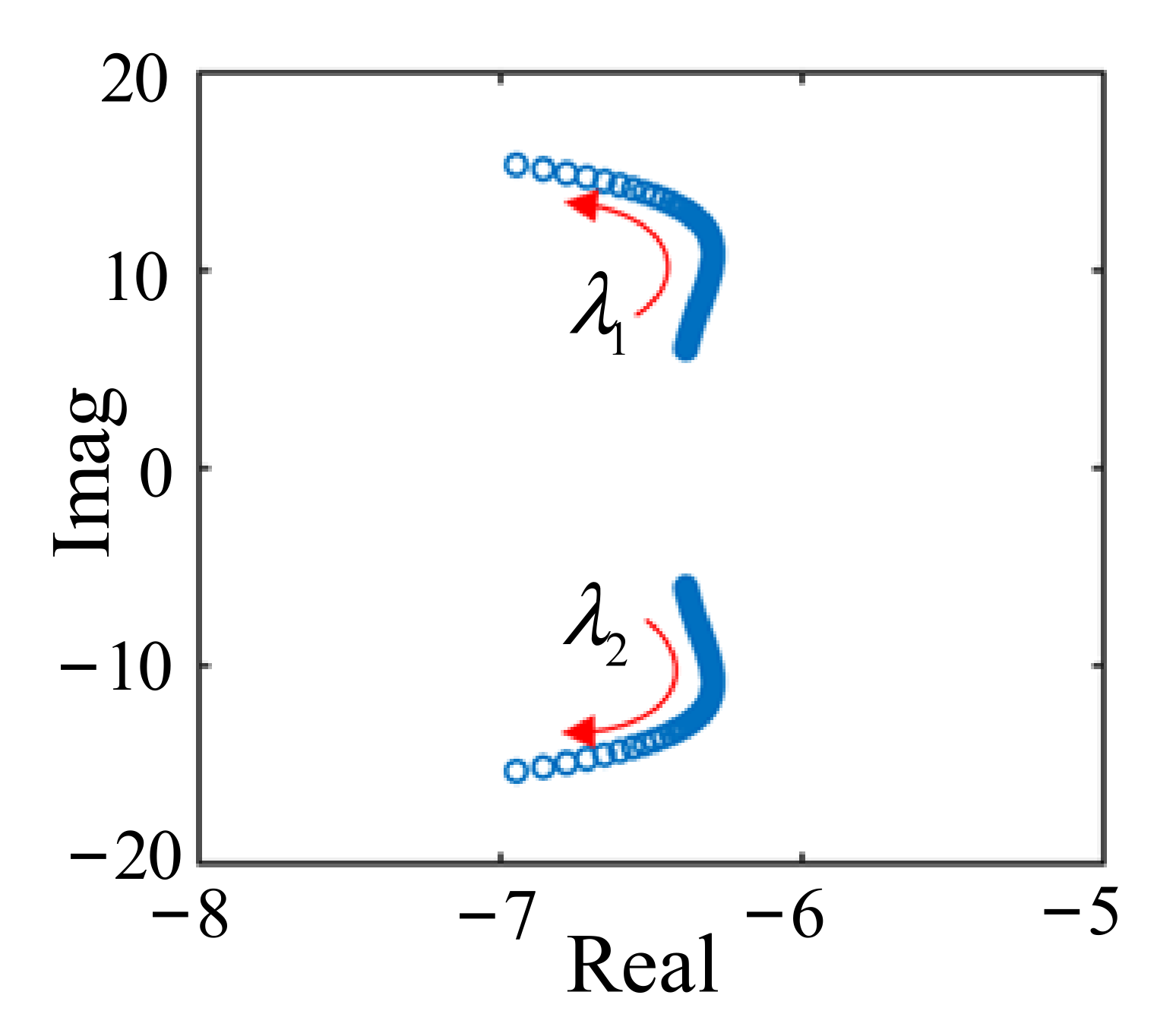
5.1.2. Influence of Active Power Loop Control Parameters on Eigenvalues

The control parameters of active power loop include the virtual moment of inertia J and the virtual damping coefficient D. The eigenvalue trajectories with the parameter changes are shown in Figure 7.

When the virtual inertia changes J = 3.5→14, other parameters remain unchanged, and the influence on the eigenvalues λ_1–2 of the oscillation attenuation mode is shown in Figure 7a. With the increase in virtual inertia J, the eigenvalues λ_1–2 move rapidly towards the imaginary axis, the damping ratios of the corresponding oscillation attenuation mode decrease rapidly, the oscillation frequency decreases slightly, and the system stability worsens. Shown in Figure 7b is the influence on the eigenvalues λ_1–2 of the oscillation attenuation mode when the virtual damping coefficient changes D = 70→130. With the increase in virtual damping coefficient D, the eigenvalues λ_1–2 move to the left of the complex plane, and the movement speed away from the imaginary axis is much higher than that away from the real axis. The damping ratio of the corresponding oscillation attenuation mode increases, the overshoot will gradually decrease, the oscillation frequency will increase slightly, and the system stability will be improved.

5.1.3. Influence of Resistance Inductance Ratio of Connecting Line on Eigenvalues

The resistance inductance ratio r of the connecting line on the grid side is defined by (17).

$$r=\frac{R_{\mathrm{c}}}{100\pi L_{\mathrm{c}}}.$$

(17)

The resistance inductance ratio r of the connecting line on the grid side represents the voltage level of the grid. The influence of voltage level change on the eigenvalues is shown in Figure 8. With the increase in r, the speed of the eigenvalues λ_1–2 moving to the upper left of the coordinate system and away from the imaginary axis is much higher than that of the real axis, and the damping ratio of the system increases.

5.2. Stability Analysis of Multi-VSG System

5.2.1. Oscillation Mode Analysis of Multi-VSG System

To analyze the stability of a multi-VSG system, I = 2 is taken as an example. The corresponding structure diagram of a two-VSG system is shown in Figure 9.

The system parameters and steady-state operation points are shown in

Table 4. Multi-VSG system parameters.

Parameter	Value	Parameter	Value
Rf1,2/Ω	0.2	Pref1/kW	10
Lf1,2/mH	3.2	J1,2	10
Cf1,2/μF	100	D1,2	70
Rc1,2/Ω	0.1	Kd1,2	30
Lc1,2/mH	1.8	Kq1,2	0.0005
Pref2/kW	13	Kpv	2
Kiv	50	Kpc	7
Kic	75

and

Table 5. Steady-state operating points of the multi-VSG system.

Parameter	Value	Parameter	Value
Id1/A	21.24	Id2/A	27.64
Uod1/V	311.70	Uod2/V	311.90
Iod1/A	21.38	Iod2/A	27.78
Iq1/A	13.36	Iq2/A	14.05
Uoq1/V	4.41	Uoq2/V	4.41
Ioq1/A	3.43	Ioq2/A	4.12

. We bring the parameters in Table 4 and Table 5 into Equation (16) to obtain all eigenvalues, as shown in

Table 6. Multi-VSG system eigenvalues.

Eigenvalue	Real Part	Imaginary Part	Oscillation Frequency/Hz	Damping Ratio	Dominant Related State Variables
λ1–2	−55129.01	±319.24	50.03	0.99	iodq1, iodq2
λ3–4	−1268.41	±4247.55	676.36	0.29	uodq1, uodq2, idq1, idq2
λ5–6	−937.89	±1537.41	244.81	0.52	uodq1, uodq2, iodq1, iodq2
λ7–8	−41.48	±848.78	135.16	0.05	uodq1, uodq2, iodq1, iodq2
λ9–10	−33.72	±3247.69	517.15	0.01	uodq1, uodq2, idq1, idq2
λ11–12	−29.00	±2340.81	372.74	0.02	uodq1, uodq2, idq1, idq2
λ13–14	−122.46	±542.93	86.45	0.22	iodq1, iodq2
λ15–16	−69.26	±331.68	52.81	0.21	iodq1, iodq2, idq1
λ17–18	−60.38	±336.65	53.6	0.18	iodq1, iodq2, idq2
λ19–20	−4.03	±1.12	0.18	0.96	ω1, ω2
λ21–22	−3.2	±3.17	0.50	0.71	θ2, ω1, ω2, δg
λ23–24	−4.39	±2.17	0.35	0.89	θ2, ω1, ω2

.

In Table 6, the two-VSG system has 24 eigenvalues, which are distributed in high-, medium-, and low-frequency bands, corresponding to 12 oscillation modes of the system. All eigenvalues are in the left half plane of the complex plane. The two-VSG system is statically stable. Since the eigenvalues λ_1–2 are the farthest from the imaginary axis among all eigenvalues and have the largest damping ratio, their influences on the stability of the system can be ignored. The eigenvalues λ_3–12, λ_13–18, and λ_19–24 correspond to high-, medium-, and low-frequency bands, respectively. By calculating the participation factor, high- and medium-frequency eigenvalues λ_3–18 are mainly related to the inverter output current controlled by the VSG and the state variables of the LC filter. Low-frequency eigenvalues λ_19–24 are related to the virtual angular frequency of each VSG and the phase difference with reference coordinates.

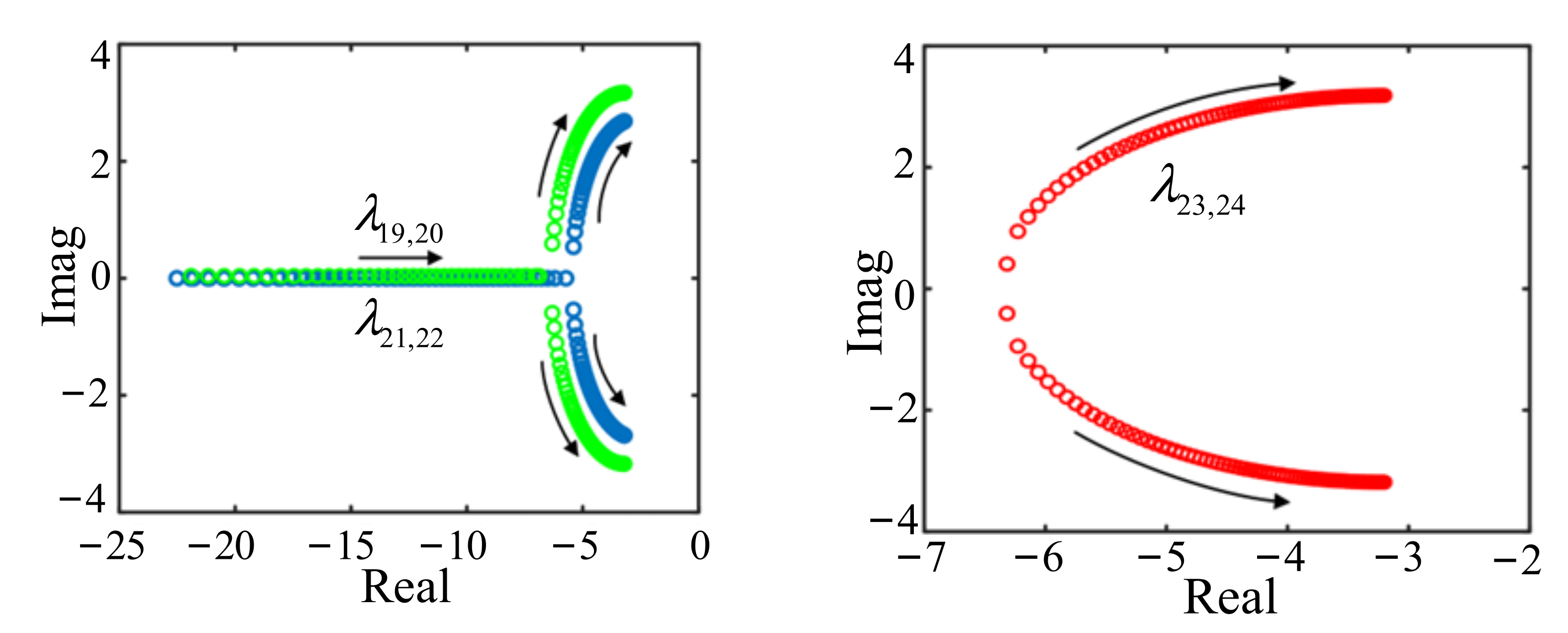
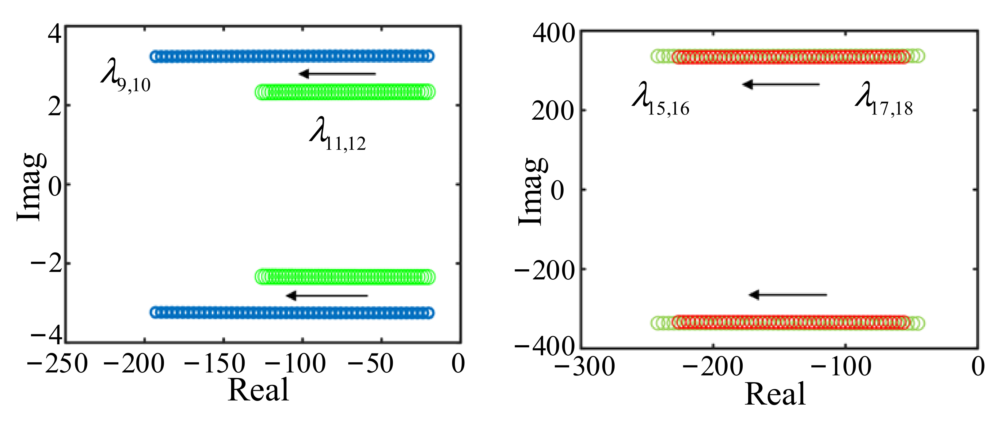
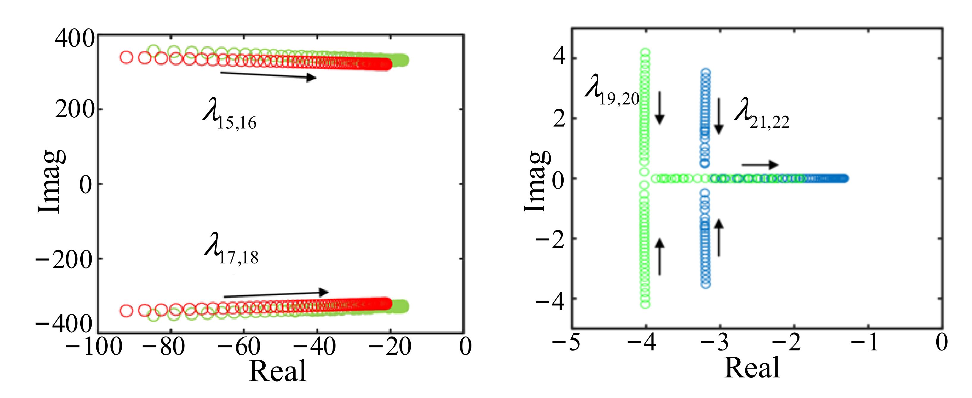
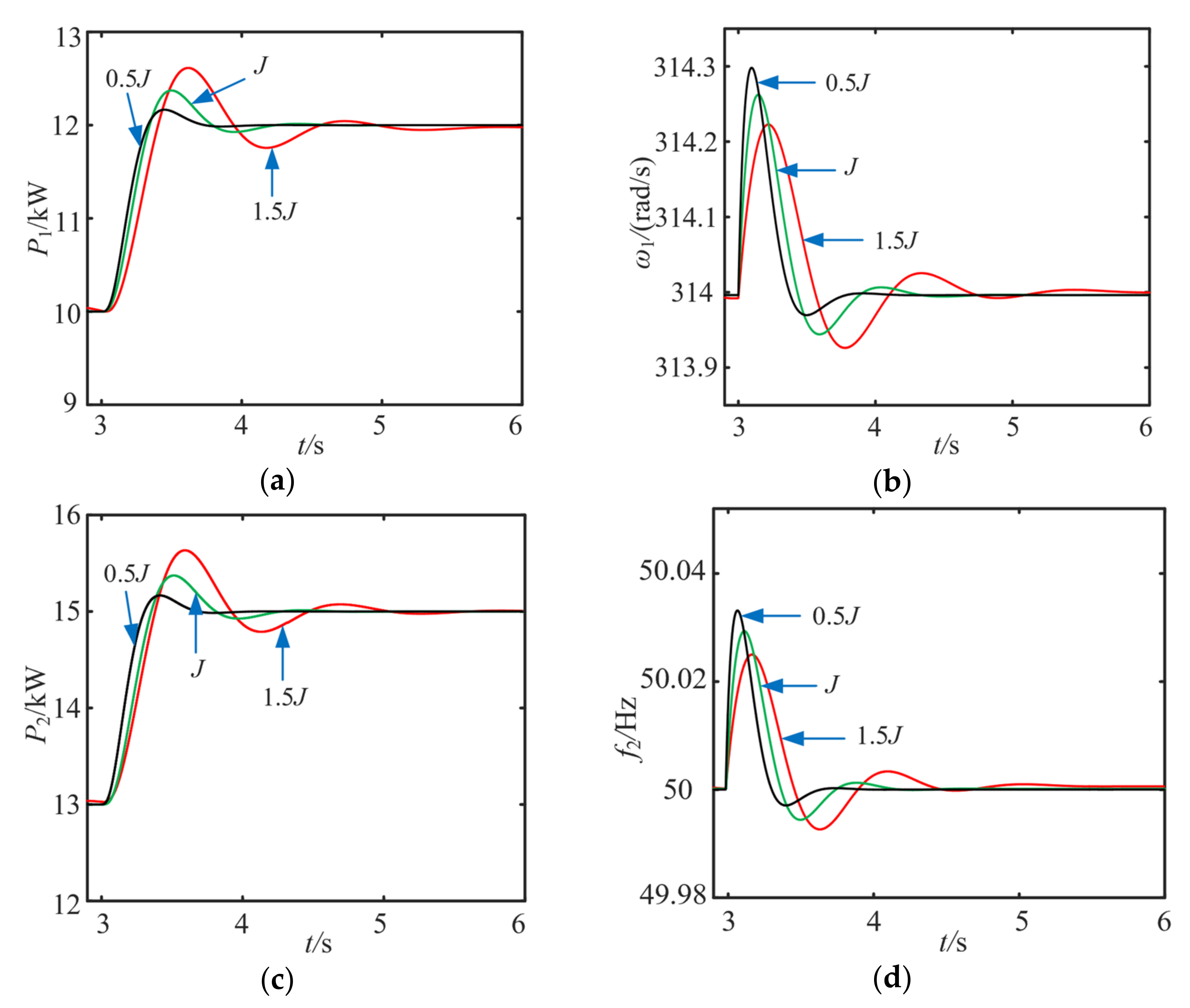
5.2.2. Influence of Virtual Inertia on Eigenvalues

The change trends of the eigenvalue trajectories of the system with the increase in the virtual inertia of each VSG (J = 3.5→14) are shown in Figure 10. The eigenvalues λ_19–24 move towards the imaginary axis, and their impact on the system stability cannot be ignored. The eigenvalues λ_19–20 (green trajectories in the figure) and the eigenvalues λ_21–22 (blue trajectories in the figure) have the same change trend. When the virtual moment of inertia J increases to a certain extent, the eigenvalues move away from the real axis and close to the imaginary axis, and the speed away from the real axis is greater than the speed close to the imaginary axis. The eigenvalues λ_23–24 monotonically and rapidly move away from the real axis and close to the imaginary axis, and the speed close to the imaginary axis is greater than that away from the real axis. The damping of the corresponding oscillation attenuation mode decreases rapidly, and the system stability will worsen.

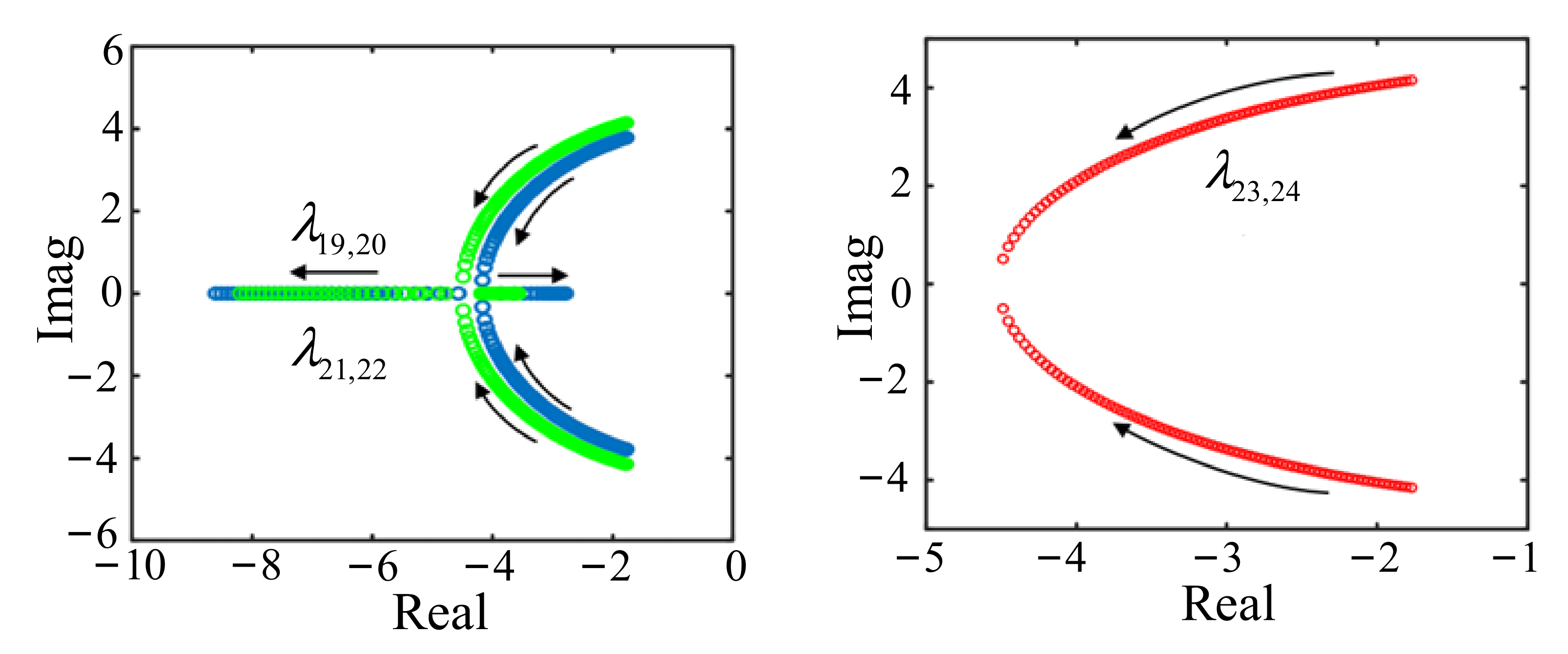
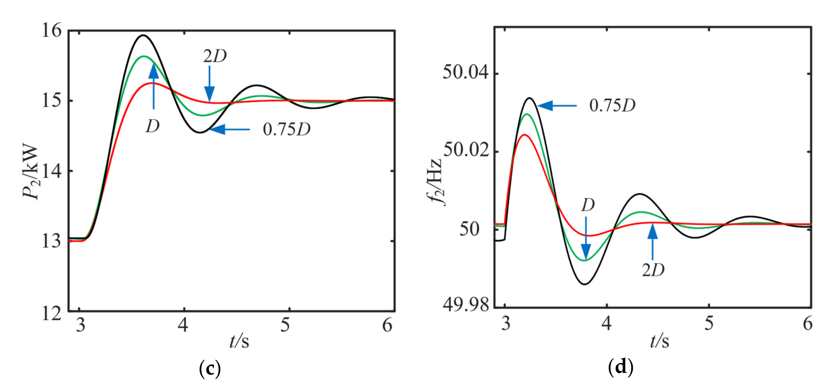
5.2.3. Influence of Damping Coefficient on Eigenvalues

The influence of the change in damping coefficient on the eigenvalue trajectories of the system is shown in Figure 11. With the increase in the damping coefficient of each VSG(D = 70→130), the system eigenvalues in the low-frequency band λ_19–24 move to the left of the complex plane. The imaginary parts of the eigenvalues λ_19–20 (green trajectories in the figure) and λ_21–22 (blue trajectories in the figure) gradually move close to the real axis, and the oscillation frequency of the corresponding oscillation attenuation mode decreases. When the damping coefficient D increases to a certain extent, they will move away from the imaginary axis and close to the imaginary axis along the real axis. The eigenvalues λ_23–24 quickly move away from the imaginary axis and close to the real axis. The damping of the corresponding oscillation attenuation mode increases and the system stability will be improved.

5.2.4. Influence of Line Resistance on Eigenvalues

The influence of the line resistance changes on the eigenvalue trajectories of the system is shown in Figure 12. When the line resistance R_c gradually increases from 0.025 Ω to 1 Ω, and other parameters remain unchanged, the high-frequency eigenvalues λ_9–12 and intermediate-frequency eigenvalues λ_15–18 move to the left of the complex plane. The moving speeds of the eigenvalues λ_9–10 are greater than those of the eigenvalues λ_11–12. However, the moving speed of the eigenvalues λ_15–16 (yellow trajectories in the figure) is basically the same as that of the eigenvalues λ_17–18 (red trajectories in the figure), their imaginary part is basically unchanged, the real part is gradually reduced, and the damping of the corresponding oscillation attenuation mode increases. Therefore, increasing the line resistance can increase the system damping and improve the system stability.

5.2.5. Influence of Line Inductance on Eigenvalues

The influence of line inductance changes on the system eigenvalue trajectories is shown in Figure 13 (yellow trajectories in the figure are eigenvalues λ_15–16, red trajectories in the figure are eigenvalues λ_17–18). When the line inductance changes L_c = 0.36 mH→15 mH, other parameters remain unchanged, and the intermediate-frequency eigenvalues λ_15–18 move to the right of the complex plane. The imaginary parts of the eigenvalues λ_15–18 decrease slowly, the real parts increase rapidly, and the intermediate frequency damping decreases. The low-frequency eigenvalues λ_19–22 move towards the direction close to the real axis, the real parts of the eigenvalues are basically unchanged, the imaginary parts decrease rapidly, and the oscillation frequency decreases significantly. When the line inductance increases to a certain extent, the eigenvalues move along the right side of the real axis complex plane and quickly approach the imaginary axis, and the low-frequency damping of the system decreases. Increasing the line inductance can reduce the system damping, which is not conducive to the system’s stability.

6. Time Domain Simulation Verification and Result Discussion

6.1. Simulation of Single-VSG Grid-Connected System

To verify the correctness of the analysis of the above variable parameters on the change law of eigenvalue trajectories, a time domain simulation model of a VSG grid-connected system was built, as shown in Figure 1. The system parameters under the initial operating conditions are shown in Table 1. When t = 3 s, the system load is increased by 2 kW.

Under the initial operating conditions, the system parameters are set as the references. The ratios of the virtual inertia J, the virtual damping coefficient D, and the resistance inductance ratio r of the connecting lines to their corresponding references are 0.5, 1, and 1.5, respectively.

Virtual inertia J has a significant influence on the active power and virtual angular frequency of the system. As the virtual inertia gradually increases, the overshoot in active power increases, while the overshoot in virtual angular frequency decreases, and the response time and decay oscillation time of active power and virtual angular frequency are extended.

As the virtual damping coefficient increases, the response times of active power and virtual corner frequency remain the same. However, their overshoot is decreased, the oscillation time becomes shorter, and the decay oscillation time becomes faster.

As the resistive inductance ratio r increases, the response times of active power and virtual angular velocity increase, and the decay oscillation time decreases. The overshoot of active power is decreased, but the overshoot of virtual angular frequency is increased.

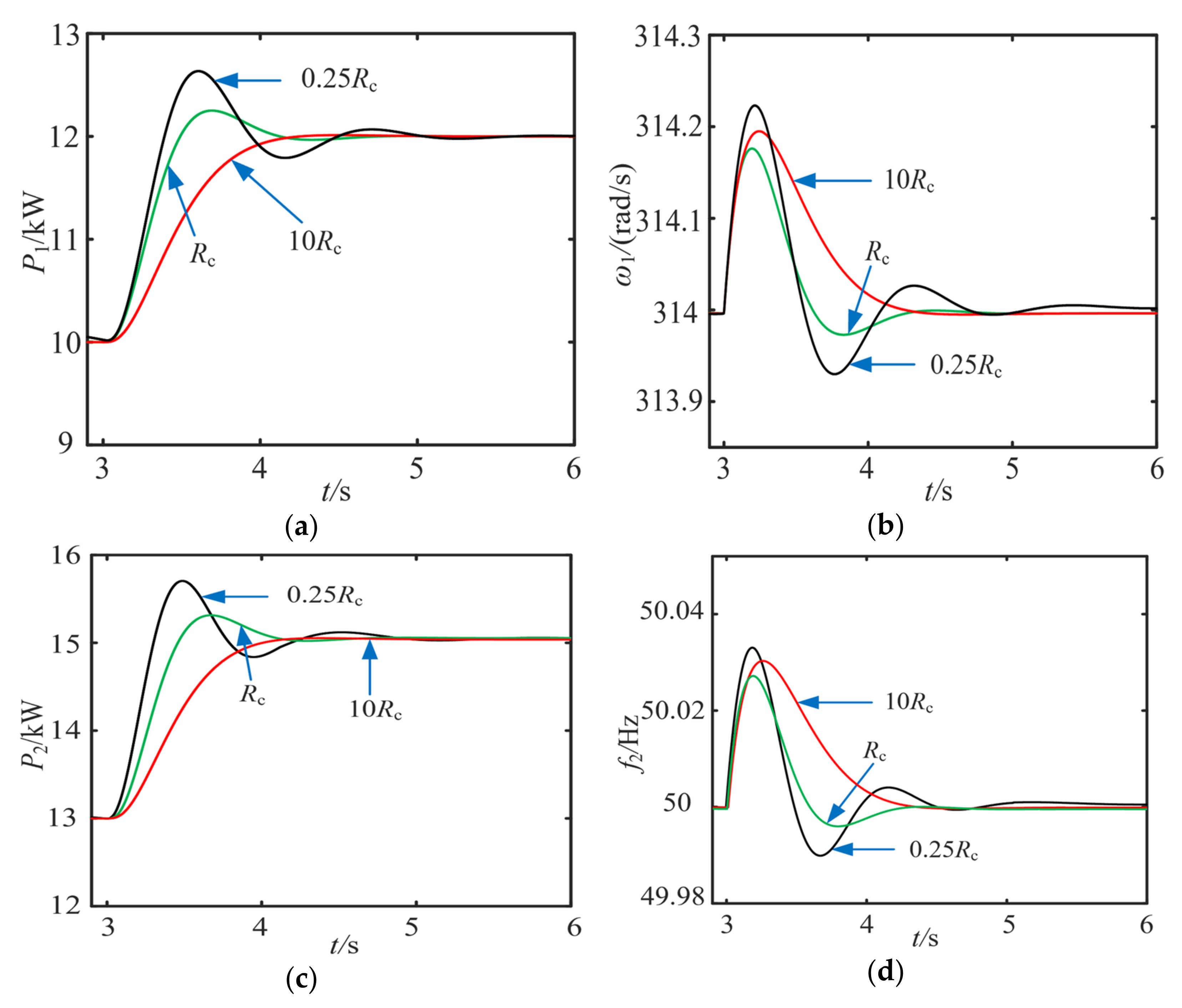
6.2. Simulation of Multi-VSG Grid-Connected System

The time domain simulation model of the two-VSG grid-connected system is built to verify the correctness of the analysis of the influence of the above variable parameters (J, D, R_c, L_c) on the system stability. With the same other parameters (as shown in Table 4), when the power is disturbed, the response simulation waveforms under different virtual moments of inertia, virtual damping coefficients, line resistances, and line inductances are shown in Figure 14, Figure 15, Figure 16 and Figure 17, respectively.

As can be seen from Figure 14 and Figure 15, increasing the virtual inertia J or decreasing the virtual damping coefficient D will make the system unstable under a power disturbance. Increasing the virtual inertia J influences the number of oscillations of active power and frequency under power disturbance, increasing the regulation time of the system. Increasing the virtual damping coefficient D reduces the amplitude of oscillations of active power and frequency and shortens the time for the system to reach stability.

In Figure 16 and Figure 17, reducing the line resistance R_c or increasing the line inductance L_c will deteriorate the system stability. Reducing the line resistance R_c will increase the overshoot of active power, and the adjustment time of active power and frequency will be increased. Increasing the line inductance L_c will enlarge the overshoot of active power and reduce the overshoot of frequency.

7. Conclusions

We studied the stability of single-VSG and multi-VSG systems. The influence mechanisms of various parameters on system stability were verified by small-signal models and numerous simulation models. The conclusions are as follows.

(1) In the single-VSG grid-connected system, increasing the virtual moment of inertia will rapidly reduce the damping ratio of the corresponding oscillation attenuation mode and deteriorate the system stability. Increasing the virtual damping coefficient and the resistance inductance ratio of the connecting line will increase the damping ratio and improve the system stability.

(2) In the multi-VSG system, increasing the damping coefficient and line resistance will increase the system damping and improve the system stability. Increasing the virtual moment of inertia and line inductance will reduce the system damping, which is not conducive to the system stability.

We achieved some research results that provide a theoretical reference for the matching and selection of various parameters in VSG single-machine grid-connected systems and multi-VSG parallel grid-connected systems. However, further in-depth research and discussion are still needed:

(1) The influence of grid voltage fluctuation is not considered in the small-signal stability analysis of VSG single-machine and multi-machine parallel systems. When the voltage fluctuates, the transient stability of VSG needs further study.

(2) This paper mainly verifies the theoretical analysis through time domain simulation, and a semi-physical test platform based on theory and simulation is necessary to further prove the effectiveness of the results.

References

1. Du, W.J.; Fu, Q.; Wang, H.F. Damping torque analysis of DC voltage stability of an MTDC network for the wind power delivery. IEEE Trans. Power Deliv. 2020, 35, 324–338. [Google Scholar] [CrossRef]
2. Liu, C.L.; Li, D.Z.; Wang, L.C.; Li, L.; Wang, K. Strong robustness and high accuracy remaining useful life prediction on supercapacitors. APL Mater. 2022, 10, 061106. [Google Scholar] [CrossRef]
3. Yi, Z.X.; Zhao, K.; Sun, J.R.; Wang, L.; Wang, K.; Ma, Y. Prediction of the remaining useful life of supercapacitors. J. Power Sources 2022, 2022, 7620382. [Google Scholar] [CrossRef]
4. Li, D.Z.; Li, S.; Zhang, S.; Sun, J.; Wang, L.; Wang, K. Aging state prediction for supercapacitors based on heuristic kalman filter optimization extreme learning machine. Energy 2022, 250, 123773. [Google Scholar] [CrossRef]
5. Zarifakis, M.; Coffey, W.T.; Kalmykov, Y.P. Active damping of power oscillations following frequency changes in low inertia power systems. IEEE Trans. Power Syst. 2019, 34, 4984–4992. [Google Scholar] [CrossRef]
6. Wu, W.H.; Chen, Y.D.; Zhou, L.M.; Luo, A.; Zhou, X.P.; He, Z.X.; Yang, L.; Xie, Z.W.; Liu, J.M.; Zhang, M.M. Sequence impedance modeling and stability comparative analysis of voltage-controlled VSGs and current-controlled VSGs. IEEE Trans. Ind. Electron. 2019, 66, 6460–6472. [Google Scholar] [CrossRef]
7. Khajehoddin, S.A.; Karimi-Ghartemani, M.; Ebrahimi, M. Grid-supporting inverters with improved dynamics. IEEE Trans. Ind. Electron. 2019, 65, 3655–3667. [Google Scholar] [CrossRef]
8. Zhong, Q.C.; Weiss, G. Synchronverters: Inverters that mimic synchronous generators. IEEE Trans. Ind. Electron. 2011, 58, 1259–1267. [Google Scholar] [CrossRef]
9. Liu, J.; Miura, Y.; Bevrani, H.; Ise, T. Enhanced virtual synchronous generator control for parallel inverters in microgrids. IEEE Trans. Smart Grid 2017, 8, 2268–2277. [Google Scholar] [CrossRef]
10. Xu, Y.; Nian, H.; Hu, B. Impedance modeling and stability analysis of VSG controlled type-IV wind turbine system. IEEE Trans. Energy Convers. 2021, 36, 3438–3448. [Google Scholar] [CrossRef]
11. Baruwa, M.; Fazeli, M. Impact of virtual synchronous machines on low-frequency oscillations in power systems. IEEE Trans. Power Syst. 2021, 36, 1934–1946. [Google Scholar] [CrossRef]
12. Shuai, Z.K.; Shen, C.; Liu, X.; Li, Z.; Shen, Z.J. Transient angle stability of virtual synchronous generators using lyapunov’s direct method. IEEE Trans. Smart Grid 2019, 10, 4648–4661. [Google Scholar] [CrossRef]
13. Xiong, X.L.; Wu, C.; Blaabjerg, F. Effects of virtual resistance on transient stability of virtual synchronous generators under grid voltage sag. IEEE Trans. Ind. Electron. 2022, 69, 4754–4764. [Google Scholar] [CrossRef]
14. Liu, H.; Sun, D.W.; Song, P.; Cheng, X.; Zhao, F.; Tian, Y. Influence of virtual synchronous generators on low frequency oscillations. CSEE J. Power Energy Syst. 2022, 8, 1029–1038. [Google Scholar]
15. Wang, G.Y.; Fu, L.J.; Hu, Q.; Ma, F.; Liu, C.; Lin, Y. Low frequency oscillation analysis of VSG grid-connected system. In Proceedings of the 2021 3rd Asia Energy and Electrical Engineering Symposium (AEEES), Chengdu, China, 26–29 March 2021; pp. 631–637. [Google Scholar]
16. Qin, B.S.; Xu, Y.H.; Yuan, C.; Jia, J. A unified method of frequency oscillation characteristic analysis for multi-VSG grid-connected system. IEEE Trans. Power Deliv. 2022, 37, 279–289. [Google Scholar] [CrossRef]
17. Alipoor, J.; Miura, Y.; Ise, T. Stability assessment and optimization methods for microgrid with multiple VSG units. IEEE Trans. Smart Grid 2018, 9, 1462–1471. [Google Scholar] [CrossRef]
18. Choopani, M.; Hosseinian, S.H.; Vahidi, B. New transient stability and LVRT improvement of multi-VSG grids using the frequency of the center of inertia. IEEE Trans. Power Syst. 2020, 35, 527–538. [Google Scholar] [CrossRef]
19. Fu, S.Q.; Sun, Y.; Li, L.; Liu, Z.; Han, H.; Su, M. Power oscillation suppression of multi-VSG grid via decentralized mutual damping control. IEEE Trans. Ind. Electron. 2022, 69, 10202–10214. [Google Scholar] [CrossRef]
20. Shi, M.X.; Chen, X.; Zhou, J.Y.; Chen, Y.; Wen, J.Y.; He, H. Frequency restoration and oscillation damping of distributed VSGs in microgrid with low bandwidth communication. IEEE Trans. Smart Grid 2021, 12, 1011–1021. [Google Scholar] [CrossRef]
21. Hu, Y.; Bu, S.Q.; Zhang, X.; Chung, C.Y.; Cai, H. Connection between damping torque analysis and energy flow analysis in damping performance evaluation for electromechanical oscillations in power systems. J. Mod. Power Syst. Clean Energy 2022, 10, 19–28. [Google Scholar] [CrossRef]
Figure 1. Topology diagram of VSG.
Energies 15 07158 g001
Figure 2. Structure block diagram of VSG governor control.
Energies 15 07158 g002
Figure 3. Structure of virtual moment of inertia control.
Energies 15 07158 g003
Figure 4. The block diagram of virtual excitation control.
Energies 15 07158 g004
Figure 5. Block diagram of voltage–current double-loop control.
Energies 15 07158 g005
Figure 6. Schematic diagram of reference coordinate system transformation of multi-VSG system.
Energies 15 07158 g006
Figure 7. The eigenvalue trajectories under different active power control parameters. (a) Eigen-value trajectories of the system under different inertias. (b) Eigenvalue trajectories of the system under different damping coefficients.
Energies 15 07158 g007
Figure 8. Eigenvalue trajectories under different resistance inductance ratios of connecting lines.
Energies 15 07158 g008
Figure 9. Structure diagram of a two-VSG system.
Energies 15 07158 g009
Figure 10. Eigenvalue trajectories of system under different virtual inertias.
Energies 15 07158 g010
Figure 11. Eigenvalue trajectories of the system under different damping coefficients.
Energies 15 07158 g011
Figure 12. Eigenvalue trajectories of the system under different line resistances.
Energies 15 07158 g012
Figure 13. Eigenvalue trajectories of the system under different line inductances.
Energies 15 07158 g013
Figure 14. Simulation waveforms with different virtual inertias: (a) active power of VSG1; (b) virtual angular frequency of VSG1; (c) active power of VSG2; (d) frequency of VSG2.
Energies 15 07158 g014
Figure 15. Simulation waveforms with different damping coefficients: (a) active power of VSG1; (b) virtual angular frequency of VSG1; (c) active power of VSG2; (d) frequency of VSG2.
Energies 15 07158 g015aEnergies 15 07158 g015b
Figure 16. Simulation waveforms with different line resistances: (a) active power of VSG1; (b) virtual angular frequency of VSG1; (c) active power of VSG2; (d) frequency of VSG2.
Energies 15 07158 g016
Figure 17. Simulation waveforms with different line inductances: (a) active power of VSG1; (b) virtual angular frequency of VSG1; (c) active power of VSG2; (d) frequency of VSG2.
Energies 15 07158 g017