Piecewise Affine Magnetic Modeling of Permanent-Magnet Synchronous Machines for Virtual-Flux Control

Abstract

Accurate flux linkage magnetic models are essential for virtual-flux controllers in PMSMs. Flux linkage exhibits saturation and cross-saturation at high currents, introducing nonlinearities into the machine model. Virtual-flux controllers regulate the flux of a machine by using field-oriented control, such as model predictive control. In this study, a methodology for creating a piecewise affine flux linkage magnetic model is proposed which locally linearizes the inductance and flux offset of the machine. This method keeps the magnetic model and thus the state-space model of the system linear while capturing the saturation effects, enabling robust controls and efficient operation. The model is created using FEA-simulated data points and verified with experimental datapoints. An algorithm to optimize the model in MTPA and derated operation is presented with an average flux error less than $1\%$ and maximum error less than $3\%$ using only 40 points. This represents a ≈ 1–3% and ≈5–8% reduction in the average and maximum flux errors compared with a regularly gridded model, respectively.

1. Introduction

Permanent magnet synchronous machines (PMSMs) are the machine of choice for high energy density applications due to their high efficiency and mechanical simplicity. The PMSM has seen widespread adoption in the automotive space [1,2], and is a promising candidate for more-electric and all-electric air propulsion drives [3,4].

The controller performance for a PMSM depends on the accuracy of the machine parameters, such as the stator inductances, stator resistance, and permanent magnet (PM) flux. These parameters can change in real time and have dependencies on the temperature, position, and current. The stator resistance increases nonlinearly with the temperature [5], the PM flux can decrease (demagnetize) at high temperatures [6], and the stator inductance saturates in high currents [7]. These variations are typically accounted for using online parameter estimation, offline parameter look-up tables (LUTs), or a combination of the two.

Online parameter estimation uses real-time feedback of the drive system to estimate the parameters. The feedback can include the current, voltage, speed, and position. Online parameter estimation methods include receding horizon estimation [8], recursive least squares [9], neural networks [10], and extended kalman filters [11].

The offline parameter LUTs use the data of the machine from analytical calculations [12], FEA analysis [6,13], and experimentation [14,15] (or any combination) to approximate the parameters given various operating points of the machine. The datapoints are interpolated in various ways to produce various desirable properties depending on the parameter and application.

Online parameter estimation requires more computation time than offline LUTs but is more accurate over the lifetime of the vehicle by detecting degradation and partial faults in the machine [9,11]. Online parameter estimation also requires either more sensors or sensorless techniques [16] than offline LUTs.

The focus of this study is the flux linkage magnetic model (MM) of the PMSM and the modeling of the stator inductance parameters. To build an offline MM, the current and flux values are processed offline, and continuous inductance functions are created using linear interpolation, Hermite spline interpolation [15,17,18], polynomials [13,19], piecewise nonlinear functions [14], nonlinear functions [12,20], or piecewise affine functions [21]. The results of these methods vary greatly in their properties, as summarized in

Table 1. Summary of offline MM linking methods.

Type of Link	Lin.	Bidir.	Cont.	Diff.	Sat.	Cross-Sat. ${}^1$
Linearized Inductance [22,23]	•	•	•	•
Linearly Interpolated LUT			•		•	•
Spline-Interpolated LUT [15,17,18]			•	•	•	•
Polynomial Functions [13,19]			•	•	•	•
Piecewise Nonlinear Function [14]			•	•	•	•
Other Nonlinear Function [12,20]			•	•	•	•
Piecewise Linear (PWA) [21]	•	•	•		•	•

¹ Linear, bidirectional, continuous, differentiable, saturation, and cross-saturation, respectively.

(the MM accuracy for the linearized inductance, spline-interpolated LUT, and piecewise linear methods is shown in Section 5).

Model predictive control (MPC) is desirable for the PMSM for its stability and robustness properties [22,23]. A virtual-flux MPC (VF-MPC) is a type of VF control that requires a linear flux linkage MM to operate effectively. For this reason, typically, VF-MPC for the PMSM uses linearized stator inductances, which have the effect of linearizing the state-space equation. This greatly simplifies the model, reducing the control error and decreasing the computation time. However, this leads to a flux error of up to $30\%$ in full saturation and 5–20% flux error due to cross-saturation [14,15,19,21].

In this study, we propose using piecewise affine (PWA) functions to build the MM of a PMSM machine. This MM allows for the use of VF-MPC while also taking into account the saturation and cross-saturation effects in the MM. The PWA MM is optimized for current operation, derated operation, and MTPA operation. The experimental flux is compared with the FEA-simulated flux to show the accuracy of the MM.

This paper is organized as follows. The PMSM machine model is described in Section 2, and the construction of the PWA MM is shown in Section 3. The optimization of the PWA MM to the full current range, derated range, and MTPA range is presented in Section 4. Analysis via simulated and experimental results is presented in Section 5, and the paper is concluded in Section 6.

2. PMSM Model

The PMSM is a three-phase synchronous machine that can be dynamically described by the state-space model

$$\begin{array}{cccc}\hfill {\dot{\lambda }}_d& =\omega {\lambda }_q+u_d-R_s{i}_d\hfill & \hfill & =\omega {\lambda }_q+{\overline{u}}_d,\hfill \end{array}$$

(1a)

$$\begin{array}{cccc}\hfill {\dot{\lambda }}_q& =-\omega {\lambda }_d+u_q-R_s{i}_q\hfill & \hfill & =-\omega {\lambda }_d+{\overline{u}}_q,\hfill \end{array}$$

(1b)

where ${\lambda }_d$ and ${\lambda }_q$ are the q-axis and d-axis stator flux linkages, respectively, $u_d$ and $u_q$ are the terminal voltages, $i_d$ and $i_q$ are the stator currents, $\omega$ is the electrical speed of the machine, $R_s$ is the stator resistance, and $(·)$ is the $\frac{d}{dt}$ operator.

This formulation makes use of the Parke–Clarke transformation, which is a linear transformation from a three-phase (three-dimensional) to a direct-quadrature (two-dimensional) space. The power-invariant Clark transform is used, and the magnetic axis of the PM is the reference angle for the d-axis in the Park transformation.

The compensated terminal voltages ${\overline{u}}_d$ and ${\overline{u}}_q$ are the terminal voltages without the resistive voltage drop. The compensated terminal voltages are capable of including the inverter non-idealities, such as the switch’s on-voltage drops and dead times [13,23]. The PWA formulation, presented later, is capable of including parameters not present, such as damper windings and zero-sequence currents, but they are omitted for simplicity. Additionally, position-dependent effects can be added to the PWA model as third, fourth, ...${\mathrm{n}}^{\mathrm{th}}$ dimensions of the existing two-dimensional dq PWA model. This formulation is compatible with any PMSM machine, regardless of the salience ratio (IPMSM, SPMSM, etc.).

The torque of a PMSM is modelled as follows:

$$T=p{i}^{\prime }\mathbf{J}\lambda ,$$

(2)

where the number of pole pairs is p, $i={\left[i_d{i}_q\right]}^{\prime }\in \mathcal{I}$ is the current vector, $\lambda ={\left[{\lambda }_d{\lambda }_q\right]}^{\prime }\in \Lambda$ is the flux vector, and $\mathbf{J}$ is

$$\mathbf{J}=\left[\begin{array}{cc}0& -1\\ 1& 0\end{array}\right],$$

(3)

which is the cross-coupling matrix. The sets $\mathcal{I}$ and $\Lambda$ describe the full operating current and flux range of the machine.

The relationship between the current i and flux $\lambda$ is nonlinear. Cross-saturation makes the d-axis flux dependent on the d-axis current and q-axis current. The same holds for the q-axis flux. The functions $f\left(i\right)$ and $g\left(\lambda \right)$ model this relationship:

$$\begin{array}{cc}\hfill \lambda & =f\left(i\right)\hfill \end{array}$$

(4a)

$$\begin{array}{cc}\hfill i& =g\left(\lambda \right).\hfill \end{array}$$

(4b)

The function $f\left(i\right)$ is useful for calculating or estimating the flux of the machine $\lambda$ given the feedback currents, while $g\left(\lambda \right)$ is useful when estimating i using an observer instead of direct measurement [8,10]. Typically, $g\left(\lambda \right)$ is more computationally difficult to obtain than $f\left(i\right)$.

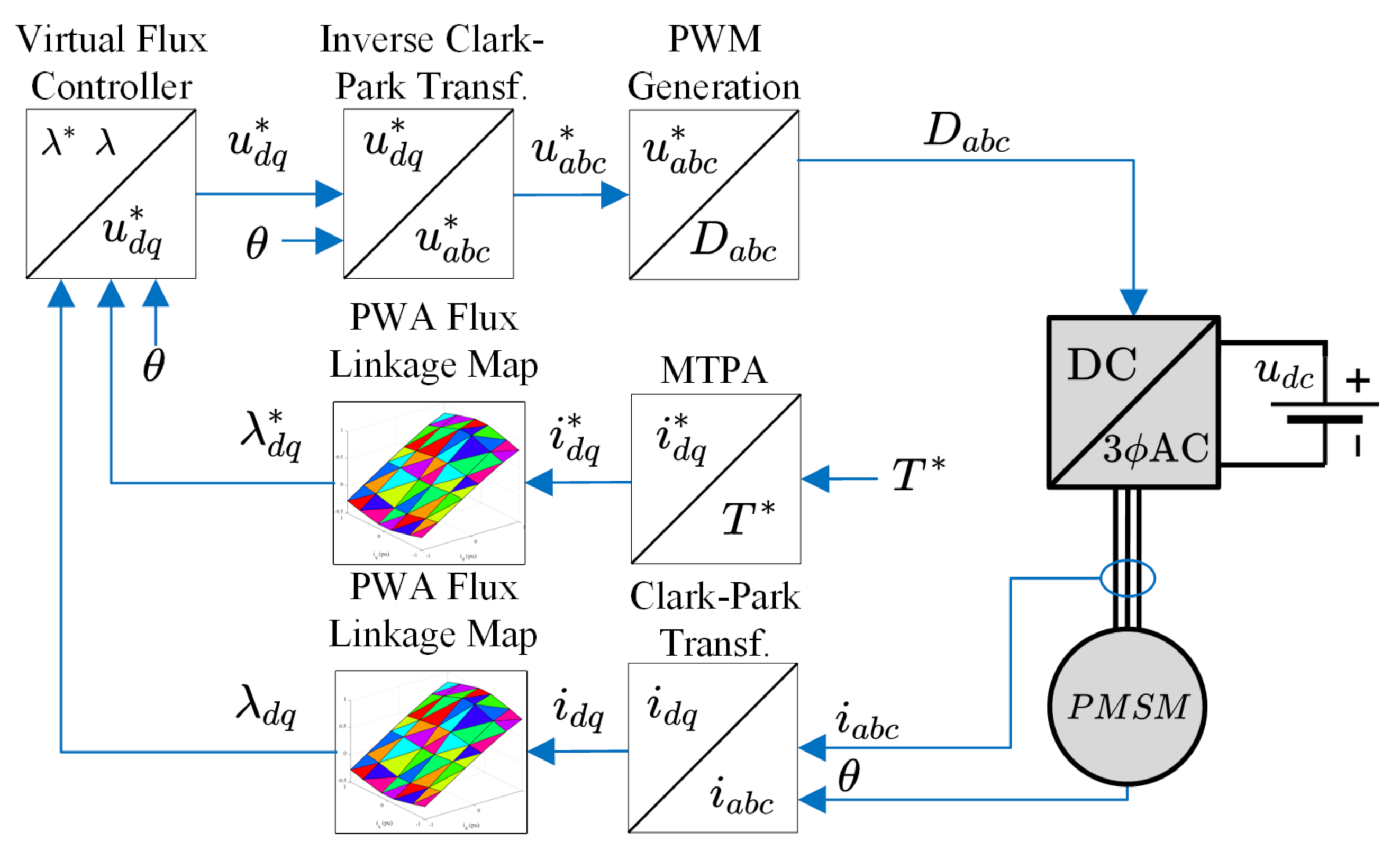
An example motor drive controller set-up is shown in Figure 1, where a three-phase inverter is supplied by $u_{dc}$ and supplies the PMSM with three-phase voltages $u_{ph}$ and currents $i_{ph}$. The input to the controller is a reference torque $T^{*}$, which is translated to a set of reference dq phase currents $i_{dq}^{*}$ by an MTPA function. This reference current $i_{dq}^{*}$ and the fedback and transformed current $i_{dq}$ are independently converted to flux using the $f_{\mathrm{PWA}}$ flux linkage map. The resulting reference flux ${\lambda }_{dq}^{*}$, feedback flux ${\lambda }_{dq}$, and feedback angle $\theta$ go into a virtual flux (VF) controller, such as a VF-MPC. The output is a set of reference dq voltages $u_{dq}^{*}$ which are transformed to phase voltages $u_{abc}^{*}$ and modulated into duty cycles $D_{abc}$ fed to the inverter. This controller demonstrates the order of operations that a DSP can use to implement VF control and the importance of the MM, as it is the only control block used twice in the diagram.

The map $f(·)$ is typically a LUT that is built using measured or Finite Element Analysis (FEA) points that are sampled and interpolated by some method. The map $f(·)$ and torque, created using spline-interpolated FEA datapoints, for a machine with parameters in

Table 2. PMSM motor drive parameters.

Parameter	Value
Type	Interior PM synchronous machine (IPMSM)
Rated current $i_{\mathrm{rated}}$	10 A
Rated torque $T_{\mathrm{rated}}$	8.0 Nm
Rated flux ${\lambda }_{\mathrm{rated}}$	142.5 mWb
Inductance (d-axis) $L_d$	9.1 mH
Inductance (q-axis) $L_q$	14.6 mH
Stator Resistance $R_s$ (@ 20C)	636 m$\Omega$
PM rotor flux $\psi$	88.3 mWb
Pole pair p	5

is shown in Figure 2. The FEA method uses a simulated machine model which includes the machine’s geometry and magnetic properties to approximate the (nonlinear) inductance throughout the machine for a wide range of operating points using the Finite Element Method (FEM). This inductance map is then sampled at high resolution and spline interpolated to create a high fidelity reference MM, $f_S\left(i\right)$ (capital S denoting reference), which is the reference for error calculations in Section 5.

The compensated terminal voltages can be described by the vector $\overline{u}={\left[{\overline{u}}_d{\overline{u}}_q\right]}^{\prime }\in \mathcal{U}$, where $\mathcal{U}$ is the voltage operating range of the machine. Thus, the machine can be described as a standard linear state-space system in the form

$$\begin{array}{cc}\hfill \dot{\lambda }& =\mathbf{A}\lambda +\mathbf{B}\overline{u},\hfill \end{array}$$

(5a)

$$\begin{array}{cc}\hfill i& =g\left(\lambda \right),\hfill \end{array}$$

(5b)

where the $\mathbf{A}$ and $\mathbf{B}$ matrices are

$$\begin{array}{c}\mathbf{A}=\left[\begin{array}{cc}0& \omega \\ -\omega & 0\end{array}\right],\mathbf{B}=\mathbf{I}=\left[\begin{array}{cc}1& 0\\ 0& 1\end{array}\right].\end{array}$$

(6)

The flux $\lambda$ is the state, the compensated voltages $\overline{u}$ are the input, and the current i is the output. This state-space model can be used in an MPC controller. The state $\lambda$ will be linearized using a piecewise affine map $f_{\mathrm{pwa}}\left(i\right)$ according to the machine’s operating point.

3. Piecewise Affine Magnetic Model

This research proposes using a PWA map to represent the PMSM magnetic model. PWA maps take a nonlinear map and divide it into M domains. In each domain, the function is linearized [24]. The PWA current to flux map can be described as

$$\begin{array}{c}\hfill \lambda =f\left(i\right)\approx f_{\mathrm{PWA}}\left(i\right)=\left\{\begin{array}{cc}{\mathbf{L}}_{1}i+{\psi }_1,\hfill & i\in {\mathcal{I}}_1,\hfill \\ {\mathbf{L}}_{2}i+{\psi }_2,\hfill & i\in {\mathcal{I}}_2,\hfill \\ \dots \hfill \\ {\mathbf{L}}_{M}i+{\psi }_M,\hfill & i\in {\mathcal{I}}_M,\hfill \end{array}\right.\end{array}$$

(7)

where $\lambda ={\mathbf{L}}_{j}i+{\psi }_j$ maps the currents $i\in {\mathcal{I}}_j$ onto fluxes $\lambda \in {\Lambda }_j$ as an affine function and the image of the domain ${\mathcal{I}}_j$ is ${\Lambda }_j$. The affine map is defined by a set of equations with a specific inductance matrix ${\mathbf{L}}_j$ and a flux offset vector ${\psi }_j$ for each region.

The inverse of $f(·)$ is

$$\begin{array}{c}\hfill i=g\left(\lambda \right)\approx g_{\mathrm{PWA}}\left(\lambda \right)=\left\{\begin{array}{cc}{\mathbf{L}}_1^{-1}(\lambda -{\psi }_1),\hfill & \lambda \in {\Lambda }_1,\hfill \\ {\mathbf{L}}_2^{-1}(\lambda -{\psi }_2),\hfill & \lambda \in {\Lambda }_2,\hfill \\ \dots \hfill \\ {\mathbf{L}}_M^{-1}(\lambda -{\psi }_M),\hfill & \lambda \in {\Lambda }_M,\hfill \end{array}\right.\end{array}$$

(8)

such that $i=g\circ f\left(i\right)$.

The process to create this PWA MM can be divided into four steps: (1) choose ${\mathcal{I}}_P$, (2) Delaunay triangulation of ${\mathcal{I}}_P$, (3) compute all ${\mathbf{L}}_j$ and ${\psi }_j$ values, and (4) assign all ${\mathbf{L}}_j$ and ${\psi }_j$ values to ${\mathcal{I}}_j$. This process is shown in Figure 3. The following subsections describe each step.

3.1. Choosing ${\mathcal{I}}_P$

${\mathcal{I}}_P\subseteq \mathcal{I}$ is the set of measured [12,13,14,15,17,18,19,20], simulated [12,13,17], or estimated [8,9,10] current points that will be used to create the PWA MM. The corresponding flux set ${\Lambda }_p$ must also be known. In general, there are too many points to all be used to create the MM as, at some point, the PWA function becomes too large for a DSP with finite memory.

${\mathcal{I}}_P$ can be regularly gridded (i.e., $i_d$ and $i_q$ datapoints are evenly separated). The corresponding flux points ${\Lambda }_p$ will not necessarily be regularly gridded. This can be seen in the vertices of the triangles in Figure 4. The particular shape of ${\mathcal{I}}_p$ and ${\Lambda }_p$ will depend on the machine’s operating points or regions. In this case, ${\mathcal{I}}_p$ is bounded by the box constraint ${\mathcal{I}}_p=\{i\in \mathcal{I}|i\le i_{\max }\}$. The shape of the flux image is found using Equation (7) and depends on the inductance throughout the machine. In this case, ${\Lambda }_M$ becomes an irregular shape resembling a bulged rectangle. Other bounds may be a continuous (or derated) current, the MTPA region, etc. These are explored in more detail in Section 5.

An irregularly gridded ${\mathcal{I}}_P$ can yield a higher-accuracy MM for the same number of points as the regularly gridded value because the flux error is not evenly distributed (explored in Section 4). Irregularly gridded current points can also target areas in $\mathcal{I}$ and $\Lambda$ that may be more frequently used, such as derated operation and MTPA. The method for obtaining these sets will be shown in Section 4.

3.2. Subdomains and the Delaunay Triangulation

Building the PWA function requires the domain and image to be split up into M non-overlapping regions or subdomains and subimages, denoted by ${\mathcal{I}}_j$ and ${\Lambda }_j$, respectively. A point $i\in \mathcal{I}$ can only be in two (or more) subdomains if it is on the border $i\in \partial {\mathcal{I}}_j$ of two (or more) subdomains. Points on the borders of two (or more) subdomains guarantee continuity and will also be on the border of the corresponding flux subimages $\lambda \in \partial \Lambda$. Otherwise, points that are not on the border of subdomains are only part of one subdomain and subimage.

The Delaunay triangulation $\mathrm{DT}\left({\mathcal{I}}_P\right)$ [25] of the set of points ${\mathcal{I}}_P$ creates a set of unique, connected simplices ${\mathcal{I}}_M$. The Delaunay triangulation is the dual version of the more familiar Voronoi diagram. The Voronoi diagram of a set of points ${\mathcal{I}}_P\in \mathcal{I}$ splits the space $\mathcal{I}$ into $|{\mathcal{I}}_P|$ “Voronoi cells”, where the points in each cell are closer to some point $i\in {\mathcal{I}}_P$ than any of the other points $i\in {\mathcal{I}}_P$. An example of the Delaunay triangulation in the current and flux space is shown in Figure 5, and a Voronoi diagram in the current domain with the corresponding Delaunay triangulation for an example set ${\mathcal{I}}_P$ is shown in Figure 4.

Each subdomain and subimage is a simplex, which is a triangle in the two dimensions ($dq$) of this problem. (In general, a simplex is the simplest possible polytope given the dimension of the problem.) A simplex can be defined by the convex hull $\mathcal{H}$ of $D+1$ vertices or as a set of $D+1$ affine inequalities (where D is the dimensionality of the problem). These definitions are called V-notation and H-notation, respectively [26]. A simplex in the current domain comprising the vertices $i_{j_0},\dots ,i_{j_D}\in {\mathcal{I}}_P$ is

$$\begin{array}{c}\hfill {\mathcal{I}}_j=\mathcal{H}\left(\{i_{j_0},i_{j_1},\dots ,i_{j_D}\}\right).\end{array}$$

(9)

Each current simplex ${\mathcal{I}}_j$ forms a domain of an affine map that maps onto a flux simplex comprising the vertices ${\lambda }_{j_0},\dots ,{\lambda }_{j_D}\in {\Lambda }_P$, and the flux simplex is

$$\begin{array}{c}\hfill {\Lambda }_j=\mathcal{H}\left(\{{\lambda }_{j_0},{\lambda }_{j_1},\dots ,{\lambda }_{j_D}\}\right).\end{array}$$

(10)

The definition of the Delaunay triangulation (via the Voronoi diagram) implies that the vertices of each simplex are not degenerate (full dimensions) and are linearly independent (in both $\mathcal{I}$ and $\Lambda$ spaces).

3.3. Subdomain Coefficients

As previously explained, a current simplex for the PMSM ${\mathcal{I}}_j$ is defined by $D+1$ (three) vertices as shown in Equaiton (9). A shifted dimension is defined by letting (any) of the vertices $i_{j_0}$ become the new reference origin $\overline{i}=i-i_{j_0}$. The whole simplex thus shifts and becomes

$$\begin{array}{c}\hfill {\overline{\mathcal{I}}}_j=\mathcal{H}(0,{\overline{i}}_{j_1},\dots ,{\overline{i}}_{j_D}\}),\end{array}$$

(11)

where the set of new current vectors ${\overline{i}}_{j_k}=i_{j_k}-i_{j_0}$ spans the simplex. As with the current, we shift the flux space by the corresponding flux vector $\overline{\lambda }=\lambda -{\lambda }_{j_0}$, which results in

$$\begin{array}{c}\hfill {\overline{\Lambda }}_j=\mathcal{H}(0,{\overline{\lambda }}_{j_1},\dots ,{\overline{\lambda }}_{j_D}\}),\end{array}$$

(12)

where ${\overline{\lambda }}_{j_k}={\lambda }_{j_k}-{\lambda }_{j_0}$ spans the simplex and $k=\{1,\dots ,D\}$. The shifted simplices are shown in Figure 6.

The affine map is an isomorphism, and the vertices form the basis, so the position of a vector in the current space relative to the shifted origin is the same as the position of the flux vector from the origin of the shifted flux simplex:

$$\overline{i}=a_1{\overline{i}}_{j_1}+\dots +a_D{\overline{i}}_{j_D}.$$

(13)

The process of computing the a coefficients is similar to computing the relative on times in space vector modulation (SVM) [24]. We start by projecting $\overline{i}$ onto the basis vectors of ${\overline{\mathcal{I}}}_j$:

$$\begin{array}{c}\hfill p_{j_k}={\mathrm{proj}}_{{\overline{i}}_{j_k}}\overline{i}=\frac{{\overline{i}}_{j_k}·\overline{i}}{\parallel {\overline{i}}_{j_k}\parallel },\end{array}$$

(14)

Then, we divide the magnitude of this projection by the magnitude of the shifted basis vectors to obtain the a vector:

$$\begin{array}{c}\hfill a_{j_k}=\frac{\parallel p_{j_k}\parallel }{\parallel {\overline{i}}_{j_k}\parallel }.\end{array}$$

(15)

To calculate the flux, we simply multiply the basis vectors of ${\overline{\Lambda }}_j$ by the a coefficients:

$$\begin{array}{c}\hfill \overline{\lambda }=a_1{\overline{\lambda }}_{j_1}+\dots +a_D{\overline{\lambda }}_{j_D}.\end{array}$$

(16)

Finally, we un-shift the flux to obtain the machine flux at this current point:

$$\lambda =\overline{\lambda }+{\lambda }_{j_0}$$

(17)

Equations (13)–(17) can be compressed using matrix notation. We define the bases of the shifted simplices ${\overline{\mathcal{I}}}_j$ and ${\overline{\Lambda }}_j$ as

$$\begin{array}{cc}\hfill {\mathbf{M}}_{{\overline{\mathcal{I}}}_j}& =\left[{\overline{i}}_{j_1},\dots ,{\overline{i}}_{j_D}\right],\hfill \end{array}$$

(18a)

$$\begin{array}{cc}\hfill {\mathbf{M}}_{{\overline{\Lambda }}_j}& =\left[{\overline{\lambda }}_{j_1},\dots ,{\overline{\lambda }}_{j_D}\right],\hfill \end{array}$$

(18b)

In addition, $a={[a_1,\dots ,a_D]}^T$. Equations (13) and (16) can be rewritten as $\overline{i}={\mathbf{M}}_{{\overline{\mathcal{I}}}_j}a$ and $\overline{\lambda }={\mathbf{M}}_{{\overline{\Lambda }}_j}a$, respectively. Because the simplices are nondegenerate, the bases are nonsingular, and we can find a linear relation:

$$\begin{array}{c}\hfill {\mathbf{M}}_{{\overline{\Lambda }}_j}^{-1}\overline{\lambda }={\mathbf{M}}_{{\overline{\mathcal{I}}}_j}^{-1}\overline{i}.\end{array}$$

(19)

This expression is useful because as long as ${\mathbf{M}}_{{\overline{\Lambda }}_j}$ and ${\mathbf{M}}_{{\overline{\Lambda }}_j}$ exist and are invertible (which they are by the definition of a basis), then the current and flux can be related to each other (in either direction). The flux in terms of the current can be solved by unshifting the basis vectors

$$\begin{array}{c}\hfill {\mathbf{M}}_{{\overline{\Lambda }}_j}^{-1}(\lambda -{\lambda }_{j_0})={\mathbf{M}}_{{\overline{\mathcal{I}}}_j}^{-1}(i-i_{j_0}),\end{array}$$

(20)

and rearranging them to obtain

$$\begin{array}{c}\hfill \lambda ={\mathbf{L}}_{j}i+{\psi }_j,\end{array}$$

(21)

with ${\mathbf{L}}_j={\mathbf{M}}_{{\overline{\Lambda }}_j}{\mathbf{M}}_{{\overline{\mathcal{I}}}_j}^{-1}$ and ${\psi }_j={\lambda }_{j_0}-{\mathbf{L}}_j{i}_{j_0}$. Matrix algebra can be employed to solve for the reverse map $i=g\left(\lambda \right)$ from Equation (8) just as easily.

3.4. Assign Coefficients to Simplices

The coefficients ${\mathbf{L}}_j$ and ${\psi }_j$ are assigned to their simplex ${\mathcal{I}}_j$. Grouping all such functions produces the PWA MM of Equation (7). Examples of differently sized, regularly gridded PWA MM functions are shown in Figure 7.

4. Magnetic Model Optimization

Choosing which areas to minimize the flux error in $f_{\mathrm{PWA}}$ by selectively choosing the points to use ${\mathcal{I}}_P$ depends on the application. The metric chosen to measure the flux error of a PWA MM to the reference (FEA spline) MM at any given point is the 2-Norm flux error. An example of the two-norm flux error distribution using a $13\times 13$ regularly gridded ${\mathcal{I}}_P$ to create $f_{\mathrm{PWA}}$ is shown in Figure 8. The flux error is the highest where the flux linkage is the most nonlinear (see Figure 2).

Given an allotted size for ${\mathcal{I}}_P$, where $|{\mathcal{I}}_P|=N$, an algorithm is devised that chooses ${\mathcal{I}}_P$ to minimize the maximum two-norm flux error. In this algorithm, first, the minimum number of points (${\mathcal{I}}_P$ and ${\Lambda }_P$) to cover the full current domain $\mathcal{I}$ are chosen (step A). In the dq current space, this is a square and thus has four points. Then, steps 2–4 of building $f_{PWA}$ (see Figure 3) are executed (step B). If the size of ${\mathcal{I}}_P$ is less than N, then we compute the two-norm flux error of k random current points in $\mathcal{I}$ (step C). The number k should be much larger than N, where $k\gg N$. Then, we identify the maximum error point ($i_{\max },{\lambda }_{\max }$) (step D). Next, we add the maximum error point to ${\mathcal{I}}_P$ and ${\Lambda }_P$ (step F). This will ensure that the error at this new point in $f_{PWA}$ is $0\%$, and the error surrounding this point will be significantly reduced. Steps B, C, D, E, and F repeat until $|{\mathcal{I}}_P|=N$. The PWA MM algorithm optimization steps (A–F) and PWA MM creation steps (1–4) are shown in Figure 9.

The three areas of interest that will be explored are: the full current range ($\mathcal{I}$), the approximate MTPA trajectory region (${\mathcal{I}}_{\mathrm{MTPA}}$), and the approximate derated current region (${\mathcal{I}}_{\mathrm{derated}}$). $\mathcal{I}$ represents all currents within absolute maximum current limits, $\mathcal{I}=\{i\in \mathcal{I}|i\le i_{\max }\}$. ${\mathcal{I}}_{\mathrm{derated}}$ represents the typical rated or continuous current limit, ${\mathcal{I}}_{\mathrm{derated}}=\{i\in \mathcal{I}|\left|\right|i_{dq}\left|\right|\le i_{\mathrm{rated}}\}$, where in this case $i_{\mathrm{rated}}=0.75pu$. ${\mathcal{I}}_{\mathrm{MTPA}}$ follow the MTPA trajectory [23], and is an area instead of a region to account for temperature variations in the machine parameters. These three regions are shown in Figure 10.

5. Experimental Results

The PWA method of building a MM is evaluated primarily by the flux error. In the following section, $f_{\mathrm{PWA}}$ functions created using irregular optimized grids are evaluated. The points used to construct the model were taken from a large pool of experimental data points, and the flux points were estimated using least squares approximation. For comparison, an $f_{\mathrm{PWA}}$ function using a regularly gridded full current space (${\mathcal{I}}_P=\mathcal{I}$) is used, denoted by ${\mathcal{I}}^{*}$. ${\mathcal{I}}^{*}$ is constructed using square grids (i.e., $2\times 2$, $3\times 3$, ... $6\times 6$), so $N=4,9,...36$. All data for this section came from an IPMSM with the parameters shown in Table 2. The magnetic model was compared against a high-fidelity, spline-interpolated MM built using many FEA data points, denoted by $f_S$.

Flux Error Analysis

The flux error in an MM will propagate to an error in the state-space model of the system from Equation (5) and the torque from Equation (2). The two-norm flux error between $f_{\mathrm{PWA}}$ using the irregular optimization algorithm of Section 4 and $f_S$ (high-fidelity model) can be evaluated by sampling many random current points $i\in \mathcal{I}$. The average and maximum of this error within the optimized regions for various values of N are shown in Figure 11. The linear inductance magnetic model ($\mathbf{L}$ and $\psi$ constant throughout all of $\mathcal{I}$) are also shown, as well as a spline-interpolated magnetic model (lowercase ‘s’, indicating it is not a high-fidelity model) $f_s$ focusing on the MTPA region. Among the irregular optimized PWA functions, the error was the smallest for the MTPA region as this was the smallest region by area, and the error was the largest for $\mathcal{I}$ as this was the largest area. It can be seen that the average and maximum errors of ${\mathcal{I}}^{*}$ (regularly gridded) were significantly worse by margins of $\approx 1–3\%$ and $\approx 5–8\%$ respectively.

As expected, the linear MM $f_l\left(i\right)$ had a much higher flux error than the PWA models by $\approx 20–30\%$ on average and $\approx 25–40\%$ maximum. The spline interpolated MM focusing on the MTPA region outperformed the PWA MM by $\approx 1–3\%$ for the average error and $\approx 1–6\%$ for the maximum error. The decreased error is beneficial but does not allow for the linear state-space model (Equation (5)).

The error distribution in these MMs was not even. As an example, the functions using 36-point ($6\times 6$) regularly gridded current points (${\mathcal{I}}^{*}$) and 40-point irregularly gridded functions ($\mathcal{I}$, ${\mathcal{I}}_{\mathrm{MTPA}}$, and ${\mathcal{I}}_{\mathrm{derated}}$) are shown in Figure 12. The simplical mesh ${\mathcal{I}}_M$ composed of all simplices ${\mathcal{I}}_j$ is shown in the top row, the placement of points in ${\mathcal{I}}_P$ by the optimization algorithm for each of these functions is shown in the middle row, and the two-norm flux error distribution is shown in the bottom row. The two-norm flux error was minimized only in the region of interest, which is apparent in the low flux error, especially for ${\mathcal{I}}_{MTPA}$ and ${\mathcal{I}}_{derated}$.

6. Conclusions

In this study, a formal method for creating piecewise affine flux linkage maps for a PMSM is presented using a four-step process. This model is linear while also capturing saturation, a useful combination for efficient and robust VF-MPC control. A six-step process for optimizing the magnetic model for a given region is also shown, and the optimization is presented for the MTPA and derated regions of operation. Experimental data points were compared to the FEA-simulated datapoints for a wide range of model resolutions, with an average flux error of less than $1\%$ and a maximum error of less than $3\%$ when using only 40 points. Over the full range of model resolutions, there was a $\approx 1–3\%$ and $\approx 5–8\%$ reduction in the flux error compared with a regularly gridded model.

References

1. Bilgin, B.; Magne, P.; Malysz, P.; Yang, Y.; Pantelic, V.; Preindl, M.; Korobkine, A.; Jiang, W.; Lawford, M.; Emadi, A. Making the Case for Electrified Transportation. IEEE Trans. Transp. Electrif. 2015, 1, 4–17. [Google Scholar] [CrossRef]
2. Dai, Y.; Song, L.; Cui, S. Development of PMSM Drives for Hybrid Electric Car Applications. IEEE Trans. Magn. 2007, 43, 434–437. [Google Scholar] [CrossRef]
3. Brelje, B.J.; Martins, J.R. Electric, hybrid, and turboelectric fixed-wing aircraft: A review of concepts, models, and design approaches. Prog. Aerosp. Sci. 2019, 104, 1–19. [Google Scholar] [CrossRef]
4. Sayed, E.; Abdalmagid, M.; Pietrini, G.; Sa’adeh, N.M.; Callegaro, A.D.; Goldstein, C.; Emadi, A. Review of Electric Machines in More-/Hybrid-/Turbo-Electric Aircraft. IEEE Trans. Transp. Electrif. 2021, 7, 2976–3005. [Google Scholar] [CrossRef]
5. Fernandez, D.; Hyun, D.; Park, Y.; Reigosa, D.D.; Lee, S.B.; Lee, D.M.; Briz, F. Permanent Magnet Temperature Estimation in PM Synchronous Motors Using Low-Cost Hall Effect Sensors. IEEE Trans. Ind. Appl. 2017, 53, 4515–4525. [Google Scholar] [CrossRef] [Green Version]
6. Kang, G.H.; Hur, J.; Nam, H.; Hong, J.P.; Kim, G.T. Analysis of irreversible magnet demagnetization in line-start motors based on the finite-element method. IEEE Trans. Magn. 2003, 39, 1488–1491. [Google Scholar] [CrossRef]
7. Fernández, D.; Martínez, M.; Reigosa, D.; Guerrero, J.M.; Suárez Alvarez, C.M.; Briz, F. Impact of Machine Magnetization State on Permanent Magnet Losses in Permanent Magnet Synchronous Machines. IEEE Trans. Ind. Appl. 2019, 55, 344–353. [Google Scholar] [CrossRef]
8. Alessandri, A.; Baglietto, M.; Battistelli, G. Receding-horizon estimation for switching discrete-time linear systems. IEEE Trans. Autom. Control 2005, 50, 1736–1748. [Google Scholar] [CrossRef]
9. Brosch, A.; Hanke, S.; Wallscheid, O.; Böcker, J. Data-Driven Recursive Least Squares Estimation for Model Predictive Current Control of Permanent Magnet Synchronous Motors. IEEE Trans. Power Electron. 2021, 36, 2179–2190. [Google Scholar] [CrossRef]
10. Wlas, M.; Krzeminski, Z.; Toliyat, H.A. Neural-Network-Based Parameter Estimations of Induction Motors. IEEE Trans. Ind. Electron. 2008, 55, 1783–1794. [Google Scholar] [CrossRef]
11. Li, X.; Kennel, R. General Formulation of Kalman-Filter-Based Online Parameter Identification Methods for VSI-Fed PMSM. IEEE Trans. Ind. Electron. 2021, 68, 2856–2864. [Google Scholar] [CrossRef]
12. Chen, H.; Yan, W.; Wang, Q. Electromagnetic Analysis of Flux Characteristics of Double-Sided Switched Reluctance Linear Machine. IEEE Trans. Appl. Supercond. 2016, 26, 1–7. [Google Scholar] [CrossRef]
13. Liu, K.; Feng, J.; Guo, S.; Xiao, L.; Zhu, Z.Q. Identification of Flux Linkage Map of Permanent Magnet Synchronous Machines Under Uncertain Circuit Resistance and Inverter Nonlinearity. IEEE Trans. Industr. Inform. 2018, 14, 556–568. [Google Scholar] [CrossRef]
14. Bedetti, N.; Calligaro, S.; Petrella, R. Stand-Still Self-Identification of Flux Characteristics for Synchronous Reluctance Machines Using Novel Saturation Approximating Function and Multiple Linear Regression. IEEE Trans. Ind. Appl. 2016, 52, 3083–3092. [Google Scholar] [CrossRef]
15. Armando, E.; Guglielmi, P.; Pellegrino, G.; Bojoi, R. Flux linkage maps identification of synchronous AC motors under controlled thermal conditions. In Proceedings of the 2017 IEEE International Electric Machines and Drives Conference (IEMDC), Miami, FL, USA, 21–24 May 2017; pp. 1–8. [Google Scholar]
16. Ichikawa, S.; Tomita, M.; Doki, S.; Okuma, S. Sensorless control of permanent-magnet synchronous motors using online parameter identification based on system identification theory. IEEE Trans. Ind. Electron. 2006, 53, 363–372. [Google Scholar] [CrossRef]
17. Wang, Q.; Zhang, G.; Wang, G.; Li, C.; Xu, D. Offline Parameter Self-Learning Method for General-Purpose PMSM Drives with Estimation Error Compensation. IEEE Trans. Power Electron. 2019, 34, 11103–11115. [Google Scholar] [CrossRef]
18. Armando, E.; Bojoi, R.I.; Guglielmi, P.; Pellegrino, G.; Pastorelli, M. Experimental Identification of the Magnetic Model of Synchronous Machines. IEEE Trans. Ind. Appl. 2013, 49, 2116–2125. [Google Scholar] [CrossRef] [Green Version]
19. Seilmeier, M.; Piepenbreier, B. Identification of steady-state inductances of PMSM using polynomial representations of the flux surfaces. In Proceedings of the IECON 2013—39th Annual Conference of the IEEE Industrial Electronics Society, Vienna, Austria, 10–13 November 2013; pp. 2899–2904, ISSN 1553-572X. [Google Scholar]
20. Chen, H.; Sun, C.; Wang, Q. Analysis of Flux-Linkage Characteristics of Switched Reluctance Linear Generator. IEEE Trans. Appl. Supercond. 2014, 24, 1–5. [Google Scholar] [CrossRef]
21. Steyaert, B.; Swint, E.; Pennington, W.W.; Preindl, M. Piecewise Affine Modelling of Wound-Rotor Synchronous Machines for Real-Time Motor Control. IEEE Trans. Ind. Electron. 2022, 1–10. [Google Scholar] [CrossRef]
22. Preindl, M. Robust Control Invariant Sets and Lyapunov-Based MPC for IPM Synchronous Motor Drives. IEEE Trans. Ind. Electron. 2016, 63, 3925–3933. [Google Scholar] [CrossRef]
23. Preindl, M.; Bolognani, S. Optimal State Reference Computation With Constrained MTPA Criterion for PM Motor Drives. IEEE Trans. Power Electron. 2015, 30, 4524–4535. [Google Scholar] [CrossRef]
24. Samuel, P.; Levy, S. Projective Geometry; Undergraduate Texts in Mathematics; Springer: New York, NY, USA, 1988. [Google Scholar]
25. Aurenhammer, F. Voronoi Diagrams, a Survey of a Fundamental Geometric Data Structure. ACM Comput. Surv. 1991, 23, 345–405. [Google Scholar] [CrossRef]
26. Borrelli, F.; Bemporad, A.; Morari, M. Predictive Control for Linear and Hybrid Systems; Cambridge University Press: Cambridge, UK, 2017. [Google Scholar]
Figure 1. Example motor drive system (gray) and virtual flux controller architecture (white) demonstrating the use of the PWA MM flux linkage map.
Energies 15 07259 g001
Figure 2. (top) (left) The d-axis flux linkage map, (middle) q-axis flux linkage map, and (right) torque function. (bottom) (left) The d-axis iso-flux lines, (middle) q-axis iso-flux lines, and (right) iso-torque lines.
Energies 15 07259 g002
Figure 3. Four-step process to create a piecewise affine (PWA) magnetic model (MM).
Energies 15 07259 g003
Figure 4. (left) Mesh of simplices I j I M created using a 13-by-13 regularly gridded I P in current space. (right) Corresponding mesh of simplices Λ j Λ M in flux space.
Energies 15 07259 g004
Figure 5. Voronoi diagram (left) of a seven-point irregular current grid and the corresponding eight-simplex Delaunay triangulation (right).
Energies 15 07259 g005
Figure 6. Visualization of f pwa : (left) current simplex (triangle) I j ¯ shifted by i j 0 vector and (right) corresponding flux simplex (triangle) Λ ¯ j shifted by λ j 0 vector.
Energies 15 07259 g006
Figure 7. PWA MM functions at various resolutions using regularly gridded I P : (left) d-axis flux λ d from f PWA and (right) q-axis flux λ d .
Energies 15 07259 g007
Figure 8. Two-norm flux error distribution between f PWA ( i ) and f S ( i ) , f PWA ( i ) constructed using regularly gridded 13 × 13 I P , where f S ( i ) uses high-fidelity spline-interpolated FEA data points.
Energies 15 07259 g008
Figure 9. PWA MM optimization algorithm to minimize the maximum two-norm flux error in f PWA given an allotted N number of of points to use ( | I P | = N ).
Energies 15 07259 g009
Figure 10. Visualization of three regions of current to optimize f PWA : I , I MTPA , and I derated .
Energies 15 07259 g010
Figure 11. (left) Average and (right) maximum two-norm flux error vs. N points in various magnetic models (MMs): PWA f PWA ( i ) (targeting error reduction in specific regions), linearized inductance model f l ( i ) , and spline model f s ( i ) (targeting error reduction in MTPA region).
Energies 15 07259 g011
Figure 12. (top row) Simplical mesh I M comprising all simplices I j . (middle row) Placement of points in I P by the optimization algorithm. (bottom row) Two-norm flux error distribution. (first column) f PWA using regularly gridded current points covering I . (second column) f PWA using irregularly gridded current points optimizing I . (third column) f PWA using irregularly gridded current points optimizing I MTPA . (fourth column) f PWA using irregularly gridded current points optimizing I derated .
Energies 15 07259 g012