Abstract
Wear debris in lubrication oil provides important information for marine engine condition monitoring and faults diagnosis. Inductive sensors have been widely used to detect wear debris in lubrication oil. To improve the sensitivity, the inductive coil is always connected with a capacitor in parallel to form parallel LC resonance-sensing circuit. A previous study optimized the parallel resonance circuit by adjusting the excitation frequency. However, multiple parameters (namely, excitation signal, signal detection circuits, and signal-processing program, etc.) need to be adjusted accordingly for a series of the testing frequencies. To simplify the optimization, we propose a method based on adjusting the parallel capacitance in this work. The impedance (inductance and internal resistance) of the sensing coil and its variation induced by particles are first measured, which are the necessary parameters for establishing the function relationship between the parallel capacitance and the relative impedance variation. With the function relationship, the relative impedance variation is calculated directly, and the optimal capacitance is located at the highest absolute value of it. The experimental results for the ferrous and nonferrous particles match the calculation results well. Interestingly, the optimal capacitance for the nonferrous particle was larger than that of the ferrous particle. We speculate that the difference is generated due to the increased resistance induced by the eddy current effect.
1. Introduction
Frequent machine health condition and failure analysis is vital to ensure continuous performance and safety of marine engines. Accurate real-time assessment of the engine status can help avoid lapses in operation by emergency shutdowns, major maintenance works, and catastrophic accidents, significantly saving cost and resources. Methods, such as vibration analysis, infrared thermography, ultrasound, acoustic emissions, etc., are commonly and regularly employed in this regard [1,2,3,4,5]. However, the detection of possible faults with these methods often involves complex data acquisition and assessment steps. Wear contaminants in the lubricating oils of these machineries also convey valuable information about the health [6,7,8]. In addition, this method of evaluating the engine conditions by analyzing the lubricant oil for the wear debris has also found strong interest lately for aircraft engines, wind turbines, and hydraulic equipment [9,10].
Owing to the ability to differentiate ferrous and nonferrous metal particles, inductive sensors have been widely used for real-time online wear debris detection [11,12,13]. When the sensing coil is excited by sine wave signal, the particle passing through the sensing coil causes impedance change by the magnetization effect and the eddy current effect. This in turn leads to the voltage change of the output signal. Many studies have been conducted over the decades in this area to have better detection sensitivity. The inductive sensor detection system can be separated into different units, such as excitation signal, inductive sensor, signal detection circuit, and signal post processing program. The optimization works can be done on these units to improve the final detection signal. For example, higher excitation voltage can generate strong magnetic field in the sensing area, benefiting the signal detection [14]; high excitation frequency can induce a strong eddy current effect, resulting in enhanced impedance change of the sensor for nonferrous particle [15,16]; two double-wire solenoid coils can improve detection sensitivity [17]; small inner diameter of the sensing coil and special sensor structure can lead to high magnetic flux density [18,19,20,21]; ferrite cores and other high permeability materials can further enhance the magnetic flux density in the sensing coil [21,22,23,24,25,26,27]; the external circuit of the sensing coil [28] and the signal post processing program [29,30,31,32] also help produce a high-quality detection signal.
The inductive sensors are also generally connected to a capacitor in parallel to form a parallel inductance–capacitance (LC) resonance circuit [33,34], which facilitates increased sensitivity. Du et al. first proposed the parallel resonance circuit for wear debris detection [35]. Ren et al. and Wu et al. further proved its effectiveness in application [36,37,38]. Du et al. performed optimization of the parallel resonance circuit to obtain a better output signal [14]. They applied a series of sine waves with different frequencies to the parallel resonance circuit to find the optimal frequency at which the magnitude of the output signal was largest. They found that the optimal frequency for ferrous particles was different from that for nonferrous particles.
In this work, we aimed to optimize the parallel resonance circuit by adjusting the parallel capacitance, . The capacitor is straightforward to be replaced and does not need any additional adjustments to the sensing system. A sine wave of 2 MHz frequency is adopted as the excitation signal since this high frequency would ensure enhanced eddy current effect, thus benefiting the nonferrous particle detection. The relative impedance variation of the LC resonance circuit is used as the metric to evaluate the detection quality. We also theoretically calculate the relative impedance variation induced by the ferrous and the nonferrous particles used. Then, verifications are made with the experimental results for both the ferrous and nonferrous particles for a range of parallel capacitances (from 0.0 nF to 3.0 nF).
2. Determination of the Optimal Capacitance
2.1. The Impedance Variation in the Sensing Coil
The impedance of the sensing coil is mainly influenced by the magnetization effect and the eddy current effect by metal particles [39,40,41,42]. For ferrous particles, the magnetization effect is relatively much stronger than the eddy current effect [19,28]. The significantly higher magnetic permeability, , of the ferrous particles lead to an increase in the inductance causing the change in impedance. For nonferrous metal particles, the magnetization effect is absent and only the eddy current effect is generated by the particle. However, the eddy current not only induces the inductance decrease but also leads to increased resistance. The eddy current effect of the particle on the sensing coil can be illustrated with a principle similar to that of an alternating current (AC) transformer, as shown in Figure 1a. Here, the sensing coil is modeled as the primary side of the transformer with an input voltage, , inductance, L1, and internal resistance, R1. The particle is modeled as the secondary side containing the inductance, L2, and the internal resistance, R2, but no load. is the mutual inductance between the sensing coil and the particle. The voltage equations for the sensing coil and the particle can be expressed as
where ω = 2 πf is the angular velocity. If we express the eddy current effect that acts on the sensing coil as ΔZeq, as shown in Figure 1b, and the input sine wave voltage as , from Equation (1) we can get
where is the real part and is the imaginary part of . Thus, evidently, the eddy current will not only induce the decrease in inductance but also lead to the increase of resistance.
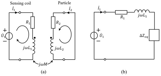
Figure 1.
Illustration of the eddy current effect induced in the particle by the sensing coil with (a) separate circuit model and (b) an equivalent circuit.
The above analysis only provides a qualitative understanding of the eddy current effect on circuit impedance. However, the particle size and material are important factors for the eddy current effect. The larger the size, the larger the induced electromotive force inside the metallic particle. With the same size, the induced electromotive forces are the same. However, higher conductivity of the particle will induce a higher eddy current. As shown in Table 1, five spherical iron particles and five spherical copper particles with different sizes (referencing the actual wear debris size) will be tested in our experiment. The conductivity of the iron particle is S/m, and the conductivity of the copper particle is S/m. The copper particle will induce a higher eddy current inside the particle with the same size as the iron particle. Iron and copper particles are represented for ferrous and nonferrous particles, respectively.

Table 1.
The impedance variation induced by iron and copper particles.
To further support the analysis above, we experimentally tested the impedance of five iron particles and five copper particles. Ten particles were tested five times with an Agilent E4980A Precision LCR meter to obtain the average impedance variations (ΔR and/or ΔL). Parts of the impedance variation induced by iron and copper particles are shown in Figure 2. As we can see, the copper particle can induce obvious resistance variation. However, there is almost no resistance variation in iron particles. With similar size, the 188 μm iron particle induces the resistance variation of 0.00222 Ω, but the 182 μm copper particle induces the resistance variation of 0.02624 Ω. Thus, the eddy current effect is much stronger in the copper particle than the iron particle.
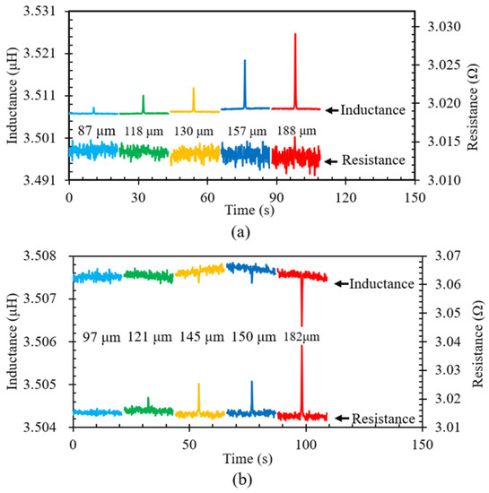
Figure 2.
The inductance and resistance variations of the sensing coil induced by (a) iron and (b) copper particles measured by LCR meter.
Table 1 shows the average impedance variation of ten particles. The 97 μm copper particle is too small to see the inductance and resistance variation. The measured impedance variations from here were then used to calculate the relative impedance variation of the parallel LC resonance circuit. The sensing coil used has 50 turns, an inner diameter of 1 mm, an outer diameter of 2 mm, axial length of 380 μm, and a wire diameter of 65 μm. The inductance of the sensing coil is 3.507 μH, and the resistance is 3.015 Ω. Even though the LCR meter is able to measure the impedance variation, it is not sensitive enough to detect small particles, and the LCR meter is not able to detect metal particles at high speed which would highly limit the oil wear debris detection throughput.
2.2. Relative Impedance Variation of Parallel LC Resonance Circuit
Figure 3 shows the equivalent parallel inductance–capacitance (LC) resonance circuit. The inductive sensing coil is modeled as an inductance, , in series with resistance, . The capacitor, , is connected to the sensing coil in parallel forming the parallel LC resonance circuit. The impedance could be expressed as
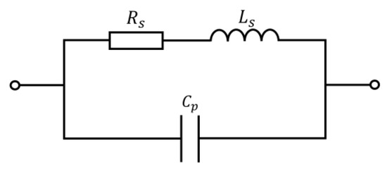
Figure 3.
The parallel inductance–capacitance resonance circuit where, = 3.015 Ω, = 3.507 μH, and ranged from 0 nF to 3.0 nF.
As mentioned earlier, we optimized the parallel resonance circuit by adjusting its capacitance, . Hence, the absolute value of impedance, , was also calculated as a function of , shown (the dash-dotted line in black) in Figure 4.
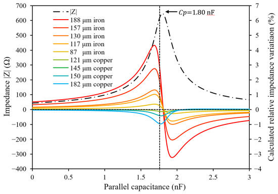
Figure 4.
The calculated absolute value of impedance, , for the coil circuit (dashed black line, left axis) and the relative impedance variations for the iron and copper particles for the range of with the excitation frequency of 2 MHz (right axis).
Since , the resonance frequency is approximately . Here, reached the maximum at the resonance capacitance of 1.80 nF with the excitation frequency of 2 MHz.
We use the relative impedance variation as the metric to evaluate the parallel resonance circuit. The same particle would induce different relative impedance variations with different parallel capacitances. Hence, the highest absolute value of the impedance variation corresponds to the optimal parallel capacitance for the system. The relative impedance variation could be expressed as
where is the impedance of the parallel resonance circuit when the particle passes through the sensing coil.
2.3. Estimation of the Optimal Capacitance
To estimate the optimal capacitance of the parallel resonance circuit, we checked the relative impedance variation for capacitances between 0.0 nF and 3.0 nF. The influence of parasitic capacitance on the system was ignored as the overall performance of the coil was also inductive. Figure 4 shows the relative impedance variations calculated with the measured inductance change, , and resistance change, , for five iron particles and four copper particles. The calculated results for iron particles for the range of capacitances followed a sine wave-like pattern, gradually reaching a positive peak and then falling to a negative peak before getting back close to null. However, the absolute value of the positive peak was a little larger than that of the absolute negative peak. For 188 μm iron particle, the positive peak (4.3229%) is larger than the negative peak (3.2324%). For the copper particle on the other hand, the calculated relative impedance variation did not follow the ideal sine wave-like pattern anymore. It was shifted towards the negative direction with first a negative peak occurring with a large absolute magnitude, then rising above zero, and abruptly increasing immediately afterwards to reach a positive peak; it decreased slowly hereafter but stayed on the positive side until the highest tested capacitance. For the 182 μm copper particle, the absolute negative peak (0.9659%) was almost 23.5 times greater than the highest absolute positive value occurring at the end (0.04102%). We speculate that this difference of the trends between ferrous (iron) and nonferrous (copper) particles was because of the resistance increase due to the eddy current effect of nonferrous particles. The increase in resistance being absent, the decrease of inductance only would cause the relative impedance variation for the nonferrous particles to follow an inverted sine wave-like shape.
The optimal capacitance by definition was located at the maximum absolute value of the relative impedance variation. The optimal capacitances for the detection of iron and copper particles with different diameters can be obtained from Figure 4. As shown in Figure 5, the optimal capacitances of two kinds of particles both decrease a little with the increase of diameter. For iron particles, the optimal capacitance decreases from 1.690 nF to 1.685 nF with the diameter increase from 87 μm to 188 μm, and the variation is 0.005 nF. For copper particles, the optimal capacitance decreases from 1.806 nF to 1.772 nF with the diameter increase from 121 μm to 182 μm, and the variation is 0.034 nF. The variation of copper particles is higher than iron particles. Furthermore, the optimal capacitances between iron and copper particles are obviously different. Even through the difference between two optimal capacitances is not large, it cannot be neglected because the relative impedance variations are highly sensitive to small capacitance changes near the optimal capacitances.
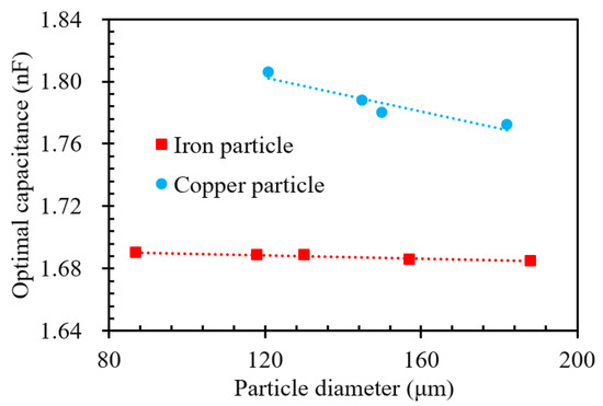
Figure 5.
The optimal capacitance for the detection of different sizes of iron and copper particles.
3. Experiment Method and Setup
3.1. Signal Detection Method
The relative impedance variations were measured by a signal detection system organized, as illustrated in Figure 6. The sensing coil is modeled as an inductance, Ls, in series with a resistance, Rs. A capacitor, Cp, is connected to the sensing coil in parallel to form a parallel resonance circuit, highlighted in the red-dotted frame. The sine wave excitation signal was produced by the function generator and was applied to the sensing coil by the gain inverting amplifier circuit. The output signal, Vout, is proportional to the impedance, Z, of the parallel circuit, which can be expressed by
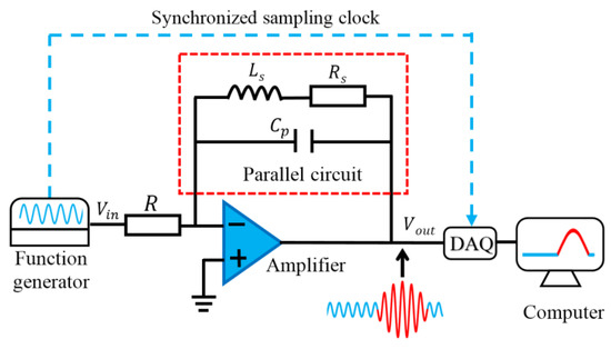
Figure 6.
The schematic diagram of the experimental setup for the signal detection with the parallel LC resonance circuit.
Thus, the relative impedance variation, Δ|Z|/|Z|, could be calculated by dividing the voltage variation, ΔV, with the voltage baseline, V. The output signal was detected with data acquisition equipment (DAQ) using the synchronized sampling method [36,43]. The peak value of the sine wave signal can be recorded with this method. The particle that passes through the sensing coil induces an impedance change in the parallel resonance circuit that further reflects on the amplitude of the output signal, as the red signal shown in Vout. Finally, a pulse would appear in the voltage variation curve sampled by the DAQ.
3.2. Particle Preparation
To mimic the wear particle detection by the inductive sensing coil, a single particle is placed on a nylon fiber, as shown in Figure 7. The nylon fiber is first wetted with usual glue, then the particle was attached onto the viscous fiber surface, as illustrated in Figure 7b. The glue is then dried out in the air for a long enough time to ensure the particle’s attachment. Then, the fixed particle is dipped into the glue again to surround the particle completely (as shown in Figure 7c) to avoid any risk of the particle falling off the fiber. It should be noted that the glue and nylon wire will not induce the change of inductance which has previously been experimentally verified. The particles used in the experiment were almost spherical; thus, the size could be estimated by directly measuring the diameter under the microscope. To investigate the capacitance effect, we tested five iron particles and five copper particles, as declared in Table 1. For the sensitivity test of the system with the optimal capacitances, a range of iron particles with sizes from 22 μm to 188 μm and copper particles with sizes from 62 μm to 182 μm were checked.
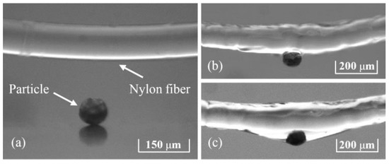
Figure 7.
The attachment procedure of the particle to be tested on a nylon fiber, (a) the 89 μm metal particle and the 115 μm in diameter nylon fiber; (b) the initial attachment of the particle on the fiber by glue; and (c) the finally attached particle completely surrounded by the glue.
3.3. Setup and Testing
Figure 8a shows the actual image of the experimental setup with which the tests were conducted. Single particles that were fixed on the nylon fibers were driven by a step motor through the center of the sensing coil repeatedly. Two terminals of the nylon fiber were bonded on two slide stages which were driven by the step motor. In this experiment, the axial length of the coil is 380 μm. The inner diameter is 1.0 mm, the outer diameter is 2.1 mm, and the wire diameter is 65 μm (including insulating paint, the diameter of the metal part is 50 μm), the number of turns is 50. The coil inductance is 3.507 μH. A glass tube was placed in the center of the sensing coil for the nylon fiber with the particle to pass through. It had a length of 12 cm and an inner diameter of 500 μm which restricted the radial movement of the particles, thus reducing the effect of magnetic flux density generated by the lateral movements in the sensing process. The glass tube was held at the center of the coil with a three-axis precision moving stage. The sensing coil was fabricated with an automatic hot air winder. The step motor was operated by a controller to pass the particle through the sensing coil back and forth repeatedly with a speed of 5.1 cm/s. Since the particle passes through the sensing coil again and again, several pulses are seen in the recorded voltage variation curve. Figure 8b shows the detection signal when an 86 μm iron particle reciprocally (repeatedly back and forth) passes through the sensing coil with the parallel capacitance of 1.60 nF. Two adjacent pluses here are the induced pulses by the particles moving in opposite directions.
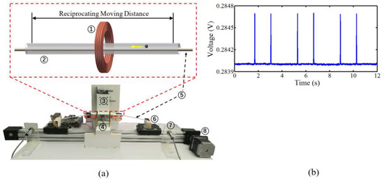
Figure 8.
(a) The experimental setup with (1) sensing coil, (2) glass tube, (3) three-axis precision moving stage, (4) signal detection circuit, (5) nylon fiber, (6) slide stages, (7) electromagnetic limit switches, and (8) step motor. (b) The detection signal when an 86 μm iron particle reciprocally passes through the sensing coil.
This measurement setup has two advantages: (1) the particle is fixed on the nylon fiber which makes it possible to repeatedly conduct the signal detection by the same particle, and (2) the nylon fiber is tightly bonded with the two slide stages to ensure that the particle keeps the same speed with the slide stage. The constant speed of the slide stage helped avoid the speed influence.
The sine wave excitation signal was produced by a function generator (National Instruments PXI-5422 arbitrary waveform generator). The output signal was recorded with a DAQ (National instruments PXIe-6124 multifunction I/O module) using the synchronized sampling method. The synchronization signal from the function generator works as the sampling clock for the DAQ. The parallel capacitors (ceramic, muRata) that were used in the circuit ranged from 10 pF to 3.0 nF with the error tolerance of ±10 pF. Two capacitors were combined in parallel if needed to have a cumulative capacitance that cannot be found by a single capacitor. In the experiment, ten particles were first detected with same capacitor so that the signals of the particles under this capacitance are comparable. After that, these particles were detected with different capacitances. Because of the capacitance error, the new capacitor may be of different capacitances. The excitation voltage signal for the parallel circuit was kept constant (0.56 Vpp, 2 MHz), then the input signal, Vin, and the resistance, R, in the inverting amplifier were adjusted along with the parallel capacitance.
4. Results and Discussion
4.1. Verification of Optimal Capacitance for Ferrous Particle
To verify the estimated optimal capacitance in Section 2.3, the five iron particles were firstly tested with the parallel capacitances from 0.0 nF to 3.0 nF. The recorded voltages of the output signal, Vout, as the particle passed through the coil was then used to calculate the relative impedance variations. Figure 9 shows the relative impedance variations with the error bars for each parallel capacitance. The experimental results matched well with the theoretically calculated results. The curves for the five iron particles followed a similar sine wave-like shape here as well. For the 188 μm iron particle, the relative impedance variation increased from 0.3086% (0 nF) to a peak of 3.8890% (1.69 nF) and then steeply decreased to 0% (1.82 nF). Hence, the magnitude of the relative impedance variation could be increased by 12.6 times. It further decreased with the increase of capacitance to reach a minimum point of −2.8818% (2.00 nF). After this point, it gradually increases again but stays negative until 3.0 nF. At the same time, it should be noted that there were differences between the experimental results and the calculated results. These differences may be due to the errors during impedance variation measuring and experimental detection.
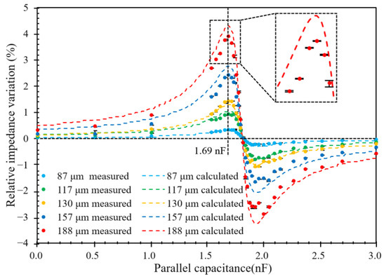
Figure 9.
The relative impedance variation induced by iron particles for different capacitances.
The trend for the relative impedance variation here could be explained with the help of Figure 10. The relative impedance variation is basically generated from the difference between the impedance with ferrous particle, |Z’|, and without the particle, |Z|. Comparing with the curve of |Z|, the curve of |Z’| seems to be improved and moved to the left by the magnetization effect. The impedance difference, (|Z’| − |Z|), increases with the capacitance at the beginning. It reaches the maximum point and then decreases to zero at the cross point of |Z’| and |Z|. After the zero point, |Z’| is smaller than |Z|, and thus, the difference becomes negative.
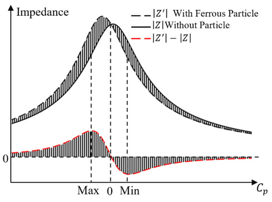
Figure 10.
Schematic of impedance development with and without the ferrous particles passing through the coil and the calculated impedance difference.
The absolute value of the maximum point was larger than the absolute value of the minimum point, and the optimal parallel capacitance was located to be at the maximum point. In Figure 9, the optimal capacitances of five iron particles are all located at 1.69 nF. Thus, the calculated results could reliably be used to estimate the optimal capacitance for the ferrous particle.
4.2. Verification of Optimal Capacitance for Nonferrous Particle
Figure 11 shows the measured relative impedance variations with error bars for the test run with five copper particles. The experimental results again show good agreement with the calculated result. For the 182 μm copper particle, the relative impedance variation first grew in the negative direction, decreasing from −0.03945% (1.01 nF) to a minimum of −1.01739 (1.78 nF), after which point it increased with the increment of capacitance. It reached 0% (2.05 nF) quickly from the minimum point and reached a maximum point of 0.07153% (2.52 nF). After the maximum point, the relative impedance variation decreased slowly but stayed in the positive side as 3.0 nF.
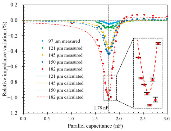
Figure 11.
The relative impedance variations induced by five copper particles for different capacitances.
The growth trend of the nonferrous particle is opposite of the ferrous particle, as can be seen in Figure 12. Compared to the impedance, |Z|, the impedance as the nonferrous particle passes through, |Z’|, was reduced and shifted to the right due to the eddy current effect. As a result, the impedance difference, (|Z’| − |Z|), is negative on the left side of the cross point of |Z| and |Z’| and positive rightwards of it. The highest absolute value of the relative impedance variations for 182 μm, 150 μm, and 145 μm copper particles occurs at 1.78 nF. However, the optimal capacitances for the 97 μm and 121 μm copper particles are not able to be found for the unstable data near the peak, which may result from the small particle size and the setup detection accuracy limitation. Thus, the optimal capacitance is located at 1.78 nF, which is within the calculated optimal capacitance range.
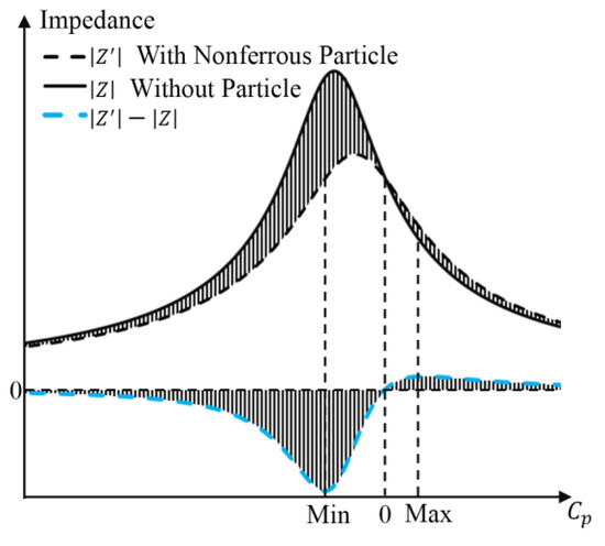
Figure 12.
Schematic of impedance development with and without the nonferrous particles passing through the coil and the calculated impedance difference.
The growth trends of the relative impedance variations show that the ferrous and nonferrous particles have different optimal parallel capacitances. Firstly, the relative impedance variation curve for the ferrous particle is analogous to the sine wave. However, it shifts more to the negative side on the impedance axis for the nonferrous particle. It is perhaps due to the additional resistance increase that was generated by the eddy current effect. Secondly, the optimal capacitance of the nonferrous particle (1.78 nF) is higher than that of the ferrous particle (1.69 nF). This difference indicates that no single parallel capacitance can be optimal for both kinds of particles simultaneously, keeping in mind that the relative impedance variation changes drastically for both the particles near the optimal (peak) points. Consequently, if we set the parallel capacitance at 1.69 nF, the signal pulse for the 182 μm copper particle would drop by 20.4% from the optimal point. Additionally, with the parallel capacitance of 1.78 nF, the signal pulse of ferrous particle would drop by 54.8% from its optimal point. Regardless, the parallel capacitance is 1.69 nF or 1.78 nF, the iron particle would only show a positive pulse, and the copper particle would only show a negative pulse. The detection system could differentiate two kinds of particles at optimal capacitances.
Now, to obtain acceptable sensitivities for the two kinds of particles, two kinds of particles are separately detected with two sensing coils that are connected with optimal capacitances for the ferrous and nonferrous particles. This could be implemented with the help of multichannel detection methods [34,36,37,43]. Then, the two sensing coils would detect the two kinds of particles independently but use only one set of sensing systems.
4.3. Sensitivity Testing for Iron and Copper Particles
The sensitivity of the iron and copper particles were tested with their respective optimal capacitances (1.69 nF for iron and 1.78 nF for copper) for a range of sizes. From the experimental results, the noise width is basically unchanged when the same type of capacitor is selected. Thus, the SNR increases with the output signal. For the iron particles, the size varied from 22 μm to 188 μm, and for the copper particles, it was 62 μm to 182 μm. The minimum detectable pulse was recorded for the iron particles of sizes above 25 μm. This size was 66 μm for the copper particles. Figure 13a and b show the pulses induced by the 25 μm iron and 66 μm copper particles, respectively. These could be regarded as the minimum detectable limits for the ferrous and nonferrous particles with this method. The overall size dependences of the relative impedance variation for the ferrous and nonferrous particles are shown in Figure 13c. The absolute values of the relative impedance variations increased with size for both ferrous and nonferrous particles. However, the signals for ferrous particles were much stronger than the nonferrous particles. With only the eddy current effect in action, the nonferrous particles had a weaker response compared to their ferrous counterparts before the particle size reached 182 μm. This indicates the comparatively much stronger influence of the magnetization effect over the eddy current effect on the sensitivity of the ferrous particle detection.
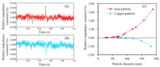
Figure 13.
(a) The relative impedance variation of the 25 μm iron particle, (b) the relative impedance variation of the 66 μm copper particle, and (c) comparison of the induced signals by ferrous and nonferrous particles.
5. Conclusions
We have demonstrated the optimization of a parallel resonance circuit by adjusting the capacitance for wear debris detection in lubricants. Both ferrous and nonferrous particles of fixed sizes were taken under consideration. The relative impedance variations in the resonance circuit due to the passage of particles were first tested for a range of capacitances. Theoretical analysis was conducted as well, which matched well with the experimental results. The relative impedance variation growth curve for the ferrous particles had a sine wave-like shape, and it reached the maximum absolute value at the positive peak. Interestingly, the growth curve of the nonferrous particle had roughly a bell curve-like shape, remaining mostly on the negative side of the axis. The optimal capacitance for the nonferrous particle detection was also found to be larger than that of the ferrous particle. We attribute this difference to the additional resistance increase caused by the eddy current effect. Consequently, we propose using two sensing coils with the optimum capacitors for the ferrous and nonferrous particles on the sensing channel to detect two kinds of particles separately. The study would contribute to the real-time online wear debris detection in lubricant or hydraulic oil. The presented optimization method helps to find the optimal parallel capacitor for the sensing coil with certain excitation frequency and provide an idea for other similar circuit optimization. In the future, the improvement of the throughput and actual oil detection for this method would be developed.
Author Contributions
Conceptualization, X.P. and Z.L.; methodology, S.W. and Z.L.; validation, S.W.; formal analysis, D.Z. and K.Y.; writing—original draft preparation, S.W.; writing, review, and editing, Z.L. and M.K.R.; visualization, F.W.; supervision, Z.L.; project administration, Z.L. and X.P. All authors have read and agreed to the published version of the manuscript.
Funding
This work was supported by the National Natural Science Foundation of China (Grant No. 51909019) and Projects for Dalian Youth Star of Science and Technology (Grant No. 2021RQ037).
Institutional Review Board Statement
Not applicable.
Informed Consent Statement
Not applicable.
Conflicts of Interest
The authors declare no conflict of interest.
References
- Jardine, A.K.S.; Lin, D.; Banjevic, D. A Review on Machinery Diagnostics and Prognostics Implementing Condition-Based Maintenance. Mech. Syst. Signal Process. 2006, 20, 1483–1510. [Google Scholar] [CrossRef]
- Jia, R.; Wang, L.; Zheng, C.; Chen, T. Online Wear Particle Detection Sensors for Wear Monitoring of Mechanical Equipment—A Review. IEEE Sens. J. 2022, 22, 2930–2947. [Google Scholar] [CrossRef]
- Dong, X.T.; Nguyen, M.H.; Lee, D. Algorithm Development for Acoustic Emission Measurement in High-Frequency Ranges and Its Application on a Large Two-Stroke Marine Diesel Engine. Measurement 2020, 162, 107907. [Google Scholar] [CrossRef]
- Nithin, S.K.; Hemanth, K.; Shamanth, V. A Review on Combustion and Vibration Condition Monitoring of IC Engine. Mater. Today Proc. 2021, 45, 65–70. [Google Scholar] [CrossRef]
- Bagavathiappan, S.; Lahiri, B.B.; Saravanan, T.; Philip, J.; Jayakumar, T. Infrared Thermography for Condition Monitoring—A Review. Infrared Phys. Technol. 2013, 60, 35–55. [Google Scholar] [CrossRef]
- Edmonds, J.; Resner, M.S.; Shkarlet, K. Detection of Precursor Wear Debris in Lubrication Systems. In Proceedings of the 2000 IEEE Aerospace Conference. Proceedings (Cat. No.00TH8484), Big Sky, MT, USA, 18–25 March 2000; Volume 6, pp. 73–77. [Google Scholar]
- Wang, Z.; Xue, X.; Yin, H.; Jiang, Z.; Li, Y. Research Progress on Monitoring and Separating Suspension Particles for Lubricating Oil. Complexity 2018, 2018, 9356451. [Google Scholar] [CrossRef]
- Ahn, H.S.; Yoon, E.S.; Sohn, D.G.; Kwon, O.K.; Shin, K.S.; Nam, C.H. Practical Contaminant Analysis of Lubricating Oil in a Steam Turbine-Generator. Tribol. Int. 1996, 29, 161–168. [Google Scholar] [CrossRef]
- Varenberg, M.; Halperin, G.; Etsion, I. Different Aspects of the Role of Wear Debris in Fretting Wear. Wear 2002, 252, 902–910. [Google Scholar] [CrossRef]
- Iwai, Y.; Honda, T.; Miyajima, T.; Yoshinaga, S.; Higashi, M.; Fuwa, Y. Quantitative Estimation of Wear Amounts by Real Time Measurement of Wear Debris in Lubricating Oil. Tribol. Int. 2010, 43, 388–394. [Google Scholar] [CrossRef]
- Zhu, X.; Zhong, C.; Zhe, J. Lubricating Oil Conditioning Sensors for Online Machine Health Monitoring—A Review. Tribol. Int. 2017, 109, 473–484. [Google Scholar] [CrossRef]
- Wu, T.; Wu, H.; Du, Y.; Peng, Z. Progress and Trend of Sensor Technology for On-Line Oil Monitoring. Sci. China Technol. Sci. 2013, 56, 2914–2926. [Google Scholar] [CrossRef]
- Hong, W.; Cai, W.; Wang, S.; Tomovic, M.M. Mechanical Wear Debris Feature, Detection, and Diagnosis: A Review. Chin. J. Aeronaut. 2018, 31, 867–882. [Google Scholar] [CrossRef]
- Du, L.; Zhu, X.; Han, Y.; Zhao, L.; Zhe, J. Improving Sensitivity of an Inductive Pulse Sensor for Detection of Metallic Wear Debris in Lubricants Using Parallel LC Resonance Method. Meas. Sci. Technol. 2013, 24, 075106. [Google Scholar] [CrossRef]
- Du, L.; Zhe, J. Parallel Sensing of Metallic Wear Debris in Lubricants Using Undersampling Data Processing. Tribol. Int. 2012, 53, 28–34. [Google Scholar] [CrossRef]
- Yu, Z.; Zeng, L.; Zhang, H.; Yang, G.; Wang, W.; Zhang, W. Frequency Characteristic of Resonant Micro Fluidic Chip for Oil Detection Based on Resistance Parameter. Micromachines 2018, 9, 344. [Google Scholar] [CrossRef]
- Xie, Y.; Shi, H.; Zhang, H.; Yu, S.; Llerioluwa, L.; Zheng, Y.; Li, G.; Sun, Y.; Chen, H. A Bridge-Type Inductance Sensor With a Two-Stage Filter Circuit for High-Precision Detection of Metal Debris in the Oil. IEEE Sens. J. 2021, 21, 17738–17748. [Google Scholar] [CrossRef]
- Du, L.; Zhe, J. A High Throughput Inductive Pulse Sensor for Online Oil Debris Monitoring. Tribol. Int. 2011, 44, 175–179. [Google Scholar] [CrossRef]
- Du, L. A Multichannel Oil Debris Sensor for Online Health Monitoring of Rotating Machinery. Ph.D. Thesis, Department of Mechanical Engineering, University of Akron, Akron, OH, USA, 2012. [Google Scholar]
- Zhang, H.; Zeng, L.; Teng, H.; Zhang, X. A Novel On-Chip Impedance Sensor for the Detection of Particle Contamination in Hydraulic Oil. Micromachines 2017, 8, 249. [Google Scholar] [CrossRef]
- Li, W.; Bai, C.; Wang, C.; Zhang, H.; Ilerioluwa, L.; Wang, X.; Yu, S.; Li, G. Design and Research of Inductive Oil Pollutant Detection Sensor Based on High Gradient Magnetic Field Structure. Micromachines 2021, 12, 638. [Google Scholar] [CrossRef]
- Zhu, X.; Zhong, C.; Zhe, J. A High Sensitivity Wear Debris Sensor Using Ferrite Cores for Online Oil Condition Monitoring. Meas. Sci. Technol. 2017, 28, 075102. [Google Scholar] [CrossRef]
- Hong, W.; Wang, S.; Tomovic, M.; Han, L.; Shi, J. Radial Inductive Debris Detection Sensor and Performance Analysis. Meas. Sci. Technol. 2013, 24, 125103. [Google Scholar] [CrossRef]
- Hong, W.; Wang, S.; Tomovic, M.M.; Liu, H.; Wang, X. A New Debris Sensor Based on Dual Excitation Sources for Online Debris Monitoring. Meas. Sci. Technol. 2015, 26, 095101. [Google Scholar] [CrossRef]
- Feng, S.; Yang, L.; Qiu, G.; Luo, J.; Li, R.; Mao, J. An Inductive Debris Sensor Based on a High-Gradient Magnetic Field. IEEE Sens. J. 2019, 19, 2879–2886. [Google Scholar] [CrossRef]
- Bai, C.; Zhang, H.; Zeng, L.; Zhao, X.; Ma, L. Inductive Magnetic Nanoparticle Sensor Based on Microfluidic Chip Oil Detection Technology. Micromachines 2020, 11, 183. [Google Scholar] [CrossRef]
- Wang, C.; Bai, C.; Yang, Z.; Zhang, H.; Li, W.; Wang, X.; Zheng, Y.; Ilerioluwa, L.; Sun, Y. Research on High Sensitivity Oil Debris Detection Sensor Using High Magnetic Permeability Material and Coil Mutual Inductance. Sensors 2022, 22, 1833. [Google Scholar] [CrossRef]
- Ren, Y.J.; Zhao, G.F.; Qian, M.; Feng, Z.H. A Highly Sensitive Triple-Coil Inductive Debris Sensor Based on an Effective Unbalance Compensation Circuit. Meas. Sci. Technol. 2019, 30, 015108. [Google Scholar] [CrossRef]
- Hong, W.; Wang, S.; Liu, H.; Tomovic, M.M.; Chao, Z. A Hybrid Method Based on Band Pass Filter and Correlation Algorithm to Improve Debris Sensor Capacity. Mech. Syst. Signal Process. 2017, 82, 1–12. [Google Scholar] [CrossRef]
- Hong, W.; Li, T.; Wang, S.; Zhou, Z. A General Framework for Aliasing Corrections of Inductive Oil Debris Detection Based on Artificial Neural Networks. IEEE Sens. J. 2020, 20, 10724–10732. [Google Scholar] [CrossRef]
- Li, C.; Peng, J.; Liang, M. Enhancement of the Wear Particle Monitoring Capability of Oil Debris Sensors Using a Maximal Overlap Discrete Wavelet Transform with Optimal Decomposition Depth. Sensors 2014, 14, 6207–6228. [Google Scholar] [CrossRef]
- Li, C.; Liang, M. Enhancement of Oil Debris Sensor Capability by Reliable Debris Signature Extraction via Wavelet Domain Target and Interference Signal Tracking. Measurement 2013, 46, 1442–1453. [Google Scholar] [CrossRef]
- Zhu, X.; Du, L.; Zhe, J. An Integrated Lubricant Oil Conditioning Sensor Using Signal Multiplexing. J. Micromechanics Microengineering 2015, 25, 015006. [Google Scholar] [CrossRef]
- Du, L.; Zhu, X.; Han, Y.; Zhe, J. High Throughput Wear Debris Detection in Lubricants Using a Resonance Frequency Division Multiplexed Sensor. Tribol. Lett. 2013, 51, 453–460. [Google Scholar] [CrossRef]
- Du, L.; Zhe, J.; Carletta, J.; Veillette, R.; Choy, F. Real-Time Monitoring of Wear Debris in Lubrication Oil Using a Microfluidic Inductive Coulter Counting Device. Microfluid. Nanofluidics 2010, 9, 1241–1245. [Google Scholar] [CrossRef]
- Wu, S.; Liu, Z.; Yu, K.; Fan, Z.; Yuan, Z.; Sui, Z.; Yin, Y.; Pan, X. A Novel Multichannel Inductive Wear Debris Sensor Based on Time Division Multiplexing. IEEE Sens. J. 2021, 21, 11131–11139. [Google Scholar] [CrossRef]
- Wu, S.; Liu, Z.; Yuan, H.; Yu, K.; Gao, Y.; Liu, L.; Pan, X. Multichannel Inductive Sensor Based on Phase Division Multiplexing for Wear Debris Detection. Micromachines 2019, 10, 246. [Google Scholar] [CrossRef] [PubMed]
- Ren, Y.J.; Li, W.; Zhao, G.F.; Feng, Z.H. Inductive Debris Sensor Using One Energizing Coil with Multiple Sensing Coils for Sensitivity Improvement and High Throughput. Tribol. Int. 2018, 128, 96–103. [Google Scholar] [CrossRef]
- Qian, M.; Ren, Y.J.; Feng, Z.H. Interference Reducing by Low-Voltage Excitation for a Debris Sensor with Triple-Coil Structure. Meas. Sci. Technol. 2020, 31, 025103. [Google Scholar] [CrossRef]
- Du, L.; Zhe, J.; Carletta, J.E.; Veillette, R.J. Inductive Coulter Counting: Detection and Differentiation of Metal Wear Particles in Lubricant. Smart Mater. Struct. 2010, 19, 057001. [Google Scholar] [CrossRef]
- Wu, Y.; Yang, C. Ferromagnetic Metal Particle Detection Including Calculation of Particle Magnetic Permeability Based on Micro Inductive Sensor. IEEE Sens. J. 2021, 21, 447–454. [Google Scholar] [CrossRef]
- Wang, X.; Chen, P.; Luo, J.; Yang, L.; Feng, S. Characteristics and Superposition Regularity of Aliasing Signal of an Inductive Debris Sensor Based on a High-Gradient Magnetic Field. IEEE Sens. J. 2020, 20, 10071–10078. [Google Scholar] [CrossRef]
- Zhu, X.; Du, L.; Zhe, J. A 3×3 Wear Debris Sensor Array for Real Time Lubricant Oil Conditioning Monitoring Using Synchronized Sampling. Mech. Syst. Signal Process. 2017, 83, 296–304. [Google Scholar] [CrossRef]


Publisher’s Note: MDPI stays neutral with regard to jurisdictional claims in published maps and institutional affiliations. |
© 2022 by the authors. Licensee MDPI, Basel, Switzerland. This article is an open access article distributed under the terms and conditions of the Creative Commons Attribution (CC BY) license (https://creativecommons.org/licenses/by/4.0/).