Article

Research on Ultra-Short-Term Load Forecasting Based on Real-Time Electricity Price and Window-Based XGBoost Model

1
Economic and Technological Research Institute of State Grid Shandong Electric Power Company, Jinan 250022, China
2
School of Economics and Management, North China Electric Power University, Beijing 102206, China
*
Author to whom correspondence should be addressed.
Energies 2022, 15(19), 7367; https://doi.org/10.3390/en15197367
Submission received: 23 August 2022 / Revised: 22 September 2022 / Accepted: 3 October 2022 / Published: 7 October 2022

Abstract

:
With the continuous development of new power systems, the load demand on the user side is becoming more and more diverse and random, which also brings difficulties in the accurate prediction of power load. Although the introduction of deep learning algorithms has improved the prediction accuracy to a certain extent, it also faces problems such as large data requirements and low computing efficiency. An ultra-short-term load forecasting method based on the windowed XGBoost model is proposed, which not only reduces the complexity of the model, but also helps the model to capture the autocorrelation effect of the forecast object. At the same time, the real-time electricity price is introduced into the model to improve its forecast accuracy. By simulating the load data of Singapore’s electricity market, it is proved that the proposed model has fewer errors than other deep learning algorithms, and the introduction of the real-time electricity price helps to improve the prediction accuracy of the model. Furthermore, the broad applicability of the proposed method is verified by a sensitivity analysis on data with different sample sizes.

1. Introduction

Power load forecasting is based on the identification of multi-dimensional factors such as technology, economy, policy, and meteorology, and explores the impact mechanisms and the internal logical relationships of various related factors on the power load [1]. Combining the evolutionary trend with the development law of historical power load data, an accurate and scientific prediction of future power load can be achieved. Power load forecasting can be further divided into medium- and long-term power load forecasts, short-term power load forecasts and ultra-short-term power load forecasts [2]. Of these, the time scale of ultra-short-term power load forecasting is from 15 min to hours. Accurate ultra-short-term power load forecasting is helpful in solving problems such as real-time dispatching of the power system and real-time trading in the electricity market [3].
Statistical theory and machine learning methods are commonly used in power load forecasting. The applied models mainly include the ARIMA [4], the least squares support vector machine (LSSVM) [5] and the random forest (RF) [6]. With the continuous development of new power systems, the power consumption data of users present an exponential growth trend. The interaction between power sources, power grids, loads and energy storage is further enhanced, which greatly increases the diversity and randomness of user-side load requirements. Therefore, some scholars have introduced deep learning algorithms into power load forecasting to improve the forecasting accuracy. Muzaffar and Afshar [7] proposed a multi-time-scale power load forecasting model based on a long short-term memory (LSTM) network model. Compared with models such as ARMA, SARIMA and ARMAX, it has a higher performance and prediction accuracy. Li et al. [8] proposed an improved sequence-to-sequence gated recurrent unit (GRU) network, which improved the problems of recurrent neural network gradient disappearance, gradient descent and long LSTM calculation time.
However, the superiority of deep learning algorithms often needs to be reflected in large-capacity and high-volatility sample data. When dealing with small-sample data or data with relatively weak random volatility, the prediction accuracy does not produce significant improvements compared to the traditional statistical methods. Shah and Shroff [9] sampled financial market data and found that the traditional ARIMA model had higher prediction accuracy in each dataset by comparing deep learning algorithms such as LSTM and Transformer. In addition, deep learning models often have a relatively complex spatial network structure, which means that the computational complexity and processing time of the model is greatly improved, but the effectiveness of the model is limited. Nevertheless, by carefully configuring the parameters and inputs of traditional machine learning models, their prediction accuracy and computational efficiency are often no less than deep learning algorithms. Elsayed et al. [10] proposed an improved gradient boosting regression tree model in 2021. Through the refined configuration of the model input, its prediction accuracy and generalization ability are significantly better than those of eight deep learning prediction algorithms proposed at nine top computer conferences such as NeurIPS from 2016 to 2020.
In addition to the model, the selection of input indicators was also one of the key factors affecting the accuracy of power load forecasting. In the existing research, scholars mainly focused on meteorological factors and day-types. Tang et al. [11] proposed an ultra-short-term power load prediction method based on an attention mechanism and a convolutional neural network. Meteorological indicators, such as temperature, humidity and precipitation, were selected as the input variables, which significantly reduced the prediction error. Zhu et al. [12] proposed a hybrid prediction model based on a pattern sequence-based matching method and an extreme gradient boosting which significantly improved the forecasting accuracy through introducing influencing factors such as meteorological indicators and day-types. However, with the continuous development of an electricity spot market, the number of market transaction entities has gradually increased [13]. The introduction of the market-based electricity price mechanism will have a significant impact on the electricity consumption behavior and habits of users, which will make it more difficult to deduce the characteristics of the diversified transaction behaviors of transaction entities, and will increase the difficulty of electricity load forecasting in the spot market environment [14,15]. Therefore, to improve the accuracy of power load forecasting, it is necessary to further consider the impact of real-time electricity prices on power load.
Based on previous research, this paper proposes an ultra-short-term power load forecasting method based on the real-time electricity price and a window-based XGBoost model. On the one hand, by windowing the traditional XGBoost model, the multi-dimensional input variables are converted into a one-dimensional reconstruction vector, which not only reduces the complexity of the model, but also helps the model to capture the autocorrelation effect of the predicted object. On the other hand, by introducing real-time electricity prices, the forecasting accuracy of the ultra-short-term power load forecasting model is significantly improved. The simulation analysis was carried out using actual data from the national electricity market of Singapore (NEMS). The superiority and feasibility of the model proposed in this paper are verified by comparing it with several deep learning algorithms.
The structure of this study is as follows. Section 2 introduces the methodology applied in this paper. Section 3 illustrates the model construction and data preprocessing. Section 4 introduces the case study, and the conclusions are given in Section 5.

2. Methodology

2.1. Traditional XGBoost Model

XGBoost (eXtreme Gradient Boosting) is a boosting learning algorithm proposed by Chen and Guestrin in 2016 [16]. The main principle of XGBoost is to construct a weak classifier through a classification and regression tree (CART) and integrate multiple weak classifiers into a strong classifier [17]. Through multiple iterations, the new tree generated each time can fit the residual of the previous tree, and then revise the previous weak classifier to improve the prediction accuracy of the model [18]. The basic principle of the XGBoost model is shown in Formula (1):
y ^ i = k = 1 K f k ( x i ) f k F
where y ^ i represents the prediction result; K represents the number of decision trees; f k contains the structure q and leaf weight ω of the k -th independent tree; x i represents the i -th input and F represents the function space of the CART regression tree.
The objective function L of the XGBoost model is mainly composed of a loss function and a regularization term, as shown in Formula (2):
{ L = i = 1 n l ( y i , y ^ i ) + k = 1 K Ω ( f k ) Ω ( f k ) = γ T + 1 2 λ ω 2
where l represents the second-order differentiable loss function, which is used to measure the gap between the actual value y i and the predicted value y ^ i ; γ and λ represent the regular term coefficients, which are used to reduce the complexity of the model and prevent the model from overfitting and T represents the number of leaf nodes in the tree model.
Performing Taylor expansion on Formula (2), as shown in Formula (3):
L i = 1 n [ g i f t ( x i ) + 1 2 h i f t 2 ( x i ) ] + γ T + 1 2 λ ω 2 j = 1 T [ ( i I j g i ) ω j + 1 2 ( i I j h i ) ω j 2 ] + γ T
where g i represents the first derivative of x i ; h i represents the second derivative of x i ; t represents the number of iterations; ω j represents the output of the j -th leaf node and I j represents the data sample of the value for the j -th leaf node.
Solve Formula (3) to obtain the optimal leaf weight ω j * and objective function value, as shown in Formula (4):
{ ω j * = G j H j + λ L = 1 2 j = 1 T G j H j + λ + λ T
where G j = i I j g i and H j = i I j h i .

2.2. Window-Based XGBoost Model

The unique tree structure of the XGBoost model makes it perform well when dealing with structured data, but it often loses a certain flexibility when solving time-series forecasting problems. To solve this problem, a window-based XGBoost model (XGBoost(W-b) is proposed in this paper. The basic principle of an XGBoost(W-b) model is to reconfigure time series data as windowed input, and train each window separately, so as to obtain higher prediction accuracy.
First, define the window size W and use the conversion function ϕ to convert the two-dimensional time series input into a one-dimensional vector, as shown in Formula (5):
W × ( L + M ) ( W + M )
where L represents the target channel, which means the number of objects to be predicted. This paper mainly predicts the short-term power load, so L = 1 . M represents the number of selected influencing factors. When only the historical data of the power load are used for prediction without considering other influencing factors, M = 0 .
Through the conversion function, the target values in the window are connected in series. Then, the influence factor vector of the previous time is added to realize the windowed reconstruction of the model inputs. Taking part of the model sample as an example, Figure 1 introduces the basic principle of the XGBoost(W-b) model:
As shown in Figure 1, the XGBoost(W-b) model proposed in this paper performs a structured reconstruction process on the input variables of the model. The reconstruction can convert the original multi-dimensional matrix into a one-dimensional vector and convert the multi-input prediction problem into a simple regression problem, which can help reduce the complexity of the model and improve the computational efficiency.
In addition, the output of traditional machine learning algorithms is mostly single variable. To obtain prediction results on multiple future time scales, it is often necessary to introduce a wrapper multi-output regressor (MOR). The basic principle of a MOR is to introduce a loss function in the process of each output, and to convert the multi-output regression problem into a single-objective problem by summing the losses of each prediction result. However, this approach is equivalent to a mechanical repetition of a single-output regression problem, where the predictions are independent of each other, resulting in the model not benefiting from the underlying relationship between the target variables. However, power load always shows a high time series correlation, and the traditional MOR algorithm will affect the accuracy of the prediction to a certain extent. Through the windowing process in this paper, the “group prediction” of future power load can be realized, which helps to capture the autocorrelation effect in the target variable and makes up for the defect of multi-output independent prediction.

3. Model Construction and Data Preprocessing for Ultra-Short-Term Load Forecasting

3.1. Construction of Ultra-Short-Term Load Forecasting Model Considering Real-Time Electricity Price

First, the raw data of load, real-time electricity price and meteorological factors are collected and preprocessed.
Second, the window size is set, and the original multi-dimensional data are converted into a one-dimensional reconstruction vector as the input variable of the XGBoost(W-b) model.
Finally, the predicted results are compared with other machine learning models and deep learning models to verify the superiority of the XGBoost(W-b) model proposed in this paper. Figure 2 shows the framework of the ultra-short-term power load forecasting model considering real-time electricity prices.

3.2. Data Description and Normalization

The load data and real-time electricity price data used in this paper are all from the NEMS market. The time span is from 1 January 2021 to 7 November 2021, with a time interval of 30 min and a total of 14,925 time points. The descriptive statistics of the data are listed in Table 1. To ensure the prediction accuracy of the model, meteorological factors such as temperature and humidity are also used as input indicators of the model, and the time scale and sample size are the same as the load and electricity price data. All data are divided into sample set, validation set and prediction set according to the ratio of 60%, 20% and 20%, where the validation set is used to prevent the model from overfitting.
To speed up the solution speed and improve the prediction accuracy, the data need to be normalized. The minmax normalization method is used for data preprocessing. The formula is as follows:
x i * = x i x min x max x min
where x i * represents the normalized data; x min represents the minimum value of the sample data; x max represents the maximum value of the sample data.

3.3. Prediction Accuracy Evaluation Index Selection

To test the prediction accuracy of the model proposed in this paper, mean absolute error (MAE), mean absolute percentage error (MAPE) and root mean square error (RMSE) are selected [19]. Three indicators are used as prediction accuracy evaluation indicators, and the formulae are as follows:
ε M A E = 1 n i = 1 n | y i y ^ i |
ε M A P E = 1 n i = 1 n | y i y ^ i | y i 100 %
ε R M S E = 1 n i = 1 n ( y i y ^ i ) 2

4. Case Study

4.1. Parameter Setting

The computer used in the empirical analysis had an i7-1185G7 processor, 32 GB memory, and the simulation platform was Python 3.10.2. The parameter setting of the window-based XGBoost model is listed in Table 2 as follows:
To reflect the superiority of the ultra-short-term forecasting model proposed in this paper, two scenarios, “without considering the real-time electricity price” and “considering the real-time electricity price”, are set up, respectively. In the first scenario, the traditional load influencing factors such as temperature and humidity are taken into consideration, while, in the second scenario, we additionally consider the impact of real-time electricity prices, and use real-time electricity price data as one of the input indicators of the model. The essential difference between the two scenarios is whether the influencing factors cover the real-time electricity price, and other parameter settings remain unchanged.
The prediction accuracy of the XGBoost(W-b) model proposed in this paper is verified by comparing it with several other existing models, including: persistence method, machine learning models (LSSVM and BP network), advanced deep learning algorithms (LSTM and GRU) and the original XGBoost model, and the parameters of the compared models are listed in Table 3. From these, the persistence method is often utilized to establish reference (baseline) models which can then be used for comparison. Since the power load often exhibits obvious periodicity and regularity, the model can be used as a baseline for analysis [20,21]. The persistence method of load forecasting can be described as:
y ^ i = y i Δ i
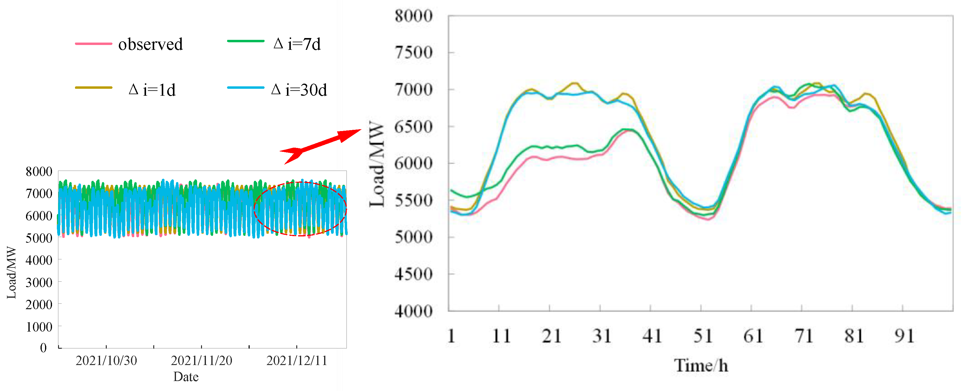
where y i Δ i represents the actual value at time i Δ i . Considering the periodic characteristics of the load data, we set Δ i to be 1 day (24 h), 7 days (168 h) and 30 days (720 h), respectively.
The parameters of the other compared models are set according to the relevant literature. Of which, the e p o c h of LSTM and GRU are set the same as the one of XGBoost, and the b a t c h _ s i z e of LSTM and GRU are set to the same value to ensure consistency (parameters not mentioned are set to default values).
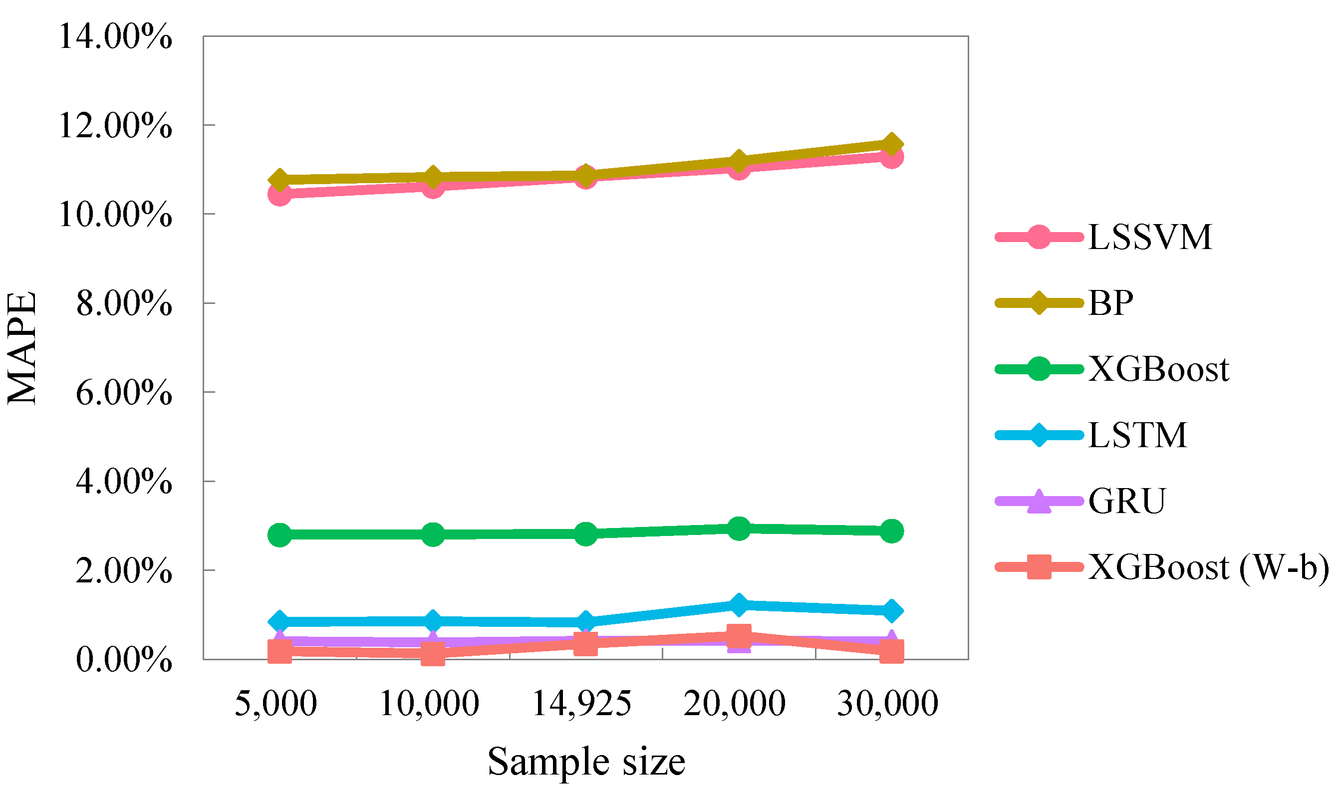
At the same time, to reflect the wider applicability of the model, a sensitivity analysis of the model and the three comparative models are carried out to study the changes in the prediction accuracy of each model when using the sample sizes 5000, 10,000, 20,000 and 30,000.

4.2. Model Prediction Accuracy Based on Persistence Method (Baseline Analysis)

The prediction results and prediction accuracy of persistence method are shown in Figure 3 and Table 4.
As can be seen from Figure 3 and Table 4, load forecasting based on the persistence method can learn the historical evolution law of power load, which has a relatively good performance, especially when Δ i = 7 d .

4.3. Comparison of Model Prediction Accuracy without Considering Real-Time Electricity Prices

Without considering the real-time electricity price, the prediction results and prediction accuracy of each model are shown in Figure 4 and Table 5. Too much data can prevent the clear visualization of the forecast results, so we display the forecast results for the last 100 h separately. The load forecasting part considering the real-time electricity price is the same as the processing method here, and will not be repeated.
It can be seen that, without considering the real-time electricity price, the prediction accuracy ranking of each model is: XGBoost(W-b) > GRU > LSTM > XGBoost > LSSVM > BP. From the MAE point of view, the prediction errors of the XGBoost(W-b) model proposed in this paper are reduced by 90.80%, 91.21%, 86.20%, 67.00% and 65.61%, respectively, compared with the other five models. Meanwhile, we also find that the prediction effect of most models is even lower than the persistence method when the real-time electricity price is not considered. This means that real-time electricity price factors need to be taken into account. In addition, the proposed model is only slightly longer than BP in terms of computation time, which is a significant improvement compared to the other deep learning algorithms.

4.4. Comparison of Model Prediction Accuracy Considering Real-Time Electricity Prices

Considering the real-time electricity price, the prediction results and prediction accuracy of each model are shown in Figure 5 and Table 6:
It can be seen that when considering the real-time electricity price, the prediction accuracy ranking of each model is: XGBoost(W-b) > GRU > LSTM > XGBoost > LSSVM > BP (except that the RMSE of the GRU model is slightly lower than XGBoost(W-b)). From the MAE point of view, the prediction errors of the XGBoost(W-b) model proposed in this paper are reduced by 96.67%, 96.98%, 87.63%, 55.66% and 14.28%, respectively, compared with the other three models. Meanwhile, the computation time of other models is greatly improved due to the increase in the dimension of the input metrics. However, through the windowing method in this paper, even if the real-time electricity price is considered, it does not increase the complexity of the model calculation.

4.5. Sensitivity Analysis

To further verify the applicability of the models proposed in this paper, a sensitivity analysis of each model was carried out. To simplify the analysis, only the changes in MAPE of each model after the sample size change is shown. The results are shown in Figure 6:
As can be seen from Figure 6, the XGBoost(W-b) model proposed in this paper has better performance in most cases. Whether shrinking or expanding the sample size, the prediction error of the model is smaller than that of the traditional XGBoost model and the deep learning algorithm LSTM model. In addition, compared with the GRU model, the model proposed in this paper has a slightly insufficient prediction accuracy when the sample size is expanded to 20,000, but still maintains a high prediction accuracy under other sample sizes. In contrast, traditional machine learning models (LSSVM and BP) seem to perform unsatisfactorily on different sample sizes.

5. Conclusions

With the continuous construction of new power systems and the continuous access of various sources and loads on the user side, the accuracy of load forecasting needs to be further improved. Although deep learning algorithms reduce the prediction error to a certain extent, they have high requirements on sample capacity and data richness and are prone to problems such as high model complexity and low computational efficiency. In this context, this paper proposes a window-based XGBoost model. The effectiveness and superiority of this proposed model were verified through the simulation analysis of NEMS market data. The following conclusions are obtained:
(1)
The introduction of the real-time electricity price has significantly improved the prediction accuracy of the model. The prediction errors of the XGBoost(W-b) model proposed in this paper and the other five comparison models decreased to varying degrees. Even without considering the real-time electricity price, the prediction effect of several models was not even as good as the persistence method. Therefore, the real-time electricity price should be taken into account in the electricity load forecast under the spot market environment;
(2)
Through the windowing transformation of the traditional XGBoost model, the prediction accuracyof this model was significantly improved. In the two scenarios of “without considering the real-time electricity price” and “considering the real-time electricity price”, its performance was no less than that of deep learning algorithms such as LSTM and GRU (commonly used in recent years), and the complexity of the model and the calculation time were also significantly reduced. Therefore, when solving the problem of power load forecasting, the complexity of the model should not be pursued blindly, and a targeted model suitable for the actual problem should be selected. Better performance may be obtained through the careful configuration of the traditional model;
(3)
In addition to the sample set given in this paper, when the sample size is further reduced (1/3 or 2/3 times) or expanded (4/3 or 2 times), the XGBoost(W-b) model proposed in this paper still has a higher prediction accuracy, which reflects the wide applicability of the prediction model proposed in this paper.
The purpose of this paper is to prove that by carefully configuring the input and structure of the model, traditional, simple algorithms can achieve prediction accuracy no less than that of other deep learning algorithms, while simultaneously greatly reducing the required computing time. In the follow-up research, we will introduce the window-based processing method into more traditional models such as the LSSVM and the BP neural network. Meanwhile, we will also try to combine the model algorithm proposed in this paper with other models [25].

Author Contributions

Conceptualization, X.Z. and W.X.; methodology, Y.Z.; software, Y.Z.; validation, H.Z. and S.G.; resources, Q.L.; writing—original draft preparation, Y.Z.; writing—review and editing, H.Z. and S.G.; visualization, Y.Z.; supervision, X.Z. and Q.L.; project administration, W.X. All authors have read and agreed to the published version of the manuscript.

Funding

This research received no external funding.

Data Availability Statement

Not applicable.

Acknowledgments

The authors are grateful to the editor and anonymous reviewers for their work.

Conflicts of Interest

We declare that we do not have any commercial or associative interest that represents a conflict of interest in connection with the work submitted.

References

  1. Zhu, J.; Dong, H.; Zheng, W.; Li, S.; Huang, Y.; Xi, L. Review and prospect of data-driven techniques for load forecasting in integrated energy systems. Appl. Energy 2022, 321, 119269. [Google Scholar] [CrossRef]
  2. He, Y.; Xiao, J.; An, X.; Cao, C.; Xiao, J. Short-term power load probability density forecasting based on GLRQ-Stacking ensemble learning method. Int. J. Electr. Power Energy Syst. 2022, 142, 108243. [Google Scholar] [CrossRef]
  3. Wang, F.; Chen, P.; Zhen, Z.; Yin, R.; Cao, C.; Zhang, Y.; Duić, N. Dynamic spatio-temporal correlation and hierarchical directed graph structure based ultra-short-term wind farm cluster power forecasting method. Appl. Energy 2022, 323, 119579. [Google Scholar] [CrossRef]
  4. Wu, F.; Cattani, C.; Song, W.; Zio, E. Fractional ARIMA with an improved cuckoo search optimization for the efficient Short-term power load forecasting. Alex. Eng. J. 2020, 59, 3111–3118. [Google Scholar] [CrossRef]
  5. Yang, A.; Li, W.; Yang, X. Short-term electricity load forecasting based on feature selection and Least Squares Support Vector Machines. Knowledge-Based Syst. 2018, 163, 159–173. [Google Scholar] [CrossRef]
  6. Fan, G.-F.; Zhang, L.-Z.; Yu, M.; Hong, W.-C.; Dong, S.-Q. Applications of random forest in multivariable response surface for short-term load forecasting. Int. J. Electr. Power Energy Syst. 2022, 139, 108073. [Google Scholar] [CrossRef]
  7. Muzaffar, S.; Afshar, A. Short-Term Load Forecasts Using LSTM Networks. Energy Procedia 2019, 158, 2922–2927. [Google Scholar] [CrossRef]
  8. Li, D.; Sun, G.; Miao, S.; Gu, Y.; Zhang, Y.; He, S. A short-term electric load forecast method based on improved sequence-to-sequence GRU with adaptive temporal dependence. Int. J. Electr. Power Energy Syst. 2021, 137, 107627. [Google Scholar] [CrossRef]
  9. Shah, V.; Shroff, G. Forecasting Market Prices using DL with Data Augmentation and Meta-learning: ARIMA still wins! arXiv 2021, arXiv:2110.10233. [Google Scholar] [CrossRef]
  10. Elsayed, S.; Thyssens, D.; Rashed, A.; Jomaa, H.S.; Schmidt-Thieme, L. Do We Really Need Deep Learning Models for Time Series Forecasting? arXiv 2021, arXiv:2101.02118. [Google Scholar] [CrossRef]
  11. Tang, X.; Chen, H.; Xiang, W.; Yang, J.; Zou, M. Short-Term Load Forecasting Using Channel and Temporal Attention Based Temporal Convolutional Network. Electr. Power Syst. Res. 2022, 205, 107761. [Google Scholar] [CrossRef]
  12. Zhu, K.; Geng, J.; Wang, K. A hybrid prediction model based on pattern sequence-based matching method and extreme gradient boosting for holiday load forecasting. Electr. Power Syst. Res. 2020, 190, 106841. [Google Scholar] [CrossRef]
  13. Zhang, Z.; Lin, S.; Ye, Y.; Xu, Z.; Zhao, Y.; Zhao, H.; Sun, J. A Hybrid MCDM Model for Evaluating the Market-Oriented Business Regulatory Risk of Power Grid Enterprises Based on the Bayesian Best-Worst Method and MARCOS Approach. Energies 2022, 15, 2978. [Google Scholar] [CrossRef]
  14. Guo, X.; Zhao, Q.; Zheng, D.; Ning, Y.; Gao, Y. A short-term load forecasting model of multi-scale CNN-LSTM hybrid neural network considering the real-time electricity price. Energy Rep. 2020, 6, 1046–1053. [Google Scholar] [CrossRef]
  15. Wu, W.; Liao, W.; Miao, J.; Du, G. Using Gated Recurrent Unit Network to Forecast Short-Term Load Considering Impact of Electricity Price. Energy Procedia 2019, 158, 3369–3374. [Google Scholar] [CrossRef]
  16. Yan, Z.; Chen, H.; Dong, X.; Zhou, K.; Xu, Z. Research on prediction of multi-class theft crimes by an optimized decomposition and fusion method based on XGBoost. Expert Syst. Appl. 2022, 207, 117943. [Google Scholar] [CrossRef]
  17. Zhang, S.; Shi, Z.; Wang, G.; Yan, R.; Zhang, Z. Application of the extreme gradient boosting method to quantitatively analyze the mechanism of radon anomalous change in Banglazhang hot spring before the Lijiang Mw 7.0 earthquake. J. Hydrol. 2022, 612, 128249. [Google Scholar] [CrossRef]
  18. Brahim, B.; Majeed, F.; Ewusi, A.; Ahenkorah, I. Residual geochemical gold grade prediction using extreme gradient boosting. Environ. Challenges 2021, 6, 100421. [Google Scholar] [CrossRef]
  19. Ye, Q.; Wang, Y.; Li, X.; Guo, J.; Huang, Y.; Yang, B. A power load prediction method of associated industry chain production resumption based on multi-task LSTM. Energy Rep. 2022, 8, 239–249. [Google Scholar] [CrossRef]
  20. Hou, H.; Liu, C.; Wang, Q.; Wu, X.; Tang, J.; Shi, Y.; Xie, C. Review of load forecasting based on artificial intelligence methodologies, models, and challenges. Electr. Power Syst. Res. 2022, 210, 108067. [Google Scholar] [CrossRef]
  21. Kychkin, A.V.; Chasparis, G.C. Feature and model selection for day-ahead electricity-load forecasting in residential buildings. Energy Build. 2021, 249, 111200. [Google Scholar] [CrossRef]
  22. Zhao, Z.; Zhang, Y.; Yang, Y.; Yuan, S. Load forecasting via Grey Model-Least Squares Support Vector Machine model and spatial-temporal distribution of electric consumption intensity. Energy 2022, 255, 124468. [Google Scholar] [CrossRef]
  23. Wang, Y.; Niu, D.; Ji, L. Short-term power load forecasting based on IVL-BP neural network technology. Syst. Eng. Procedia 2012, 4, 168–174. [Google Scholar] [CrossRef] [Green Version]
  24. Li, Q.; Zhang, X.; Ma, T.; Liu, D.; Wang, H.; Hu, W. A Multi-step ahead photovoltaic power forecasting model based on TimeGAN, Soft DTW-based K-medoids clustering, and a CNN-GRU hybrid neural network. Energy Rep. 2022, 8, 10346–10362. [Google Scholar] [CrossRef]
  25. de Oliveira, J.F.L.; Silva, E.G.; Neto, P.S.G.D.M. A Hybrid System Based on Dynamic Selection for Time Series Forecasting. IEEE Trans. Neural Netw. Learn. Syst. 2021, 33, 3251–3263. [Google Scholar] [CrossRef]
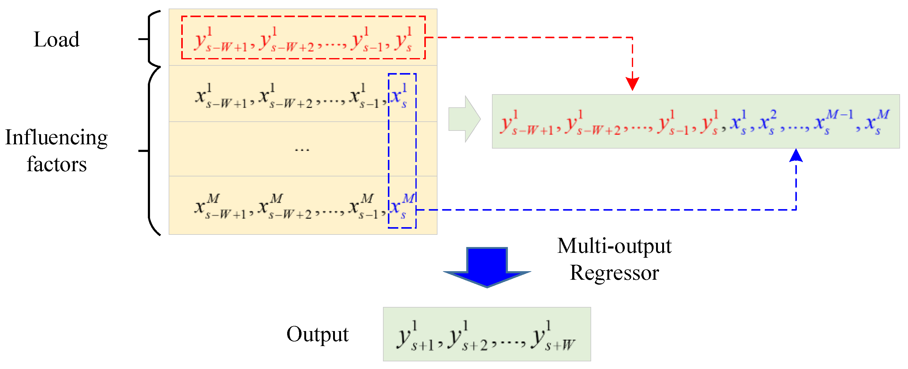
Figure 1. The basic principle of window-based XGBoost model.
Energies 15 07367 g001
Figure 2. Ultra-short-term power load forecasting model considering real-time electricity price.
Energies 15 07367 g002
Figure 3. Load forecasting based on persistence method.
Energies 15 07367 g003
Figure 4. Load forecasting without considering real-time electricity prices.
Energies 15 07367 g004
Figure 5. Load forecasting considering real-time electricity prices.
Energies 15 07367 g005
Figure 6. Sensitivity analysis.
Energies 15 07367 g006
Table 1. The descriptive statistics of the data.
IndicatorObservationAverageMinMaxStd.
Load (MW)14,9256160.194616.937314.83600.21
Electricity Price ($)14,925154.2430.363811.16264.65
Temperature (°C)14,92527.7423.3031.703.50
Humidity (%)14,92584.1882.886.91.30
Table 2. Parameter setting of Window-based XGBoost model.
ParameterValueDescription
W 48Window size
l e a r n i n g _ r a t e 0.025Initial learning rate
g a m m a 0Minimum value of the loss reduction required to specify leaf nodes for branching
m a x _ d e p t h 2Maximum tree depth
n _ e s t i m a t o r s 300Number of decision trees
m i n _ c h i l d _ w e i g h t 1Weight of leaf nodes
s u b s a m p l e 0.9Sub-sample size
c o l s a m p l e _ b y t r e e 0.9Random sampling ratio of features
s c a l e _ p o s _ w e i g h t 0.8Ratio of the number of negative categories to the number of positive categories
s e e d 27Random number seed
Table 3. The parameters setting of the compared models.
ModelParameterValue
LSSVM [22] g a m [0.01, 5000]
s i g 2 [0.01, 100]
BP [23] H i d d e n _ n e u r o n s 10
LSTM e p o c h 300
b a t c h _ s i z e 32
GRU [24] e p o c h 300
b a t c h _ s i z e 32
Table 4. The experimental error of persistence method.
MAEMAPERMSE
Δ i = 1 d 318.393.31%318.39
Δ i = 7 d 219.662.84%219.66
Δ i = 30 d 424.745.08%424.74
Table 5. The experimental error of each model (without considering the real-time electricity price).
MAEMAPERMSEComputation Time
LSSVM697.2411.29%839.5825.70
BP729.9211.82%872.777.63
XGBoost464.927.62%549.1840.36
LSTM194.453.16%255.52271.56
GRU186.602.97%232.47148.10
XGBoost (W-b)64.181.02%96.1112.53
Table 6. The experimental error of each model (considering the real-time electricity price).
MAEMAPERMSEComputation Time
LSSVM660.9810.84%869.5234.10
BP702.1110.87%854.3715.14
XGBoost178.052.82%200.0347.28
LSTM49.670.83%72.93336.00
GRU25.690.41%32.95174.44
XGBoost (W-b)22.020.35%34.2311.48
Publisher’s Note: MDPI stays neutral with regard to jurisdictional claims in published maps and institutional affiliations.