
Qualitative and Quantitative Analysis of the Stability of Conductors in Riserless Mud Recovery System

 ,
,
Abstract
:1. Introduction
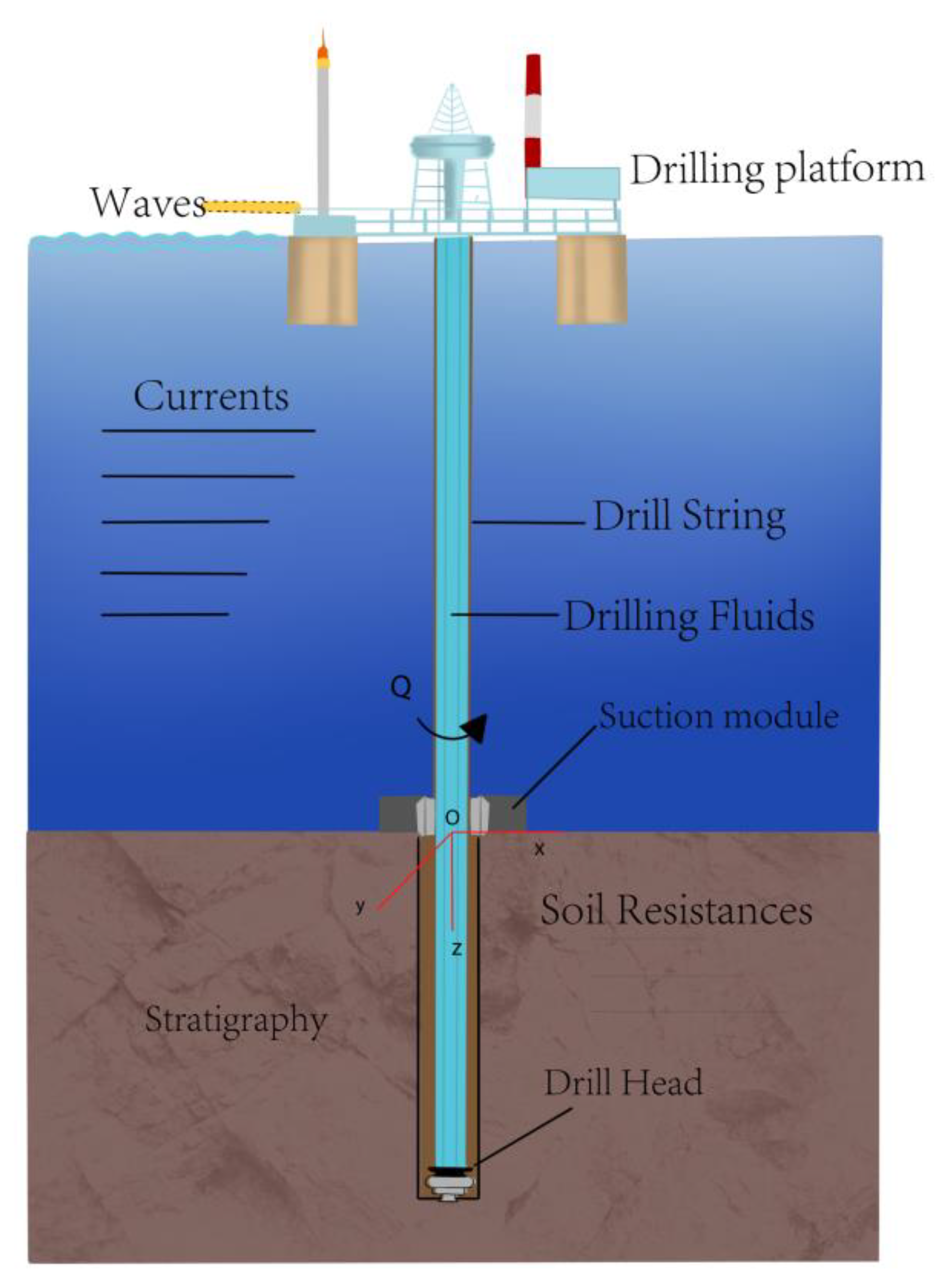
2. RMR Technology
3. Theory and Models
3.1. Conductor Analysis Model
3.2. Simulation Methods for Conductor-Soil Interactions
3.3. Simulation Method of Current Load Effect
3.4. ELM-MIV Weighting Analysis Algorithm
4. Analysis of Factors Influencing the Stability of the Conductor
4.1. Qualitative Analysis of Conductor Stability
4.1.1. Analysis of the Effect of Sea State Recurrence Period on Conductor Stability
4.1.2. Analysis of the Effect of Seabed Soil Properties on Conductor Stability
4.1.3. Analysis of the Influence of Conductor Material on Conductor Stability
4.1.4. Analysis of the Effect of Driving Depth in the Mud on Conductor Stability
4.1.5. Analysis of the Effect of Conductor Wellhead Height on the Stability of the Conductor
4.1.6. Conductor Stability Analysis under Extreme Operating Conditions
4.2. Quantitative Analysis of Factors Influencing the Stability of Conductor
5. Conclusions
- (1)
- Under the selected ultimate conditions, the ultimate displacement of the conductor is 0.5369 m, the ultimate angle of rotation is 2.699 × 10⁻² rad, the ultimate bending moment is 210.2 kN-m, and the ultimate equivalent force is 14.23 MPa, which still meet the operational safety conditions and represent the advantages of RMR technology.
- (2)
- The lateral load of the external environment of the conductor is the major factor affecting the lateral stability of the conductor, so all stability parameters of the conductor will increase with the increase in the sea state recurrence period and the height of the conductor wellhead. Different natures of the seabed soil will lead to different soil resistance of the conductor, the harder the soil, the less the deformation. Conductor materials have too little effect on the conductor stability. As the depth of the conductor in the mud increases, the displacement and angle of rotation of the conductor gradually decrease, while the bending moment and equivalent force first increase and then decrease, with the displacement and angle of rotation increasing sharply when the depth of the conductor in the mud is 10 m.
- (3)
- Sea state recurrence period, conductor wellhead height, and the maximum conductor displacement show a positive correlation. Seabed depth, soil properties, conductor material, and driving depth showed a negative correlation with maximum conductor displacement. The weight values of sea state recurrence period, seabed depth, soil properties, conductor material, driving depth, and conductor wellhead height are 5.01%, 33.14%, 8.62%, 1.52%, 2.97%, and 48.73%, respectively. The factors affecting the conductor stability in descending order are conductor wellhead height, seabed depth, soil properties, sea state recurrence period, driving depth, and conductor material.
Author Contributions
Funding
Data Availability Statement
Conflicts of Interest
Nomenclature
| γc | Unit effective capacity of the soil at depth x under the mud line, kN/m2 |
| Cu | Undrained shear strength of the soil, kPa |
| x | Depth, m |
| D | Diameter of the structure, m |
| ξ | Causeless empirical constant, 0.25–0.5, the soil is hard to take the small value |
| xr | Turning point depth of the ultimate horizontal bearing capacity, m |
| P | Transverse ultimate soil resistance of the structure at the depth x below the mud line when the lateral displacement of the structure occurs, kPa |
| y | Transverse displacement of the structure at the depth x below the mud line, m |
| y50 | Transverse displacement of the structure when the soil transverse soil resistance is half of the ultimate transverse soil resistance, m |
| ε50 | Strain occurring at 1/2 maximum stress in the as-built soil undrained test, m |
| EI | Conductor bending stiffness |
| y | Conductor transverse deformation |
| z | Conductor down into the depth |
| p | Conductor subject to the transverse homogeneous soil resistance |
| fc | Drag force per unit length of the structural member, N |
| ρ | Density of the fluid, kg/m3 |
| CD | Drag force coefficient, 0–150 m below sea level to take 1.2, 150 m below sea level to the sea floor to take 0.7 |
| DC | Hydraulic outside diameter of the structural member, m |
| υ | Velocity of the fluid at the point perpendicular to the structural member, m/s |
| fl | Drag force per unit length of the structural members, N |
| CM | Inertia force coefficient |
| Seawater motion at the calculation point generated by the water quality point acceleration perpendicular to the structural members, m/s2 | |
| β | Weights of the implicit layer neurons and the output neurons |
| H | Implicit layer output matrix |
| T | Output layer matrix |
| w | Weights of input neurons and hidden layer neurons |
| b | Threshold of hidden layer neurons |
| i | Serial number of neurons |
| Y | Training target matrix |
| m | Number of samples |
| t | New output vector value obtained after adding or subtracting a quantity |
Appendix A

| Number | Sea State Recurrence Period (year) | Seabed Depth (m) | Seabed Soil Properties | Conductor Material (Pa) | Driving Depth (m) | Conductor Wellhead Height (m) | Conductor Maximum Displacement (m) |
|---|---|---|---|---|---|---|---|
| 1 | 1 | 10 | 1784066 | 1.9 × 10¹¹ | 40 | 7 | 1.01 × 10⁻² |
| 2 | 10 | 500 | 1784066 | 1.9 × 10¹¹ | 20 | 7 | 5.06 × 10⁻³ |
| 3 | 1 | 1000 | 30156639 | 1.9 × 10¹¹ | 60 | 4 | 7.63 × 10⁻⁵ |
| 4 | 5 | 150 | 1784066 | 1.5 × 10¹¹ | 80 | 9 | 3.79 × 10⁻² |
| 5 | 25 | 10 | 1784066 | 2 × 10¹¹ | 50 | 9 | 1.96 × 10⁻² |
| 6 | 25 | 200 | 30156639 | 1.9 × 10¹¹ | 90 | 9 | 3.87 × 10⁻³ |
| 7 | 5 | 500 | 154022319 | 2.11 × 10¹¹ | 80 | 1 | 3.51 × 10⁻⁵ |
| 8 | 1 | 100 | 30156639 | 1.5 × 10¹¹ | 70 | 6 | 8.48 × 10⁻⁴ |
| 9 | 5 | 250 | 5752930 | 2.11 × 10¹¹ | 20 | 5 | 8.18 × 10⁻³ |
| 10 | 1 | 50 | 1784066 | 2.11 × 10¹¹ | 10 | 2 | 2.01 × 10⁻³ |
| 11 | 5 | 50 | 5752930 | 1.9 × 10¹¹ | 40 | 8 | 7.49 × 10⁻² |
| 12 | 5 | 150 | 154022319 | 1.9 × 10¹¹ | 90 | 8 | 6.59 × 10⁻³ |
| 13 | 1 | 100 | 154022319 | 1.5 × 10¹¹ | 20 | 2 | 1.38 × 10⁻⁴ |
| 14 | 10 | 50 | 30156639 | 2.11 × 10¹¹ | 50 | 7 | 8.94 × 10⁻³ |
| 15 | 10 | 10 | 30156639 | 1.5 × 10¹¹ | 60 | 8 | 1.56 × 10⁻² |
| 16 | 1 | 500 | 154022319 | 2.11 × 10¹¹ | 30 | 9 | 5.90 × 10⁻⁴ |
| 17 | 5 | 300 | 30156639 | 1.9 × 10¹¹ | 20 | 9 | 2.50 × 10⁻³ |
| 18 | 25 | 50 | 5752930 | 1.9 × 10¹¹ | 80 | 4 | 3.63 × 10⁻² |
| 19 | 5 | 1000 | 154022319 | 1.5 × 10¹¹ | 10 | 9 | 1.03 × 10⁻³ |
| 20 | 25 | 250 | 154022319 | 2 × 10¹¹ | 90 | 7 | 2.13 × 10⁻³ |
| 21 | 25 | 1000 | 154022319 | 2.11 × 10¹¹ | 40 | 6 | 4.70 × 10⁻⁴ |
| 22 | 1 | 200 | 5752930 | 2 × 10¹¹ | 20 | 4 | 1.99 × 10⁻³ |
| 23 | 5 | 250 | 1784066 | 1.5 × 10¹¹ | 40 | 3 | 2.24 × 10⁻³ |
| 24 | 1 | 100 | 5752930 | 2 × 10¹¹ | 40 | 9 | 1.13 × 10⁻² |
| 25 | 10 | 300 | 5752930 | 2.11 × 10¹¹ | 50 | 6 | 8.65 × 10⁻³ |
| 26 | 25 | 250 | 30156639 | 2 × 10¹¹ | 60 | 1 | 7.93 × 10⁻⁵ |
| 27 | 25 | 500 | 30156639 | 2 × 10¹¹ | 70 | 2 | 1.19 × 10⁻⁴ |
| 28 | 1 | 500 | 5752930 | 1.9 × 10¹¹ | 90 | 3 | 7.05 × 10⁻⁴ |
| 29 | 1 | 250 | 30156639 | 2 × 10¹¹ | 80 | 8 | 5.47 × 10⁻⁴ |
| 30 | 1 | 250 | 30156639 | 1.9 × 10¹¹ | 50 | 2 | 4.35 × 10⁻⁵ |
| 31 | 10 | 250 | 154022319 | 1.9 × 10¹¹ | 10 | 6 | 1.36 × 10⁻³ |
| 32 | 5 | 1000 | 30156639 | 2.11 × 10¹¹ | 30 | 7 | 4.15 × 10⁻⁴ |
| 33 | 1 | 200 | 1784066 | 1.5 × 10¹¹ | 80 | 7 | 3.44 × 10⁻³ |
| 34 | 25 | 1000 | 1784066 | 1.9 × 10¹¹ | 70 | 3 | 8.72 × 10⁻⁴ |
| 35 | 25 | 100 | 1784066 | 2.11 × 10¹¹ | 50 | 8 | 5.29 × 10⁻² |
| 36 | 1 | 150 | 154022319 | 1.9 × 10¹¹ | 50 | 3 | 1.90 × 10⁻⁴ |
| 37 | 10 | 150 | 5752930 | 2 × 10¹¹ | 70 | 7 | 2.08 × 10⁻² |
| 38 | 10 | 50 | 5752930 | 2 × 10¹¹ | 30 | 3 | 2.09 × 10⁻² |
| 39 | 25 | 200 | 30156639 | 1.5 × 10¹¹ | 30 | 6 | 1.78 × 10⁻³ |
| 40 | 5 | 10 | 154022319 | 2 × 10¹¹ | 70 | 4 | 3.06 × 10⁻³ |
| 41 | 1 | 1000 | 5752930 | 1.5 × 10¹¹ | 90 | 1 | 1.07 × 10⁻⁵ |
| 42 | 1 | 10 | 1784066 | 2.11 × 10¹¹ | 10 | 1 | 2.00 × 10⁻³ |
| 43 | 25 | 250 | 1784066 | 1.5 × 10¹¹ | 30 | 4 | 5.03 × 10⁻³ |
| 44 | 5 | 1000 | 5752930 | 1.5 × 10¹¹ | 50 | 5 | 2.23 × 10⁻³ |
| 45 | 5 | 200 | 30156639 | 2.11 × 10¹¹ | 70 | 8 | 2.17 × 10⁻³ |
| 46 | 1 | 10 | 5752930 | 2 × 10¹¹ | 80 | 6 | 1.20 × 10⁻² |
| 47 | 25 | 50 | 30156639 | 2.11 × 10¹¹ | 20 | 1 | 4.39 × 10⁻⁴ |
| 48 | 5 | 50 | 1784066 | 2 × 10¹¹ | 90 | 6 | 3.02 × 10⁻² |
| 49 | 10 | 300 | 1784066 | 1.9 × 10¹¹ | 70 | 1 | 5.70 × 10⁻⁴ |
| 50 | 1 | 300 | 1784066 | 2 × 10¹¹ | 60 | 5 | 8.96 × 10⁻⁴ |
| 51 | 10 | 1000 | 154022319 | 2 × 10¹¹ | 80 | 2 | 6.00 × 10⁻⁵ |
| 52 | 5 | 200 | 154022319 | 2 × 10¹¹ | 50 | 1 | 7.56 × 10⁻⁵ |
| 53 | 25 | 150 | 5752930 | 2.11 × 10¹¹ | 60 | 2 | 7.69 × 10⁻³ |
| 54 | 10 | 100 | 5752930 | 1.9 × 10¹¹ | 30 | 1 | 4.76 × 10⁻³ |
| 55 | 1 | 150 | 5752930 | 2.11 × 10¹¹ | 20 | 6 | 6.26 × 10⁻³ |
| 56 | 10 | 200 | 1784066 | 1.9 × 10¹¹ | 40 | 2 | 1.60 × 10⁻³ |
| 57 | 25 | 10 | 154022319 | 1.5 × 10¹¹ | 20 | 3 | 2.87 × 10⁻³ |
| 58 | 25 | 150 | 1784066 | 2.11 × 10¹¹ | 30 | 5 | 1.99 × 10⁻² |
| 59 | 10 | 10 | 30156639 | 2.11 × 10¹¹ | 90 | 5 | 4.62 × 10⁻³ |
| 60 | 10 | 1000 | 1784066 | 2 × 10¹¹ | 20 | 8 | 3.41 × 10⁻³ |
| 61 | 10 | 300 | 30156639 | 2.11 × 10¹¹ | 80 | 3 | 2.88 × 10⁻⁴ |
| 62 | 10 | 250 | 5752930 | 2.11 × 10¹¹ | 70 | 9 | 1.87 × 10⁻² |
| 63 | 10 | 500 | 154022319 | 1.5 × 10¹¹ | 50 | 4 | 4.10 × 10⁻⁴ |
| 64 | 10 | 100 | 1784066 | 2.11 × 10¹¹ | 90 | 4 | 1.51 × 10⁻² |
| 65 | 1 | 300 | 154022319 | 2 × 10¹¹ | 30 | 8 | 4.64 × 10⁻⁴ |
| 66 | 25 | 300 | 154022319 | 2.11 × 10¹¹ | 40 | 4 | 5.95 × 10⁻⁴ |
| 67 | 5 | 500 | 1784066 | 1.9 × 10¹¹ | 60 | 6 | 3.11 × 10⁻³ |
| 68 | 10 | 50 | 154022319 | 1.5 × 10¹¹ | 60 | 9 | 2.26 × 10⁻² |
| 69 | 25 | 100 | 5752930 | 1.9 × 10¹¹ | 80 | 5 | 4.09 × 10⁻² |
| 70 | 5 | 150 | 30156639 | 2 × 10¹¹ | 10 | 4 | 1.39 × 10⁻³ |
| 71 | 25 | 200 | 5752930 | 2.11 × 10¹¹ | 60 | 3 | 4.70 × 10⁻³ |
| 72 | 5 | 100 | 154022319 | 1.5 × 10¹¹ | 60 | 7 | 8.64 × 10⁻³ |
| 73 | 25 | 500 | 5752930 | 1.5 × 10¹¹ | 10 | 8 | 4.48 × 10⁻² |
| 74 | 5 | 10 | 5752930 | 1.9 × 10¹¹ | 30 | 2 | 1.19 × 10⁻² |
| 75 | 10 | 500 | 30156639 | 2 × 10¹¹ | 40 | 5 | 4.66 × 10⁻⁴ |
| 76 | 1 | 50 | 154022319 | 1.5 × 10¹¹ | 70 | 5 | 5.86 × 10⁻⁴ |
| 77 | 10 | 150 | 30156639 | 1.5 × 10¹¹ | 40 | 1 | 2.26 × 10⁻⁴ |
| 78 | 10 | 200 | 154022319 | 1.9 × 10¹¹ | 10 | 5 | 1.06 × 10⁻³ |
| 79 | 5 | 100 | 30156639 | 2 × 10¹¹ | 10 | 3 | 1.27 × 10⁻³ |
| 80 | 5 | 300 | 1784066 | 1.5 × 10¹¹ | 90 | 2 | 1.26 × 10⁻³ |
| 81 | 25 | 300 | 5752930 | 1.5 × 10¹¹ | 10 | 7 | 1.93 × 10⁻³ |
References
- Gao, D.; Sun, T.; Zhang, H.; Tang, H. Displacement and Hydraulic Calculation of the SMD System in Ultra-Deep-water Condition. Pet. Sci. Technol. 2013, 31, 1196–1205. [Google Scholar] [CrossRef]
- Lindstrom, J. Ultra-Deep Drilling Cost Reduction; Design and Fabrication of an Ultra-Deep Drilling Simulator (UDS); TerraTek Inc.: Salt Lake City, UT, USA, 2010. [Google Scholar]
- Das, B.; Samuel, R. Reliability Informed Drilling: Analysis for a Dual-Gradient Drilling System. In Proceedings of the SPE Annual Technical Conference and Exhibition, Amsterdam, The Netherlands, 27–29 October 2014; SPE: Amsterdam, The Netherlands, 2014; p. SPE-170815-MS. [Google Scholar]
- Carter, G.; Bland, B.; Pinckard, M. Riserless Drilling-Applications of an Innovative Drilling Method and Tools. In Proceedings of the Offshore Technology Conference, Houston, TX, USA, 2–5 May 2005. [Google Scholar]
- Schubert, J.J.; Juvkam-Wold, H.C.; Choe, J. Well-Control Procedures for Dual Gradient Drilling as Compared to Conventional Riser Drilling. SPE Drill. Complet. 2006, 21, 287–295. [Google Scholar] [CrossRef]
- Forrest, N.; Bailey, T.; Hannegan, D. Subsea Equipment for Deep Water Drilling Using Dual Gradient Mud System. In Proceedings of the SPE/IADC Drilling Conference, Amsterdam, The Netherlands, 27 February–1 March 2001; OnePetro: Richardson, TX, USA, 2001. [Google Scholar]
- Smith, K.L.; Gault, A.D.; Witt, D.E.; Weddle, C.E. SubSea MudLift Drilling Joint Industry Project: Delivering Dual Gradient Drilling Technology to Industry. In Proceedings of the Annual Technical Conference and Exhibition, New Orleans, LA, USA, 30 September–3 October 2001; OnePetro: Richardson, TX, USA, 2001. [Google Scholar]
- Eggemeyer, J.C.; Akins, M.E.; Brainard, R.R.; Judge, R.A.; Peterman, C.P.; Scavone, L.J.; Thethi, K.S. SubSea MudLift Drilling: Design and Implementation of a Dual Gradient Drilling System. In Proceedings of the SPE Annual Technical Conference and Exhibition, New Orleans, LA, USA, 30 September–3 October 2001; OnePetro: Richardson, TX, USA, 2001. [Google Scholar]
- Wilson, A. Taking a Fresh View of Riser Margin for Deep-water Wells Potentially Boosts Safety. J. Pet. Technol. 2013, 65, 93–96. [Google Scholar] [CrossRef]
- Slettebø, D. State and Parameter Identification Applied to Dual Gradient Drilling with Oil Based Mud. Master’s Thesis, Norwegian University of Science and Technology (NTNU), Trondheim, Norway, 2015. [Google Scholar]
- Time, A. Dual Gradient Drilling-Simulations during Connection Operations. Master’s Thesis, University of Stavanger, Stavanger, Norway, 2014. [Google Scholar]
- Haj, A.M. Dual Gradient Drilling and Use of the AUSMV Scheme for Investigating the Dynamics of the System. Master’s Thesis, University of Stavanger, Stavanger, Norway, 2012. [Google Scholar]
- Aird, P. Deep-water “Riserless” Drilling. In Deep-Water Drilling; Elsevier: Amsterdam, The Netherlands, 2019; pp. 441–475. ISBN 978-0-08-102282-5. [Google Scholar]
- Roller, P.R. Riserless Drilling Performance in a Shallow Hazard Environment. In Proceedings of the SPE/IADC Drilling Conference, Amsterdam, The Netherlands, 19–21 February 2003; OnePetro: Richardson, TX, USA, 2003. [Google Scholar]
- Johnson, M.; Rowden, M. Riserless Drilling Technique Saves Time and Money by Reducing Logistics and Maximizing Borehole Stability. In Proceedings of the SPE Annual Technical Conference and Exhibition, New Orleans, LA, USA, 30 September–3 October 2001; OnePetro: Richardson, TX, USA, 2001. [Google Scholar]
- Rezk, R. Safe and Clean Marine Drilling with Implementation of “Riserless Mud Recovery Technology—RMR”. In Proceedings of the SPE Arctic and Extreme Environments Technical Conference and Exhibition, Moscow, Russia, 15–17 October 2013; p. SPE-166839-MS. [Google Scholar]
- Stave, R. Implementation of Dual Gradient Drilling. In Proceedings of the Offshore Technology Conference, Houston, TX, USA, 5–8 May 2014; OnePetro: Richardson, TX, USA, 2014. [Google Scholar]
- Stave, R.; Fossli, B.; Endresen, C.; Rezk, R.H.; Tingvoll, G.I.; Thorkildsen, M. Exploration Drilling with Riserless Dual Gradient Technology in Arctic Waters. In Proceedings of the OTC Arctic Technology Conference, Houston, TX, USA, 10–12 February 2014; OnePetro: Richardson, TX, USA, 2014. [Google Scholar]
- Wang, J.; Sun, J.; Xie, W.; Chen, H.; Wang, C.; Yu, Y.; Qin, R. Simulation and Analysis of Multiphase Flow in a Novel Deep-water Closed-Cycle Riserless Drilling Method with a Subsea Pump + gas Combined Lift. Front. Phys. 2022, 10, 946516. [Google Scholar] [CrossRef]
- Alford, S.E.; Asko, A.; Campbell, M.; Aston, M.S.; Kvalvaag, E. Silicate-Based Fluid, Mud Recovery System Combine to Stabilize Surface Formations of Azeri Wells. In Proceedings of the SPE/IADC Drilling Conference, Amsterdam, The Netherlands, 23–25 February 2005; OnePetro: Richardson, TX, USA, 2005. [Google Scholar]
- Alford, S.E.; Asko, A.; Stave, R.; Aston, M.S.; Kvalvaag, E. Riserless Mud Recovery System and High Performance Inhibitive Fluid Successfully Stabilize West Azeri Surface Formation. In Proceedings of the Offshore Mediterranean Conference and Exhibition, Ravenna, Italy, 16–18 March 2005; OnePetro: Richardson, TX, USA, 2005. [Google Scholar]
- Thorogood, J.L.; Rolland, N.L.; Brown, J.D.; Urvant, V.V. Deployment of a Riserless Mud Recovery System Offshore Sakhalin Island. In Proceedings of the SPE/IADC Drilling Conference, Amsterdam, The Netherlands, 20–22 February 2007; OnePetro: Richardson, TX, USA, 2007. [Google Scholar]
- Thorogood, J.L.; Hogg, T.W.; Kalshikov, A. Exploration Drilling in the Russian Far East: Two Years of Experience and Learning Offshore Sakhalin Island. In Proceedings of the SPE Russian Oil and Gas Technical Conference and Exhibition, Moscow, Russia, 3–6 May 2006; OnePetro: Richardson, TX, USA, 2006. [Google Scholar]
- Opseth, T.L.; Ribesen, B.T.; Tran, T.N.; Hinton, A.; Laget, M.; Lende, G.; Saasen, A. Preventing Shallow Water Flow in North Sea Exploration Wells Possibly Exposed to Shallow Gas. In Proceedings of the Middle East Drilling Technology Conference & Exhibition, Manama, Bahrain, 26–28 October 2009; p. SPE-124608-MS. [Google Scholar]
- Romstad, T.H.; Rogers, H.E.; Saetre, T. Equipment Design Change Improves Cementing Operations from MODUs Operating in Rough Sea Environment: Case Histories for Two North Sea Jobs. In Proceedings of the SPE Asia Pacific Oil and Gas Conference and Exhibition, Brisbane, Australia, 18–20 October 2010; OnePetro: Richardson, TX, USA, 2010. [Google Scholar]
- Claudey, E.; Maubach, C.; Ferrari, S. Deepest Deployment of Riserless Dual Gradient Mud Recovery in Drilling Operation in the North Sea. In Proceedings of the SPE Bergen One Day Seminar, Bergen, Norway, 20 April 2016; p. D011S003R004. [Google Scholar]
- Wiencke, M. The Partnership Between Solution Providers and Oil Companies. In Proceedings of the Offshore Technology Conference, Houston, TX, USA, 30 April–3 May 2007; OnePetro: Richardson, TX, USA, 2007. [Google Scholar]
- Smith, D.; Winters, W.; Tarr, B.; Ziegler, R.; Riza, I.; Faisal, M. Deep-water Riserless Mud Return System for Dual Gradient Tophole Drilling. In Proceedings of the SPE/IADC Managed Pressure Drilling and Underbalanced Operations Conference and Exhibition, Kuala Lumpur, Malaysia, 24–25 February 2010; OnePetro: Richardson, TX, USA, 2010. [Google Scholar]
- Hinton, A.J.; Kvalvaag, E.; Jongejan, A.E.; Seim, K.; Becker, G. BP Egypt Uses RMR on a Jack-up to Solve a Top Hole Drilling–Problem. In Proceedings of the SPE/IADC Drilling Conference and Exhibition, Amsterdam, The Netherlands, 17–19 March 2009; OnePetro: Richardson, TX, USA, 2009. [Google Scholar]
- Jarvis, S.; Grebe, C.; Lively, R. Use of Innovative Technology to Manage Impacts in a Sensitive Environment. APPEA J. 2009, 49, 566. [Google Scholar] [CrossRef]
- Power, M.R. Seismic Expression of Loss Zones within Carbonates of the Browse Basin. In Proceedings of the International Petroleum Technology Conference, Kuala Lumpur, Malaysia, 3–5 December 2008; OnePetro: Richardson, TX, USA, 2008. [Google Scholar]
- Hinton, A.J.; Nolan, T.; Tilley, V.; Eikemo, B. Taming the Grebe Sand—Tophole Drilling Success in the Ichthys Field. In Proceedings of the Asia Pacific Oil and Gas Conference & Exhibition, Jakarta, Indonesia, 4–6 August 2009; p. SPE-121439-MS. [Google Scholar]
- Ali, T.H.; Mathur, R.; Sharma, N. Build-to-Suit Technologies for Wellbore Construction in Deep-water and Ultradeep-water Gulf of Mexico. In Proceedings of the SPE Deepwater Drilling and Completions Conference, Galveston, TX, USA, 5–6 October 2010; p. SPE-136840-MS. [Google Scholar]
- Cohen, J.H.; Kleppe, J.; Grønås, T.; Martin, T.B.; Tveit, T.; Gusler, W.; Christian, C.F.; Golden, S. Gulf of Mexico’s First Application of Riserless Mud Recovery for Top-Hole Drilling—A Case Study. In Proceedings of the Offshore Technology Conference, Houston, TX, USA, 3–6 May 2010; OnePetro: Richardson, TX, USA, 2010. [Google Scholar]
- Goenawan, J.; Goncalves, R.; Dooply, M.; Pasteris, M.; Heu, T.-S.; Chan, L.; Bhaskaran, S.; Hinoul, W. Overcoming Shallow Hazards in Deep-water Malikai Batch-Set Top-Hole Sections with Engineered Trimodal Particle-Size Distribution Cement. In Proceedings of the Offshore Technology Conference Asia, Kuala Lumpur, Malaysia, 22–25 March 2016; OnePetro: Richardson, TX, USA, 2016. [Google Scholar]
- Daniel, M. Use of Riserless Mud Recovery for Protection of Cold Water Corals while Drilling in Norwegian Sea. In Proceedings of the SPE International Conference and Exhibition on Health, Safety, Security, Environment, and Social Responsibility, Stavanger, Norway, 11–13 April 2016; p. D021S023R002. [Google Scholar]
- Rye, H.; Furuholt, E. Validation of Numerical Model for Simulation of Drilling Discharges to Sea. In Proceedings of the Abu Dhabi International Petroleum Exhibition and Conference, Abu Dhabi, United Arab Emirates, 1–4 November 2010; p. SPE-137348-MS. [Google Scholar]
- Jødestøl, K.; Furuholt, E. Will Drill Cuttings and Drill Mud Harm Cold Water Corals? In Proceedings of the SPE International Conference on Health, Safety and Environment in Oil and Gas Exploration and Production, Rio de Janeiro, Brazil, 12–14 April 2010; OnePetro: Richardson, TX, USA, 2010.
- Ong, G.; Yamaguchi, S.; Imai, R. Successful Casing Drilling Experience with Premium Connection for Production Casing Application on a Subsea Well. In Proceedings of the SPE Asia Pacific Oil and Gas Conference and Exhibition, Jakarta, Indonesia, 22–24 October 2013; p. SPE-165786-MS. [Google Scholar]
- Peyton, J.; McPhee, A.; Eikemo, B.; Evans, H.; Utama, B. World First: Drilling with Casing and Riserless Mud Recovery. In Proceedings of the International Petroleum Technology Conference (IPTC 2013), Beijing, China, 26 March 2013; European Association of Geoscientists and Engineers: Utrecht, The Netherlands, 2013. [Google Scholar]
- Myers, G. Ultra-Deepwater Riserless Mud Circulation with Dual Gradient Drilling. Sci. Drill. 2008, 6, 48–51. [Google Scholar] [CrossRef]
- Li, X.; Zhang, J.; Tang, X.; Mao, G.; Wang, P. Study on Wellbore Temperature of Riserless Mud Recovery System by CFD Approach and Numerical Calculation. Petroleum 2020, 6, 163–169. [Google Scholar] [CrossRef]
- Frøyen, J.; Rommetveit, R.; Jaising, H.; Research, S.P.; Stave, R.; Rolland, N.L.; As, A.S. Riserless Mud Recovery (RMR) System Evaluation for Top Hole Drilling with Shallow Gas. In Proceedings of the SPE Russian Oil and Gas Technical Conference and Exhibition, Moscow, Russia, 3–6 October 2006; p. 9. [Google Scholar]
- Kotow, K.J.; Pritchard, D.M. Riserless Drilling with Casing: Deepwater Casing Seat Optimization. In Proceedings of the IADC/SPE Drilling Conference and Exhibition, New Orleans, LA, USA, 2–4 February 2010; p. SPE-127817-MS. [Google Scholar]
- Li, X.; Zhang, J.; Zhao, H.; Zhang, M.; Sun, X.; Wang, P. Study on Lifting Efficiency of Cuttings in Return Line of Riserless Mud Recovery System. In Proceedings of the 2020 9th International Conference on Informatics, Environment, Energy and Applications, New York, NY, USA, 13–16 March 2020; ACM: Amsterdam, The Netherlands, 2020; pp. 20–26. [Google Scholar]
- Wang, C.; Liu, J.; Hou, W.; Wang, A.; Zhang, P. Study on the Effect of Platform Motion Control on Downhole Pressure in Riserless Dual Gradient Drilling. In Proceedings of the 30th International Ocean and Polar Engineering Conference, Virtual, 11–16 October 2020; OnePetro: Richardson, TX, USA, 2020. [Google Scholar]
- Liu, Y.; Fan, H.; Tian, D.; Wen, Z.; Jiang, W.; Ye, Y.; Yu, L. Stability Analysis of Drilling Pipe and Subsea Wellhead for Riserless Drilling in Deepwater. In Proceedings of the 28th International Ocean and Polar Engineering Conference, Sapporo, Japan, 10–15 June 2018; OnePetro: Richardson, TX, USA, 2018. [Google Scholar]
- Mao, L.; Cai, M.; Liu, Q.; Wang, G. Dynamical Simulation of High-Pressure Gas Kick in Ultra-Deepwater Riserless Drilling. J. Energy Resour. Technol. 2021, 143, 063001. [Google Scholar] [CrossRef]
- Wang, G.; Li, W.; Long, Y.; Liu, G.; Li, Y.; Kong, X.; Liu, Q.; Xiao, Y.; Baletabieke, B. Technological Process of the Composite Casing Drilling Technology in Deep-Water Riserless Well Construction. Chem. Technol. Fuels Oils 2022, 58, 95–103. [Google Scholar] [CrossRef]
- Obadina, A. Hydrodynamic Analysis of Drill String in Open Water. Master’s Thesis, University of Stavanger, Stavanger, Norway, 2013. [Google Scholar]
- Franke, K.W.; Rollins, K.M. Simplified Hybrid P-y Spring Model for Liquefied Soils. J. Geotech. Geoenviron. Eng. 2013, 139, 564–576. [Google Scholar] [CrossRef]
- Amar Bouzid, D. Numerical Investigation of Large-Diameter Monopiles in Sands: Critical Review and Evaluation of Both API and Newly Proposed p-y Curves. Int. J. Geomech. 2018, 18, 04018141. [Google Scholar] [CrossRef]
- Morison, J.R.; Johnson, J.W.; Schaaf, S.A. The Force Exerted by Surface Waves on Piles. J. Pet. Technol. 1950, 2, 149–154. [Google Scholar] [CrossRef]
- Peng, L.; Liu, S.; Liu, R.; Wang, L. Effective Long Short-Term Memory with Differential Evolution Algorithm for Electricity Price Prediction. Energy 2018, 162, 1301–1314. [Google Scholar] [CrossRef]
- Zeng, Y.-R.; Zeng, Y.; Choi, B.; Wang, L. Multifactor-Influenced Energy Consumption Forecasting Using Enhanced Back-Propagation Neural Network. Energy 2017, 127, 381–396. [Google Scholar] [CrossRef]
- Li, C.; Duan, L.; Kang, J.; Li, A.; Xiao, Y.; Chikhotkin, V. Weight Analysis and Experimental Study on Influencing Factors of High-Voltage Electro-Pulse Boring. J. Pet. Sci. Eng. 2021, 205, 108807. [Google Scholar] [CrossRef]
- Dong, X.L.; Cao, S.J.; Tang, H.X. Offshore Drilling Manual, 1st ed.; Petroleum Industry Press: Beijing, China, 2011; Chapter 6; ISBN 978-7-5021-7421-7. [Google Scholar]


| Recurrence Period | 1 Year | 5 Years | 10 Years | 25 Years | ||
|---|---|---|---|---|---|---|
| Depth | ||||||
| Current (m/s) | 10 m | 0.68 | 1.40 | 1.49 | 1.59 | |
| 20 m | 0.66 | 1.39 | 1.48 | 1.57 | ||
| 30 m | 0.70 | 1.36 | 1.46 | 1.57 | ||
| 50 m | 0.45 | 1.35 | 1.46 | 1.58 | ||
| 75 m | 0.57 | 1.29 | 1.40 | 1.53 | ||
| 100 m | 0.48 | 1.21 | 1.31 | 1.42 | ||
| 150 m | 0.44 | 0.99 | 1.06 | 1.14 | ||
| 200 m | 0.43 | 0.81 | 0.86 | 0.91 | ||
| 250 m | 0.40 | 0.75 | 0.81 | 0.87 | ||
| 300 m | 0.35 | 0.73 | 0.77 | 0.82 | ||
| 500 m | 0.35 | 0.56 | 0.61 | 0.67 | ||
| 1000 m | 0.30 | 0.41 | 0.45 | 0.49 | ||
| Basic Parameters | Value | Basic Parameters | Value |
|---|---|---|---|
| Seabed depth (m) | 1000 | Poisson’s ratio of 45# steel | 0.26 |
| Conductor length (m) | 94 | Poisson’s ratio of copper-nickel alloy tube | 0.34 |
| Outside diameter of conductor (mm) | 914.4 | Density of Q235 | 7930 |
| Conductor wall thickness (mm) | 38.1 | Density of stainless steel tube | 7850 |
| Seawater density (kg/m3 | 1034 | Density of 45# steel | 7850 |
| Modulus of elasticity of Q235 (GPa) | 210 | Density of copper–nickel alloy tube | 8908 |
| Modulus of elasticity of stainless steel tube (GPa) | 190 | Soil K1 average | 1.78 × 10⁶ |
| Modulus of elasticity of 45# steel (GPa) | 200 | Soil K2 average | 3.02 × 10⁷ |
| Modulus of elasticity of copper-nickel alloy tubes (GPa) | 150 | Soil K3 average | 1.54 × 10⁸ |
| Poisson’s ratio of Q235 | 0.3 | Soil K4 average | 5.75 × 10⁶ |
| Poisson’s ratio of stainless steel tube | 0.3 | Drag force coefficient | 0.7 |
| Ultimate Displacement (m) | Ultimate Corner (rad) | Ultimate Bending Moment (kN·m) | Ultimate Equivalent Stress (MPa) |
|---|---|---|---|
| 0.5369 | 2.699 × 10⁻² | 210.2 | 14.23 |
| Sea State Recurrence Period | Seabed Depth | Soil Properties | Conductor Material | Mud Entry Depth | Height of Conductor Wellhead |
|---|---|---|---|---|---|
| 1 year | 10 m | K1 (1784066) | Q235 (2.11 × 10¹¹) | 10 m | 1 m |
| 5 year | 20 m | K2 (30156639) | 45# steel (2 × 10¹¹) | 20 m | 2 m |
| 10 year | 30 m | K3 (154022319) | stainless steel tube (1.9 × 10¹¹) | 30 m | 3 m |
| 25 year | 50 m | K4 (5752930) | copper-nickel alloy tube (1.5 × 10¹¹) | 40 m | 4 m |
| / | 75 m | / | / | 50 m | 5 m |
| / | 100 m | / | / | 60 m | 6 m |
| / | 150 m | / | / | 70 m | 7 m |
| / | 200 m | / | / | 80 m | 8 m |
| / | 250 m | / | / | 90 m | 9 m |
| / | 300 m | / | / | / | / |
| / | 500 m | / | / | / | / |
| / | 1000 m | / | / | / | / |
| SN | Actual Value | Predictive Value | Serial Number | Actual Value | Predictive Value |
|---|---|---|---|---|---|
| 1 | 1.87 × 10⁻² | 1.85 × 10⁻² | 11 | 8.64 × 10⁻³ | 8.60 × 10⁻³ |
| 2 | 4.10 × 10⁻⁴ | 4.60 × 10⁻⁴ | 12 | 4.48 × 10⁻² | 4.28 × 10⁻² |
| 3 | 1.51 × 10⁻² | 1.53 × 10⁻² | 13 | 1.19 × 10⁻² | 1.29 × 10⁻² |
| 4 | 4.64 × 10⁻⁴ | 4.68 × 10⁻⁴ | 14 | 4.66 × 10⁻⁴ | 4.64 × 10⁻⁴ |
| 5 | 5.95 × 10⁻⁴ | 5.91 × 10⁻⁴ | 15 | 5.86 × 10⁻⁴ | 5.84 × 10⁻⁴ |
| 6 | 3.11 × 10⁻³ | 3.17 × 10⁻³ | 16 | 2.26 × 10⁻⁴ | 2.25 × 10⁻⁴ |
| 7 | 2.26 × 10⁻² | 2.22 × 10⁻² | 17 | 1.06 × 10⁻³ | 1.36 × 10⁻³ |
| 8 | 4.09 × 10⁻² | 4.18 × 10⁻² | 18 | 1.27 × 10⁻³ | 1.24 × 10⁻³ |
| 9 | 1.39 × 10⁻³ | 1.35 × 10⁻³ | 19 | 1.26 × 10⁻³ | 1.29 × 10⁻³ |
| 10 | 4.70 × 10⁻³ | 4.68 × 10⁻³ | 20 | 1.93 × 10⁻³ | 1.99 × 10⁻³ |
| Influencing Factors | MIV Value | Weight Value/% |
|---|---|---|
| Sea state recurrence period | 0.037 | 5.01 |
| Seabed depth | −0.244 | 33.14 |
| Soil properties | −0.063 | 8.62 |
| Conductor material | −0.011 | 1.52 |
| Mud entry depth | −0.022 | 2.97 |
| Height of conductor wellhead | 0.359 | 48.73 |
Publisher’s Note: MDPI stays neutral with regard to jurisdictional claims in published maps and institutional affiliations. |
© 2022 by the authors. Licensee MDPI, Basel, Switzerland. This article is an open access article distributed under the terms and conditions of the Creative Commons Attribution (CC BY) license (https://creativecommons.org/licenses/by/4.0/).
Share and Cite
Qin, R.; Xu, B.; Chen, H.; Lu, Q.; Li, C.; Wang, J.; Feng, Q.; Liu, X.; Wang, L. Qualitative and Quantitative Analysis of the Stability of Conductors in Riserless Mud Recovery System. Energies 2022, 15, 7657. https://doi.org/10.3390/en15207657
Qin R, Xu B, Chen H, Lu Q, Li C, Wang J, Feng Q, Liu X, Wang L. Qualitative and Quantitative Analysis of the Stability of Conductors in Riserless Mud Recovery System. Energies. 2022; 15(20):7657. https://doi.org/10.3390/en15207657
Chicago/Turabian StyleQin, Rulei, Benchong Xu, Haowen Chen, Qiuping Lu, Changping Li, Jiarui Wang, Qizeng Feng, Xiaolin Liu, and Linqing Wang. 2022. "Qualitative and Quantitative Analysis of the Stability of Conductors in Riserless Mud Recovery System" Energies 15, no. 20: 7657. https://doi.org/10.3390/en15207657