Abstract
When a grid section is re-energized after an interruption, the load behaviour can be significantly different from normal operation. In this manuscript, the impact of the phenomenon—known as cold load pickup—is investigated by evaluating 31 time series measured after network outages in Austria and Germany. Its impact on power system restoration and the adequacy of the most common type of simplified model for such investigations is assessed by the time domain simulation of a restoration setting involving the parallel operation of conventional and renewable generation. Parameter distributions are provided for the exponential decay and the delayed exponential decay model with the aim of facilitating meaningful consideration of the phenomenon in time domain simulations of power system restoration. The benefits and limitations of these models are assessed by comparison of time domain simulation results using either the normalized raw data, an exponential decay model or a step-wise active power chance to reflect load behaviour. It is shown that using an exponential decay model leads to higher fidelity of simulation results with respect to the resulting steady-state active power sharing among generators than just applying a step-wise power change in the simulation.
1. Introduction
Power system restoration goes along with special challenges regarding the reconnection of loads that underwent unplanned interruptions. The cold load pickup (CLPU) phenomenon, first described in the context of electric heating [1], refers to loads that interact with some kind of storage and kick in synchronously after an outage. The most prominent examples are thermal loads of heating and cooling systems, as well as the charging of chemical batteries and pumping applications. In normal operation, only a fraction of these loads are active at any given time. When a section of the grid is resupplied after it has been unsupplied for some time, this statistical diversity is lost [2,3,4].
This behaviour needs to be considered in order to assess frequency as well as voltage stability during restoration [5,6,7,8,9,10]. In order to improve the fidelity of time domain simulations in this field, we present an investigation of measurements recorded after 31 actual reconnection events with corresponding outage durations of up to 5.9 h, their fit to simplified models and the adequacy of these models for simulation studies. The main method of assessment is the comparison of time domain simulation results using various model assumptions as well as the application of raw data.
Whereas [8] featured an example of the influence of CLPU on long term voltage stability in a reference power system model for that phenomenon [11], the focus of the current work is on active power frequency control in a power system restoration scenario including renewable generation, similar to the case investigated in [12].
The main contributions of this paper are:
- To provide parameter fits of CLPU models for additional disturbance events beyond those 10 published in [8], now totalling 31 events;
- To provide parameter fits based on actual measurements of a real load composition to the delayed exponential decay model of CLPU according to [13], where it was analytically derived for space heating only;
- To determine the degree to which the load profile, caused by CLPU, can be adequately represented using simplified models and to quantify the impact of these simplifications on simulation results with respect to frequency nadir and active power sharing in the use case demonstrated in [12] with a grid structure similar to [14,15].
Although there are approaches to estimate CLPU online during actual power system restoration [16], the focus of this paper is on the range of behaviours to be considered in studies of power system restoration before the actual event, i.e., in the development and training of power system restoration where the level of tolerable CLPU is determined beforehand and used as an input for decision making [17].
The remainder of this paper is organised as follows: In Section 2, simplified load models for CLPU are described, including a literature review with a focus on the models used in this investigation. Section 3 details the measurement time series used along with selection criteria and the methodology for normalization to allow comparison and model fitting. In Section 4, parameters of the CLPU models are determined, their distribution is presented and the results are discussed with regard to the correlation between the outage duration and CLPU model parameters. In Section 5, the simulation setup for the case study is presented, and in Section 6, simulation results are shown, and the impact of the CLPU in general and the choice of simulation model in particular on the simulation results is investigated, as well as parameter sensitivities. Section 7 concludes this paper with a future outlook.
2. Cold Load Pickup Models
The models in this paper do not feature a distinction between active and reactive power. They are described in terms of active power, which directly translates into apparent and reactive power under the assumption that active and reactive power are proportional, i.e., the power factor is constant. This simplifying assumption is necessary since the requirement of separate measurements of active and reactive power would further limit the number of available measurements. Furthermore, inrush currents are neglected since this phenomenon, despite also occurring on reconnection of feeders, happens at a much faster time scale [10,18].
2.1. Exponential Decay Models
Models featuring an exponential decay of an initial power overshoot plausibly reflect the physical behaviour of a number of relevant loads [3,19].
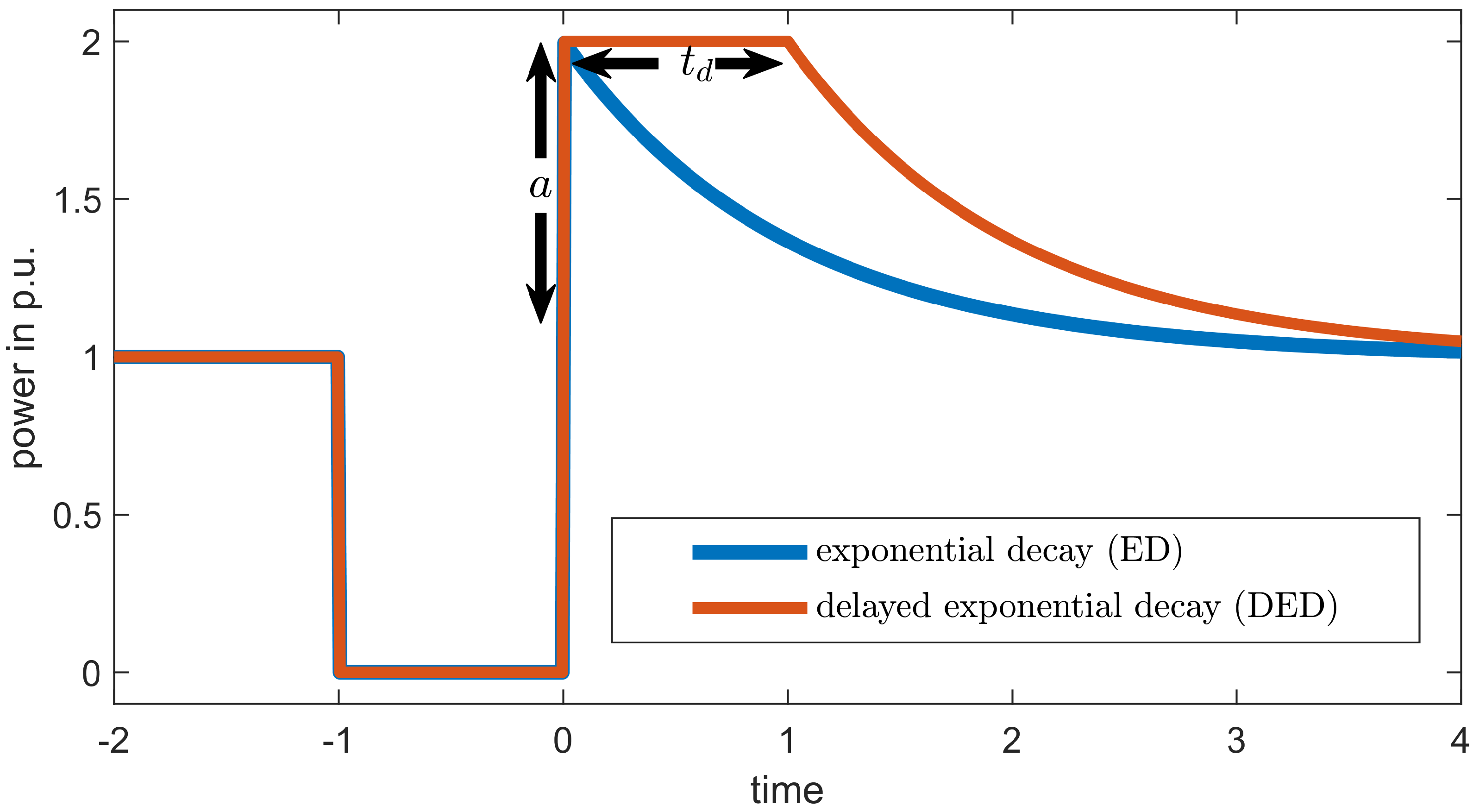
The simplest version of an exponential decay model of CLPU is:
with being the power value expected in normal operation without any disturbance, being the time of reconnection, a being the magnitude of the initial overshoot and its decay time. This model will be called the exponential delay (ED) model for the remainder of this paper.
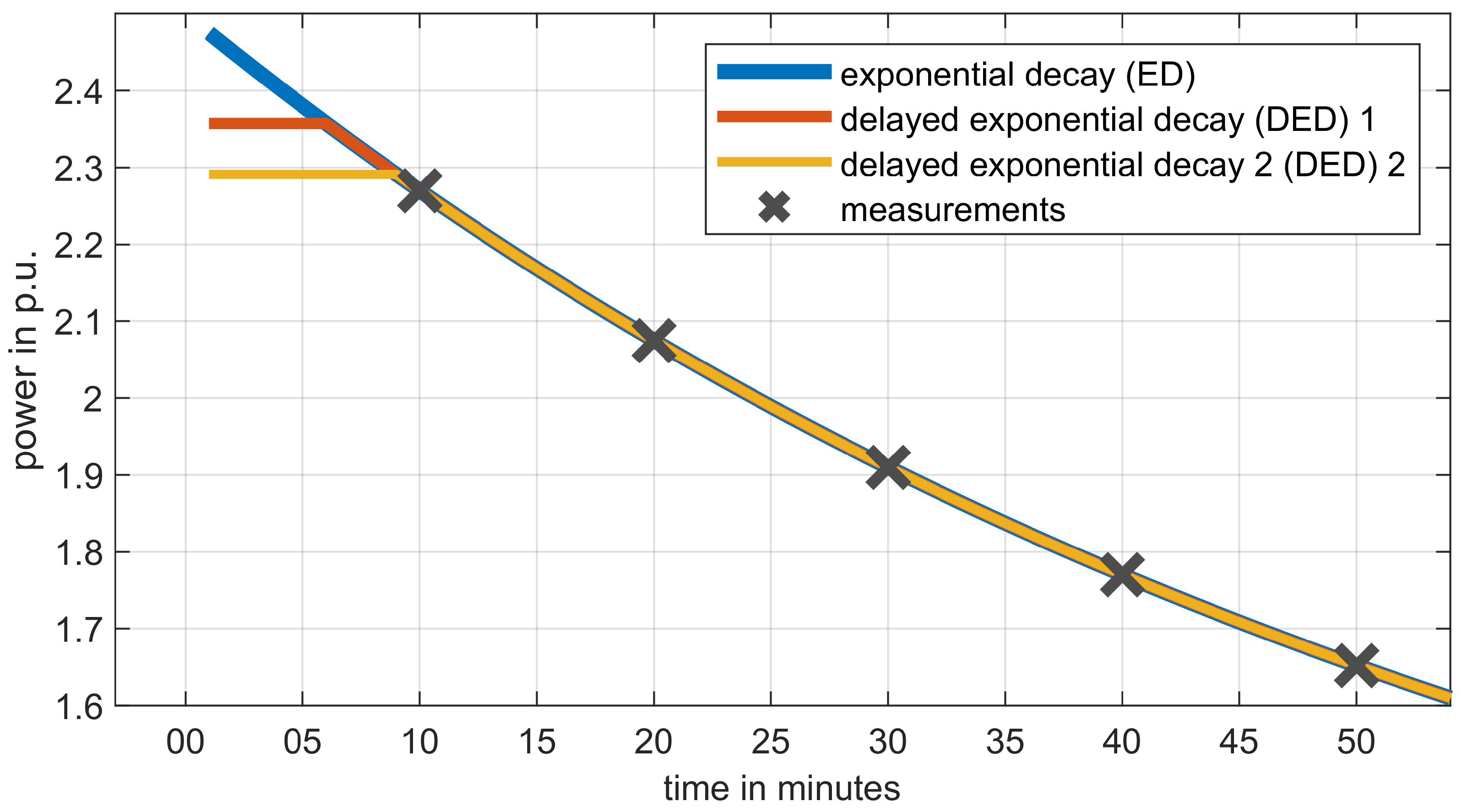
For thermal or battery charging loads, it can be assumed that they will operate at their respective maximum power for a certain time until statistical diversity returns. Therefore, an additional delay parameter has been suggested [4,13] and used for investigations of power system restoration [20,21] as follows:
and
where is the time during which all loads pertinent for CLPU run at full power. Figure 1 shows both curves for the same parameter values of a and . This model will be called the delayed exponential decay (DED) model. If the delay is , it is equivalent to the ED model.
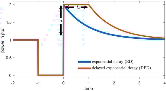
Figure 1.
Exponential decay of CLPU with and without delay, and , or , respectively.
2.2. Other Models
Numerous other models have been suggested to describe the CLPU phenomenon. In [7], a distinction is made between constant loads and manually controlled loads. The latter are assumed to gradually return to their original value via a linear increase after resupply. The same is assumed for industrial processes with a predefined starting sequence [10]. The decrease after the initial overshoot is also sometimes approximated in a linear manner [16]. Detailed physically based models have been introduced for a number of individual loads such as space heating [22,23] and water heating [24]. Furthermore, more complex models have been shown to reflect CLPU more accurately for short outage durations [25]. With detailed knowledge of the individual load composition, power system restoration procedures can even be optimized with regard to the order and timing of reconnections to reduce the impact of CLPU [7,26]. However, the more sophisticated models and optimizations rely on knowledge of the specific loads and, therefore, are hard to apply in a general restoration setting. In order to determine their parameters from electrical measurements only, a vast amount of data would be necessary.
2.3. Interaction of CLPU with Time Variable Demand
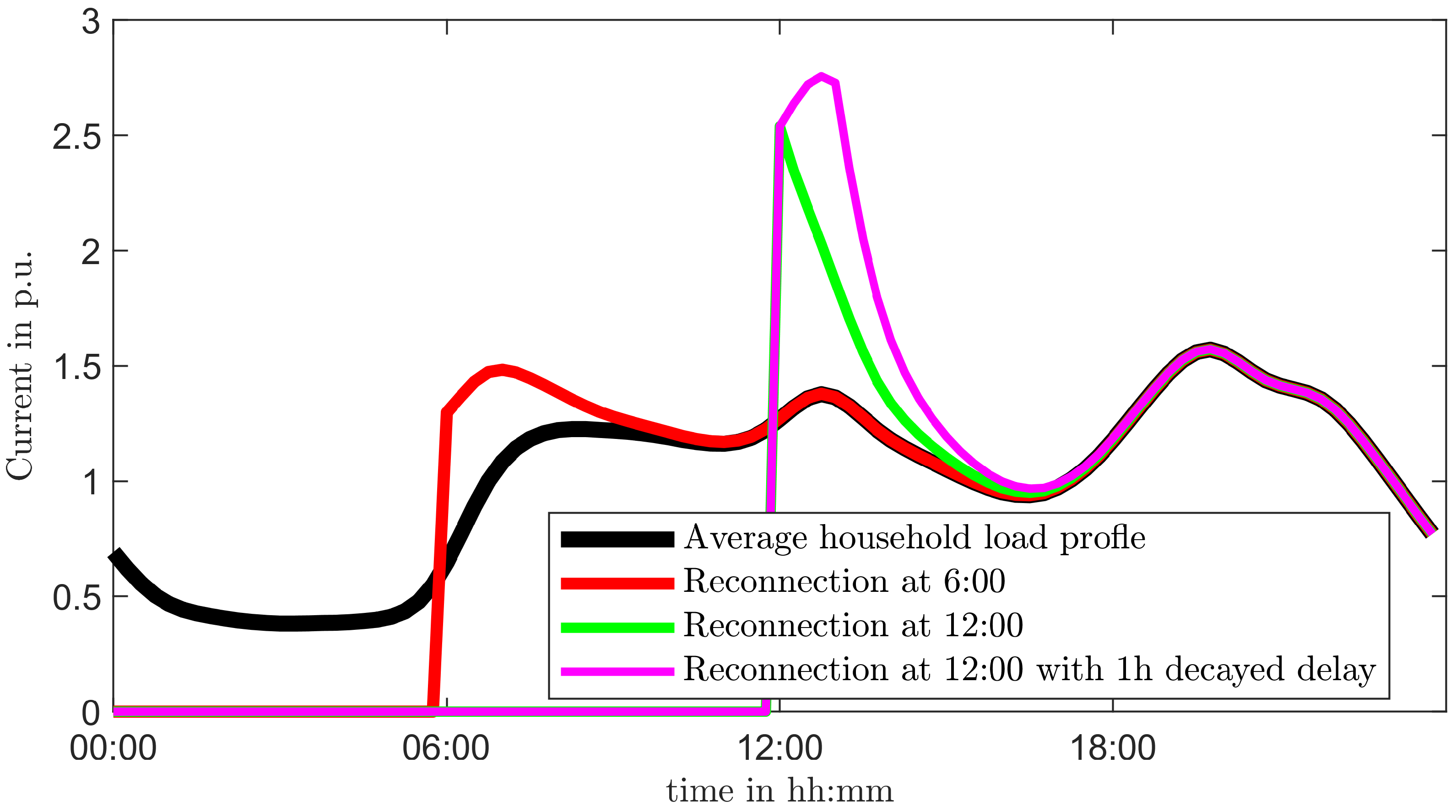
In addition to the interruptions, which are the focus of this paper, load also changes over time during normal operation. Therefore, in order to describe the impact of CLPU on load that would be expected to change even during normal operation, load time series and CLPU models need to be applicable in parallel. The constant then becomes a time-dependent value . Figure 2 shows the example of an average aggregated household load profile [27] subject to the exponential decay models.
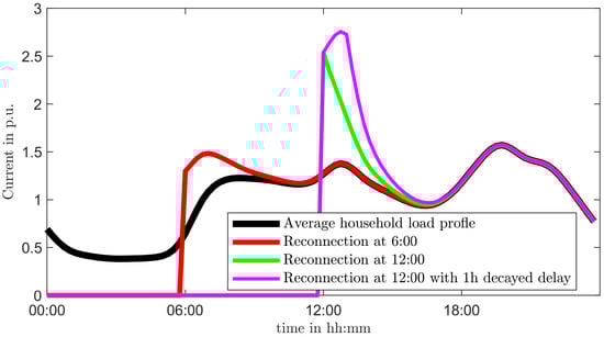
Figure 2.
Combination of time-dependent “normal load” and CLPU with and .
3. Measurement Data
The measurements of current during the reconnection of low and medium-voltage feeders were collected in Austria and Germany between 2012 and 2016. Measurements from Germany were also used for the evaluation in [8]. The additional measurements stem from a study conducted in 2013 in Austria [28].
The minimal requirements for a measurement to be included in this evaluation are the following:
- Outage duration at least 5 min;
- Reconnection after the outage occurred with (nearly) the same switching status as before the disturbance;
- Measurements are available for at least 30 min, requiring an unchanged switching status after reconnection;
- The time resolution of the measurements is at least 1 measurement per minute.
In contrast to [8], the evaluation period after the outage is shorter (30 min instead of two hours) in order to include more measurements. The mean outage duration is 2.1 h, and the maximal outage duration of the events is 5.9 h.
The method of normalization is as in [8]: If sufficient measurements from the same configuration were available for the day before and both days were workdays, a moving one-hour-average around the corresponding time of the day before was assumed to be the normal power. Otherwise, the mean value of all available time spans of undisturbed operation was used. Throughout the remainder of this paper, only normalized time series data are used.
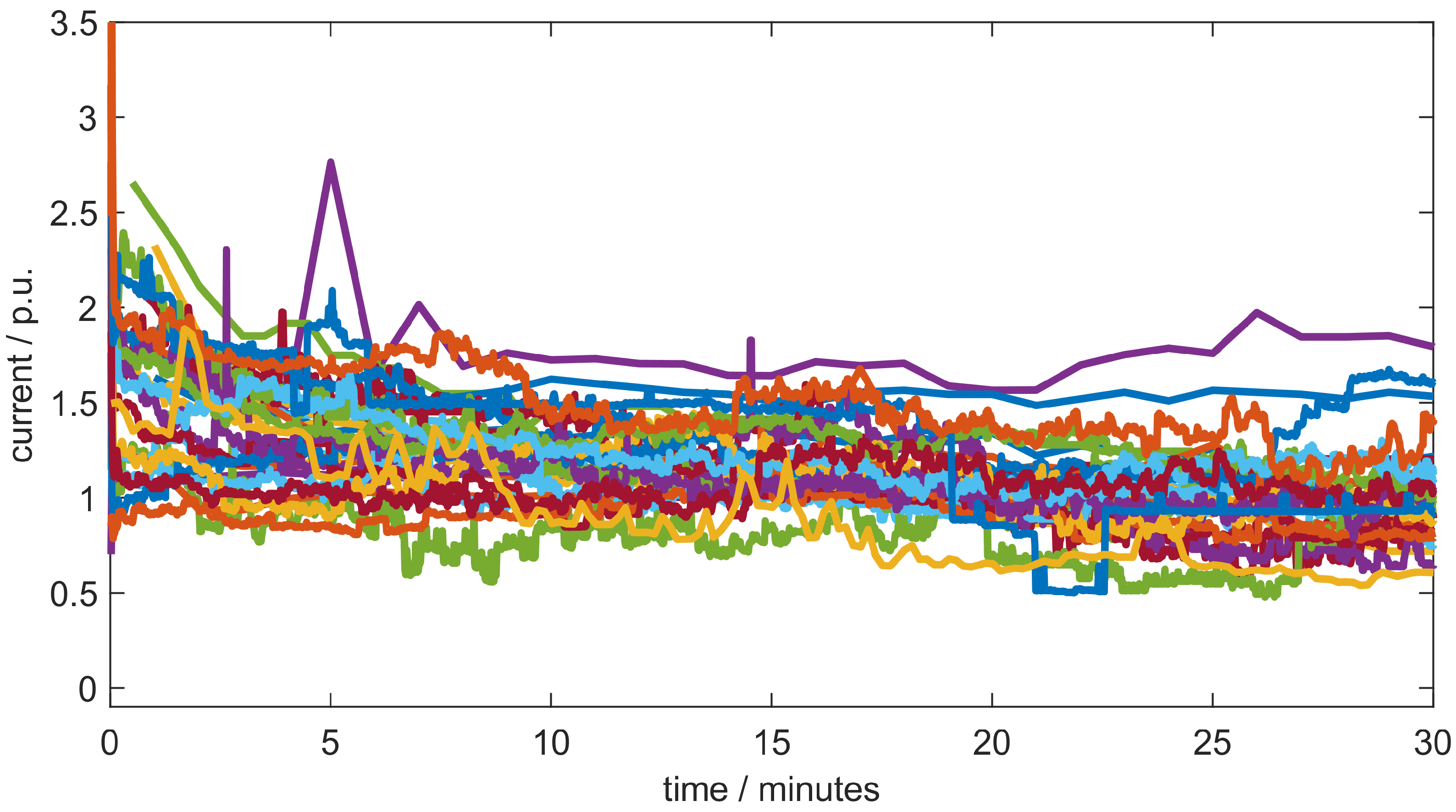
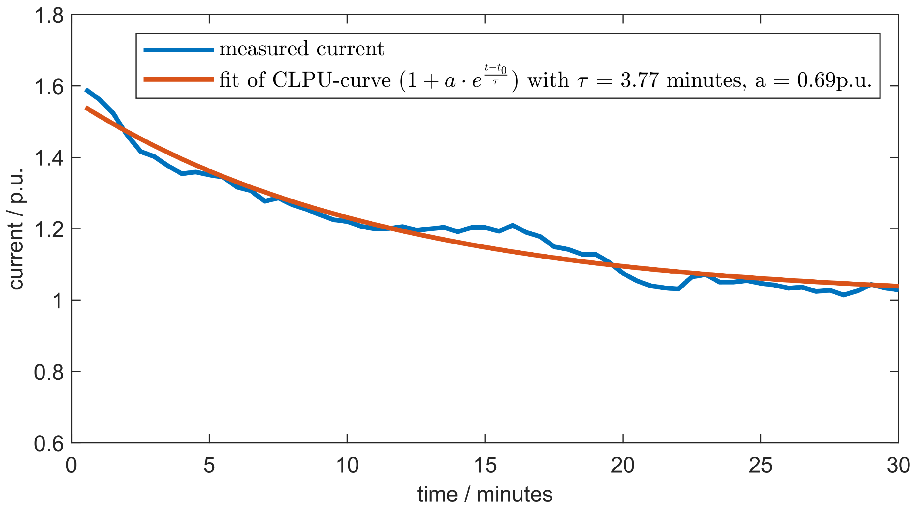
Figure 3 shows the (normalized) current during the recorded events. It can be seen that most cases show increased current immediately after reconnection and then a decay. However, these actual time series are very different from the simplified models. Therefore, the goal of this work is not to determine the goodness of the model fit in a general sense but its adequacy in reflecting certain effects in time domain simulations. Furthermore, the average time series, generated by averaging the respective samples of the 31 events, is qualitatively well reflected by a fit of the exponential decay model, as shown in Figure 4. The root mean square error (RMSE) of the curve fit to the mean of all measurements is 0.030, whereas the mean of the individual RMSEs is 0.119 for the exponential decay model and 0.117 for the delayed exponential decay model.
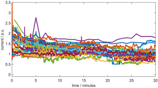
Figure 3.
Normalized current during 31 reconnection events.
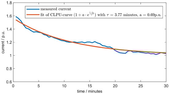
Figure 4.
Normalized mean current of the 31 reconnection events and fitted CLPU curve.
4. Parameter Determination
Model parameters are fitted via the least squares criterion using Matlab. Since only current measurements are available, the parameter fit is performed under the assumption that voltage after reconnection is constant.
4.1. Under-Determined Parameter Fit
For the delayed exponential decay model, there is, by definition, an infinite number of parameter combinations providing an equivalent fit for any limited number of samples: Since
there are multiple combinations of and a yielding the same results, as shown in Figure 5. Therefore, after parameter fitting, is always replaced by the smallest value ≥0 that is equivalent with respect to the measurements.
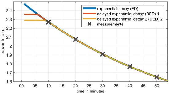
Figure 5.
Example of CLPU curve without delay and with two different values of that fit equally well to measurements.
4.2. Distribution of Parameters
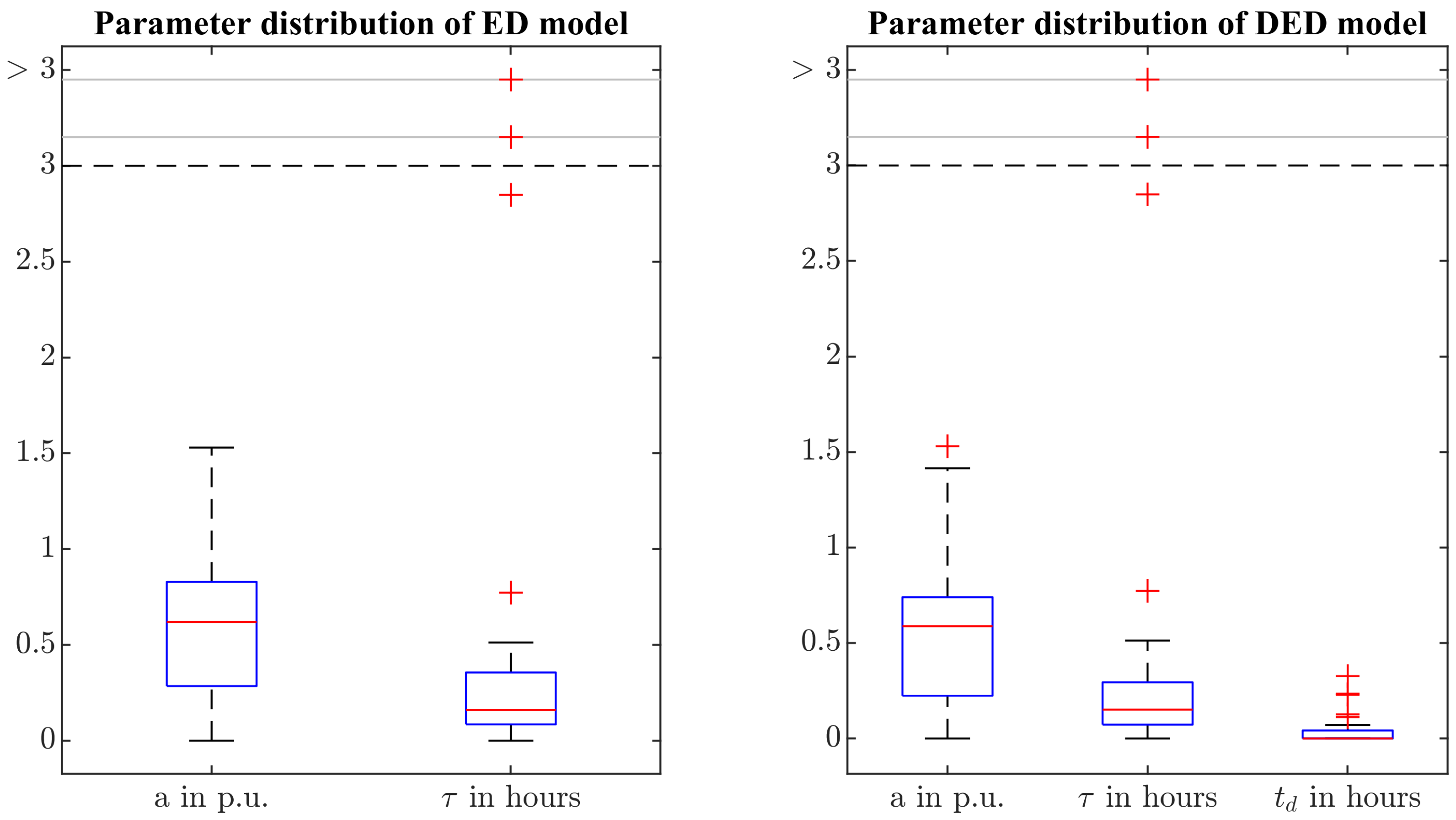
Figure 6 and Table 1 show the distribution of the fitted parameters for the exponential decay models. It can be seen that the overshoot a and the decay time tend to be larger in the ED model than for the DED model. This is to be expected since the delayed exponential decay model allows the same time series in the later stages of CLPU to be reflected with a smaller overshoot a demonstrated in Section 4.1 and also to better fit a slower (or absent) decay early on with a delay instead of a slower decay time.
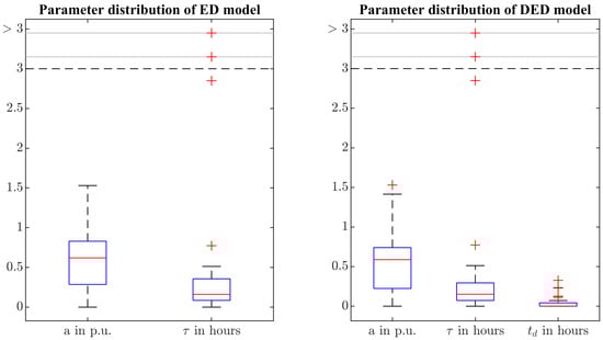
Figure 6.
Distribution of fitted model parameters: Red crosses are outliers beyond 1.5 time the interquartile range. The y-axis is compressed for values beyond 3.

Table 1.
Distribution of fitted model parameters.
However, for most events, the delay is zero or very low, and therefore, both models yield identical or very similar results. This is also reflected in the median of being zero.
The extreme spread of the values results from cases where the measured current does not decrease significantly within the observation period. It should be noted that all but three values are less than one hour for both models. If these three extreme values are excluded, the mean decay time is 12 min for the ED model and 10 min for the DED model.
It should also be noted that the outage durations covered by the available measurements do not include very long outages. Normally, longer outages go along with physical damage, and therefore, reconnection happens step wise, often with provisionally changed topology and does not allow an easy comparison between measurements before and after reconnection. However, in the event of a large-scale blackout and subsequent restoration, reconnection behaviour after longer outages is very relevant. Therefore, power system restoration plans should also consider the possibility of more severe CLPU.
4.3. Correlation of Outage Duration and Parameters
Whereas it is physically plausible that there is some correlation between the outage duration on the one hand and the parameters a, and of the corresponding CLPU event on the other hand [8], no significant correlation could be found within the investigated sample. Table 2 shows the Pearson correlation coefficients for the two models calculated according to Equation (5), where and are the mean values of the parameters or outage durations A and B, respectively, calculated according to Equation (6); and are the corresponding standard deviations calculated by Equation (7); and N is the number of time series. It can be seen that only a very low correlation can be found in the data, none of which passes the significant threshold of . Removing outliers also does not yield significant correlation.
Table 2.
Correlation coefficients of outage duration and parameters of the fitted CLPU model.
Furthermore, external influences such as weather, season, working days or holidays plausibly have a relevant influence on CLPU. However, much more measurement data would be necessary in order to quantify their influence.
5. Simulation Model for Restoration Study
The scenario investigated here is similar to the one presented in [12] and comprises the following:
- Operation of a small island system energized by a blackstart capable gas turbine power plant (blackstart unit, BSU) with a directly coupled synchronous generator and significant renewable generation behaving according to current German grid connection standards for inverter coupled units;
- Active power sharing among generators based on the -characteristics of the generators;
- Reconnection of unsupplied grid areas subject to CLPU.
Parallel operation and active power sharing among gas turbines and renewable energy generation is achieved via the respective active power frequency characteristics of the generation units as described in Section 5.2 and Section 5.3. This mode of operation considers current German grid codes and is possible with most generators currently in the field and also in numerous other countries.
It should be noted that power system restoration is an extraordinary situation in which the usual market mechanisms for coordinating load and generation are not available but the responsible network operator directly gives instructions to (especially larger) generators whereas smaller, automatically reconnecting generators are often not equipped with the necessary functionality for remote control. Furthermore, the ability to aggregate distributed generation in a way that makes handling of all controllable generators feasible is severely limited in a restoration situation. Therefore, the need to manually provide set points to many generators should be minimized.
5.1. System Model
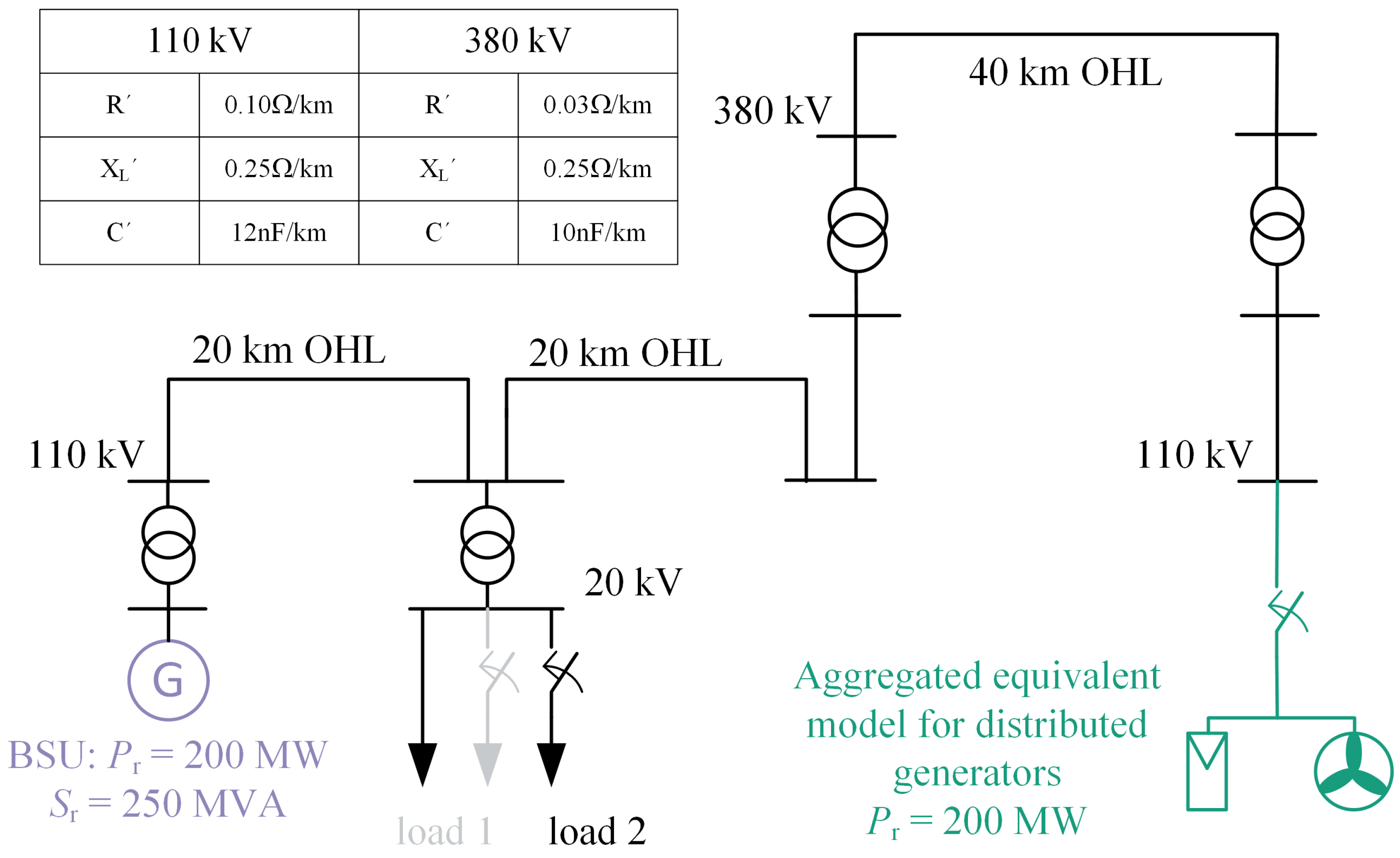
Figure 7 shows the power system used for the simulations, which is typical for the early phase of network restoration. BSU energized parts of the distribution grid consist of overhead lines (OHL) and one circuit of the transmission grid to realize a connection to another high voltage network group including distributed generators with relevant rated power. The distributed generators are connected to their own feeders and can therefore be reconnected independently of load. This is usually the case for generators connected to the high voltage grid and for comparatively large generators connected to the medium voltage grid. Similar results can be expected for the connection of entire medium- and low-voltage grid sections where generation capacity is significantly larger than load. Simulation events are the reconnection of the distributed generators and the reconnection of load 1 and load 2. The models are implemented in Digsilent PowerFactory, and simulations are conducted as effective value simulations (root mean square, RMS) with a step size of 1 ms. Whereas the simulation model of the renewable generation uses a phase-locked loop (PLL) model to determine frequency-dependent control actions, the frequency shown in this paper is the system frequency of the center of inertia, i.e., the angular velocity of the synchronous machine of the gas turbine power plant.
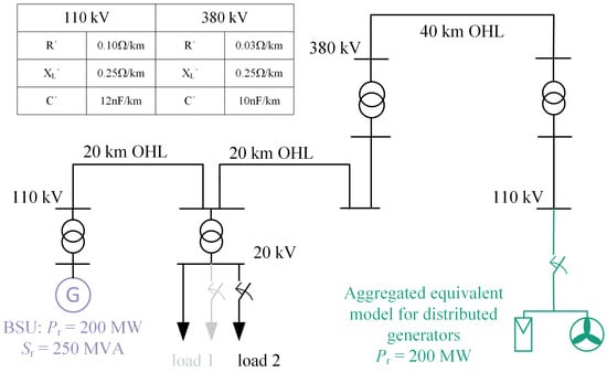
Figure 7.
System model.
5.2. Gas Turbine Power Plant Model
The gas turbine power plant model takes into account a 250 MVA generator with a voltage regulator (AVR) and an IEEE AC1A excitation system [29]. The inertia of the drivetrain (turbine and generator) is considered with a constant start-up time of 10 s. The primary process is realized within the model according to [30]. The controller acting on the gas inlet valve follows a power/frequency curve shown in Figure 8. The droop factor is chosen as 5%, the frequency setpoint is 50 Hz and the active power setpoint is 30.3 MW, corresponding to the initial active power consumption, i.e., load and grid losses. Usually, all thermal power plants, as well as gas turbine power plants, have a technical minimum feed in power that should not be undercut to avoid generator tripping or instability. The explicit value for a specific power plant can be specified by the operator. For the case study, stable operation at active power output of nominal power, i.e., is assumed.
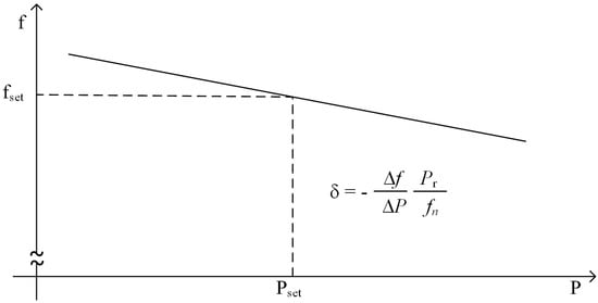
Figure 8.
Droop curve of the power controller.
5.3. Renewable Generation Model
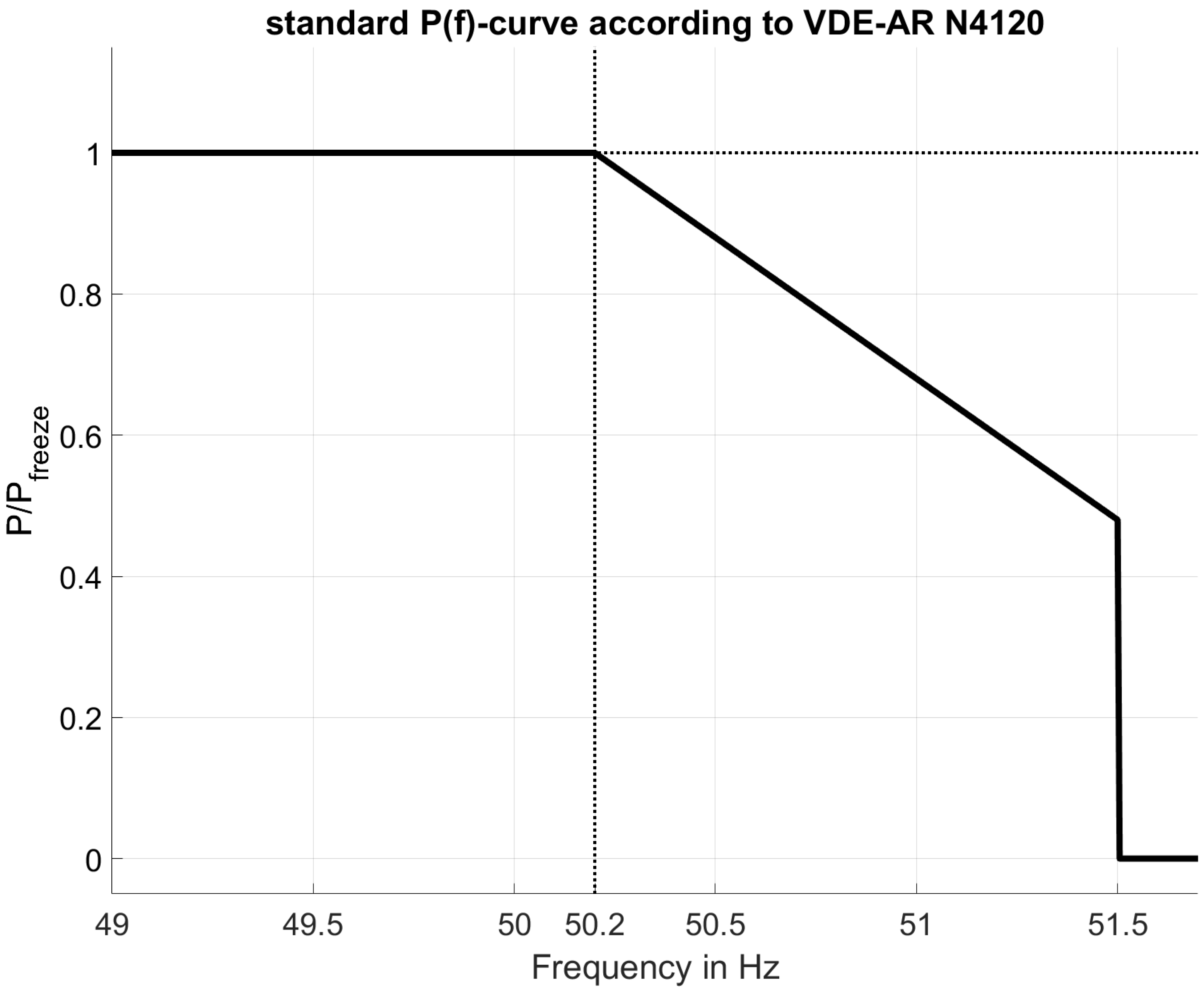
The inverter coupled generation is modeled according to [31,32], implementing the active power frequency, i.e., and reconnection behaviour of the pertinent German grid code [33] for high-voltage connected inverter coupled generation. With respect to the reconnection gradient and -characteristics, this is equivalent to the behaviour of generation connected at lower voltage levels [34,35]. Figure 9 shows the active power reduction at a frequency of over , where is the active power value at the moment when the threshold frequency of was exceeded. The active power ramp rate upon reconnection is limited to 10% of the nominal power per minute. The same limit applies for the continued active power ramp when the frequency falls below 50.2 Hz after an over frequency event. The nominal power of the renewable generation is 200 MW, and the available active power is considered to be high enough to not limit feed in, i.e., larger than 45 MW. The generator will reconnect when the voltage and frequency are within their respective limits for one minute.

Figure 9.
Active power characteristic of renewable generation at over frequency.
It should be noted that the grid codes leave significant room for different implementations by the manufacturers. For example, a slower active power ramp rate after reconnection is also allowed since only an upper limit for the rate is defined in [33,34,35]. The purpose of the implementation presented here is to roughly approximate the aggregated behaviour of one or more wind and/or photovoltaic (PV) plants with the respective total power.
5.4. Load Model
The CLPU of the load is considered as described above for a range of parameters as described in Section 6.2. The resulting power values are multiplied by a voltage and frequency dependency as follows according to [31,36]. These dependencies represent a combination of loads with very different voltage and frequency dependencies such as power electronically coupled loads, resistive loads, directly coupled asynchronous machines, etc.:
and
with , and = 1%/Hz.
6. Simulation Case Study
In the simulation, the renewable generation (200 MW nominal power) is connected at , and the load is connected at and at . The times are chosen to reflect the case that fast dynamics have decayed before the next load connection, whereas the load decay from CLPU is still ongoing.
6.1. Base Case without Any CLPU
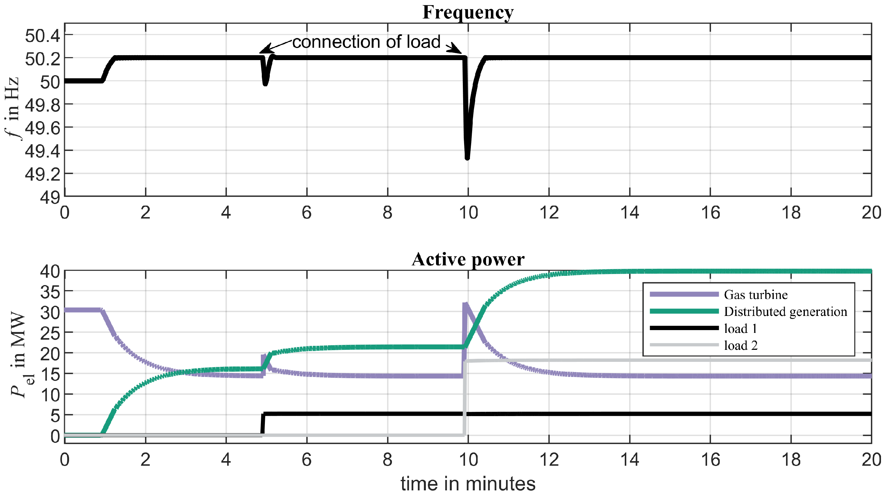
Figure 10 shows the active power ramp up of the distributed generators, followed by the subsequent connection of two loads, the first with 5 MW and the second with 17.5 MW. It can be seen that the renewable generation increases its active power feed-in until the frequency has increased to 50.2 Hz. After each load connection, the active power increases again until a new steady state at is reached and the gas turbine is again feeding-in nearly the same active power as before the load connection (all values between 14.3 MW and 14.4 MW).
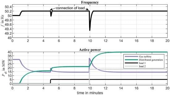
Figure 10.
Base case simulation of load connection with 5 MW and 17.5 MW, respectively.
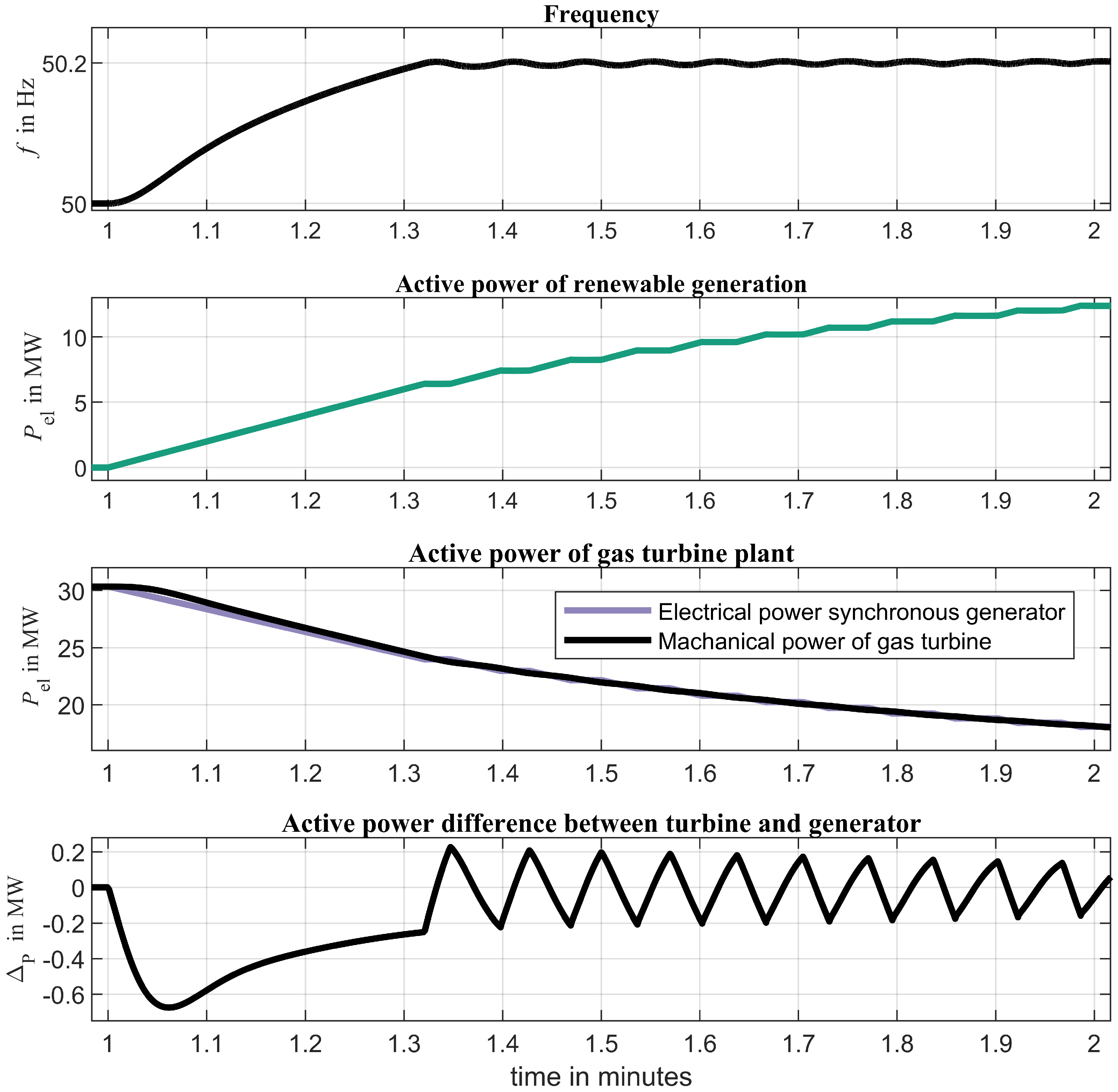
It can be seen that after the frequency has returned to about 50.2 Hz, active power generation still shifts from the synchronous machine to the renewable generator. The reason for this is the slower dynamics of the droop controlled gas turbine that decreases its power further, making the frequency temporarily fall below 50.2 Hz followed by another active power increase in the renewable generation. Figure 11 shows the frequency and power of the renewable generation for the initial ramp up in a higher zoom level. Frequency changes are caused by the active power imbalance between the electrical power of the synchronous machine and the mechanical power applied to the gas turbine. Whenever , it is , and frequency increases. As soon as , the renewable generation stops increasing its active power feed in, thereby stopping the decrease in of the synchronous machine; conversely, the slower turbine decreases its active power until and frequency decreases again. After a few minutes, a stable equilibrium with nearly constant active powers is reached, as can be seen in Figure 10. It should be noted that the controls of the renewable generation unit reacts to local PLL measurements of the frequency at the respective connection point. During transients, these measurements are slightly different from the system frequency shown in the plots.
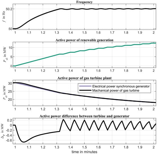
Figure 11.
Frequency and active power of renewable generation.
6.2. Comparison Case with CLPU
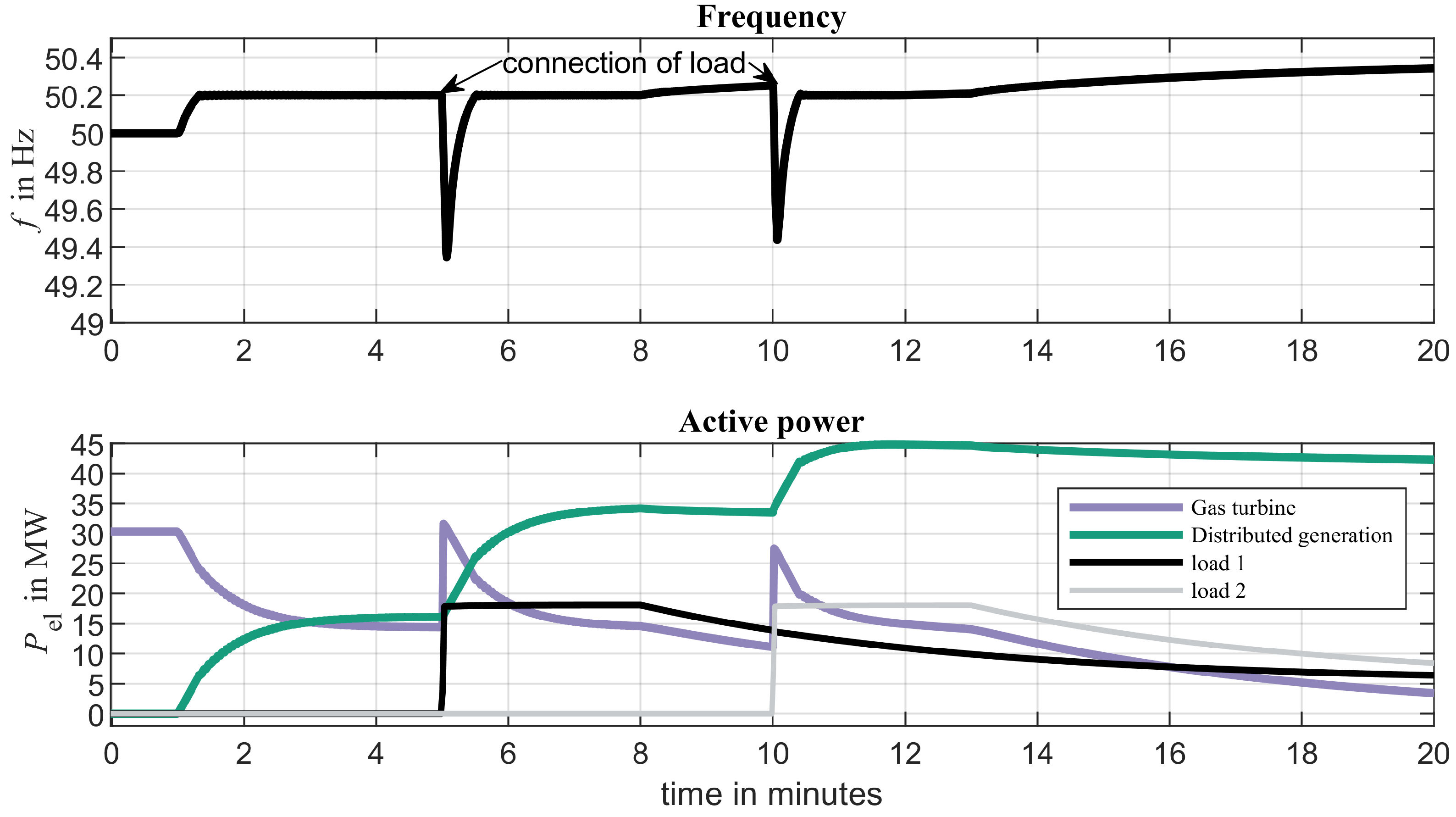
Figure 12 shows the simulation results of the same case but with an added CLPU so that each load has an initial power of 17.5 MW and a steady-state power of 5 MW. It can be seen that the frequency nadir is similar to the results above when a static load of 17.5 MW was connected at 10 min. However, the steady-state operating point of the gas turbine is at significantly lower active power (less than 3.4 MW at 20 min). This can go along with the violation of the minimum active power for the stable operation of the synchronous generator and even its disconnection, leading to a collapse of the island system. It should be noted that the value of used in the example is well beyond the range of CLPU overshoot values encountered in the actual measurements. However, the phenomenon is not limited to such extreme values. Furthermore, a trend towards an increased penetration of electrochemical battery storages as well as thermal loads (esp. heat pumps) might go along with an increased CLPU, and actual power system restoration entails not just two but many more load connection events. Operators should be aware that in such a situation, even the connection of pure load (without any additional distributed generation) might decrease plant loading.
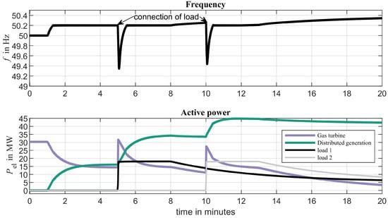
Figure 12.
Base case simulation of load connection subject to CLPU (, , and ).
Whereas the renewable generator does slightly decrease its active power feed-in during over frequency events, it remains well above its steady-state value before the load connection under CLPU conditions. Even with an increase in frequency to 51.5 Hz, the active power feed-in would still be of the active power feed-in before the over frequency event according to the characteristic shown in Figure 9. Since generators are allowed to disconnect at according to [33,34,35], this poses a severe risk for grid collapse.
The challenge of having to deal with decreasing load is hardly exclusive to CLPU, and operators have to be prepared to counter it by changing power set points of generators anyway. However, decreasing generator loading within a few minutes while only connecting load puts additional stress on network operators in a restoration situation and, therefore, should be considered when making power system restoration plans.
6.3. Sensitivity Study: Variation of CLPU Modelling and Parameters
In this section, simulation results are presented for five different approaches to considering CLPU that were applied to each of the 31 events individually:
- Application of recorded current time series;
- Exponential decay (ED) model;
- Delayed exponential decay (DED) model;
- Active power step to the expected initial load;
- Active power step directly to the expected steady-state load value.
For (1), the loads are simulated according to the recorded current time series multiplied by 5 MW. For (2) and (3), the loads are simulated to behave according to the respective CLPU model fitted to each event with according to Equation (1) or Equation (2), respectively. For (4), the loads are simulated as constant loads with , where a is the active power overshot from the ED model, according to Equation (1), fitted to the respective recorded current time series. For (5), correspondingly, load is constant: .
For each of the 31 events, the above five time series simulations were conducted, and the frequency nadir , steady-state frequency and steady-state power of the synchronous generator were recorded.
The importance of these values is as follows:
- The frequency nadir should safely remain above the relevant threshold, which is (in the European case) 49 Hz if under frequency load shedding is to be avoided and 47.5 Hz if only the disconnection of generators and subsequent network collapse is of concern.
- The steady-state frequency indicates how much CLPU influences the steady state of the power system. In the case without CLPU, it is very close to 50.2 Hz.
- The steady-state power of the synchronous generator is relevant for stable operation of the gas turbine power plant. Without CLPU, at the chosen initial operating point of the plant, it is always above 14.3 MW. Uncertainty of CLPU behaviour creates an additional need to operate the plant at a higher initial power and thus further away from critical minimum load.
Table 3 shows the mean result and standard deviation of the results obtained with the recorded current time series as well as the root mean square error (RMSE) between the individual results from simulations using the recorded current time series and the respective results obtained from the four different model approaches. It can be seen that, with the parameter sets derived from the measurements, the influence of CLPU on the minimal power is critical. The critical minimum load of 10 MW chosen for the case study is within one standard deviation of the mean result.
Table 3.
Simulation results and mean deviation depending on CLPU model: RMSE between simulation result with respective model and simulation results using recorded current time series.
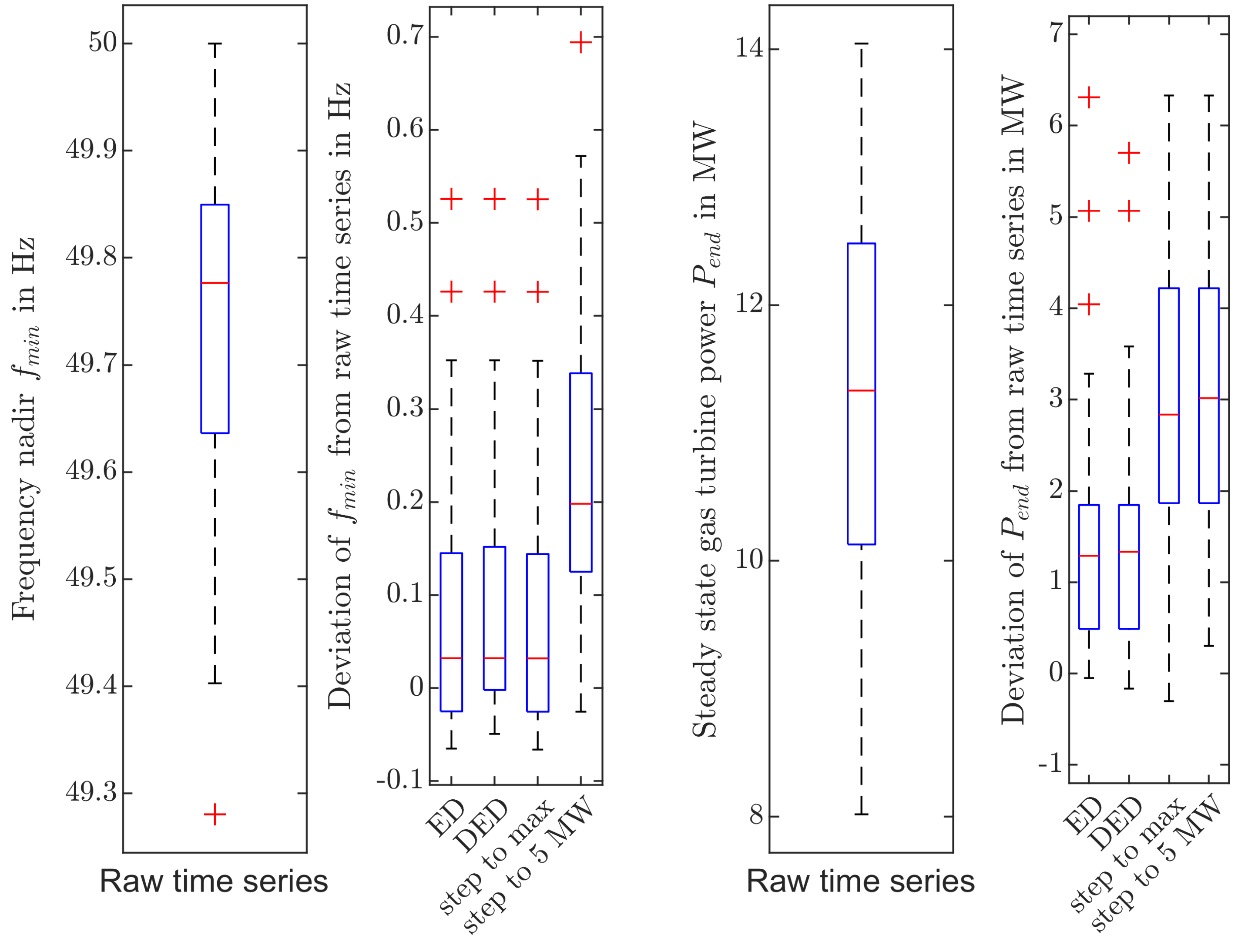
Figure 13 shows the distribution of frequency nadir and steady-state gas turbine power in the results of the 31 simulation runs using the recorded current time series as well as the deviation of and between the simulation results using the different models and the results obtained by using the recorded current time series data.
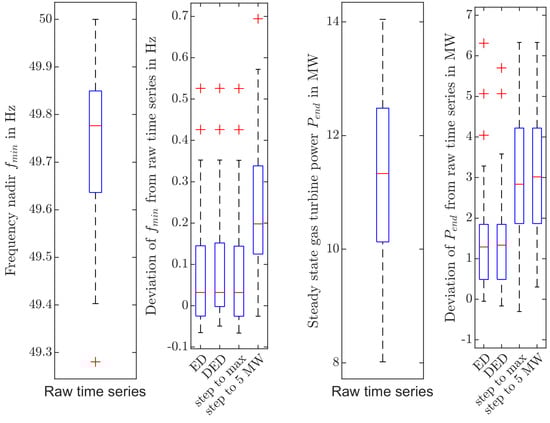
Figure 13.
Distribution of fitted model parameters: Red crosses are outliers beyond 1.5 time the interquartile range. Distribution of frequency nadir and deviation of frequency nadir and steady-state power in recorded time series and respective deviation using ED or DED CLPU models or approximating load steps to the steady-state value of 5 MW or the maximal value MW, respectively.
The RMSE is calculated as:
where N is the number of simulation runs, X is the respective results variable (power or frequency), is the result for the variable X for the nth event simulated using the recorded current time series. is the result for the variable X for the nth event simulated using the respective load model. can be fit-ED for the ED model, fit-DED for the DED model, step-max for an active power step to the fitted initial load value and step-steady for an active power step to the steady-state power value.
It can be seen that the frequency nadir is mostly determined by the initial active power step and is, therefore, equally well represented by the CLPU models and a load step to the initial active power. However, the steady-state power and frequency are better matched by simulations using the exponential decay models than either of the active power steps. Furthermore, the standard deviation among the results using the recorded current time series is in the same order of magnitude as the RMSE of the results obtained using the exponential decay models with respect to the recorded current time series. Therefore, the influence of model selection is on the same order of magnitude as the influence of event selection when considering only a single event.
The steady state values and (Table 3) are nearly identical for the different step-wise load connections of 5 MW and , respectively. This corresponds to the result shown in Figure 10 that additional load is almost completely covered by the renewable generation when it is connected step-wise without a subsequent load reduction.
As can be seen in Figure 13, all the simplified models tend to overestimate the frequency nadir (i.e., underestimate the severity of the frequency drop) as well as the steady-state power of the synchronous machine. However, using the ED and DED model yields a better representation of the distribution of than either of the step-wise power changes. Therefore, such models are more appropriate to reflect the effect of CLPU on this critical quantity during power system restoration.
The difference between the ED and the DED model are mostly negligible. Therefore, with the current amount of available measurements, no significant gain can be expected from determining an additional parameter via the DED model for the investigated scenario.
7. Discussion and Outlook
When studying power system restoration, uncertainty about the behaviour of reconnected loads should be considered. Whereas the frequency nadir after load connection can be reflected by just considering the range of expected initial consumption, other phenomena—such as the load sharing among generation units—cannot be covered by any range of mere load steps. Therefore, exponential decay models of CLPU or recorded time series data should be used when results with respect to load sharing are relevant.
The example in Section 6.2 demonstrates the challenge that CLPU can pose to active power sharing schemes among different types of generation. Furthermore, the investigation in this paper has shown that the active power sharing approach for the integration of renewable generations such as PV and wind plants introduced in [12] is rather robust concerning the range of CLPU behaviours seen in the available data, as shown in Section 6.3. However, in contrast to the power plant, where the position of the droop curve is specified by the grid operator via the setpoint, the position of the droop curve of the renewable generation results from the value of the active power that is applied when the limit value of 50.2 Hertz is exceeded. If these plants do not obtain an active power setpoint but follow available power when frequency is below 50.2 Hertz, possible frequency fluctuations around 50.2 Hertz result in the renewable generation plants feeding-in the maximum possible active power in a stationary manner. In practice, this means that the connected load is completely supplied by these plants when balancing effects have subsided if their available power permits this. This must be taken into account when performing network restoration.
Whereas delayed exponential decay of active power consumption is physically plausible and provides a slightly better fit to some recorded results, the ED model, featuring only an initial overshoot and a decay time, yields very similar results for the scenario investigated in this paper.
However, with respect to a changing load composition, in particular a higher penetration of charging an heating systems, a wide range of possible CLPU values should be considered and the development should be carefully monitored. With respect to a higher penetration of heat pumps and electric vehicle charging, the additional delay parameter of the DED model might be more relevant in the future.
Furthermore, since long-lasting outages are rare and reconnection often happens in a changed switching status, there is insufficient data to adequately cover load behaviour after such events. Therefore, it is advisable to consider a larger range of parameters in restoration studies and also to collect data and conduct further investigations whenever the opportunity arises.
Regulatory Approaches to Reduce CLPU
In order to avoid severe CLPU effects, load behaviour could be changed in one or more of the following ways: For charging of batteries as well as heating applications, power consumption after an outage could be limited for a certain time or to some upper gradient of power increase after reconnection. For load with a technical minimal load that cannot deterministically respect power consumption limits, a random delay after restoration of supply would yield similar aggregated effects. This would be in line with the connection and ramp-up limitations for distributed generation, which also requires a gradual active power increase and allows random time delays as an alternative for types of small generation units that cannot control their active power [34].
Author Contributions
C.H.: Conceptualization, methodology, simulation model for renewables and load, data analysis, visualization, discussion and writing. H.B.: simulation model of grid and gas turbine plant, visualization, review and discussion. M.B.: Discussion and review. All authors have read and agreed to the published version of the manuscript.
Funding
This research received no external funding.
Data Availability Statement
For the 31 outage events, a table of outage durations and fitted parameters for the ED, as well as the DED model, along with a matrix of simulation results and the normalized raw time series data of the events are available at https://www.uni-kassel.de/eecs/en/sections/energiemanagement-und-betrieb-elektrischer-netze/software (accessed on 29 September 2022).
Conflicts of Interest
The authors declare no conflict of interest. The funders had no role in the design of the study; in the collection, analyses, or interpretation of data; in the writing of the manuscript, or in the decision to publish the results.
Abbreviations
The following abbreviations are used in this manuscript:
| AVR | Automatik Voltage Regulator |
| BSU | Blackstart Unit |
| CLPU | Cold Load Pickup |
| ED | Exponential Decay |
| DED | Delayed Exponential Decay |
| OHL | Overhead Line |
| PLL | Phase-Locked Loop |
| PV | Photovoltaic |
| RMS | Root Mean Square |
| RMSE | Root Mean Square Error |
References
- McDonald, J.E.; Bruning, A.M. Cold Load Pickup. IEEE Trans. Power Appar. Syst. 1979, PAS-98, 1384–1386. [Google Scholar] [CrossRef]
- Friend, F. Cold load pickup issues. In Proceedings of the 2009 62nd Annual Conference for Protective Relay Engineers, College Station, TX, USA, 30 March–2 April 2009; pp. 176–187. [Google Scholar] [CrossRef]
- Kumar, I.B.; Singh, R. Measurement of Cold Load Pickup—A Case Study. IJSRD Int. J. Sci. Res. Dev. 2015, 3, 2454–2456. [Google Scholar]
- Gonzalez, M.; Wheeler, K.A.; Faried, S.O. An Overview of Cold Load Pickup Modeling for Distribution System Planning. In Proceedings of the 2021 IEEE Electrical Power and Energy Conference (EPEC), Toronto, ON, Canada, 22–31 October 2021; pp. 328–333. [Google Scholar] [CrossRef]
- IEEE Restoration Dynamics Task Force. Power System Restoration Dynamics (Issues, Techniques, Planning, Training & Special Considerations), Technical Report, PES-TPC2. 2014. Available online: https://resourcecenter.ieee-pes.org/publications/technical-reports/PESTPC2.html (accessed on 28 September 2015).
- Agneholm, E. Cold Load Pick-Up. Ph.D. Dissertation, Department of Electric Power Engineering, Chalmers University of Technology, Goeteborg, Sweden, 1999. [Google Scholar]
- Raoofsheibani, D.; Hinkel, P.; Ostermann, M.; Wellssow, W.H.; Nemati, M.; Neisius, H.T. Optimal restoration of distribution systems with active participation of volatile renewable generators. In Proceedings of the 2017 IEEE Manchester PowerTech, Manchester, UK, 18–22 June 2017; pp. 1–6. [Google Scholar]
- Hachmann, C.; Lammert, G.; Hamann, L.; Braun, M. Cold load pickup model parameters based on measurements in distribution systems. IET Gener. Transm. Distrib. 2019, 13, 5387–5395. [Google Scholar] [CrossRef]
- Braun, M.; Brombach, J.; Hachmann, C.; Lafferte, D.; Klingmann, A.; Heckmann, W.; Welck, F.; Lohmeier, D.; Becker, H. The Future of Power System Restoration: Using Distributed Energy Resources as a Force to Get Back Online. IEEE Power Energy Mag. 2018, 16, 30–41. [Google Scholar] [CrossRef]
- Papasani, A.; Zia, K.; Lee, W.J. Automatic Power System Restoration With Inrush Current Estimation for Industrial Facility. IEEE Trans. Ind. Appl. 2021, 57, 5772–5781. [Google Scholar] [CrossRef]
- Ospina, L.D.P.; Correa, A.F.; Lammert, G. Implementation and validation of the Nordic test system in DIgSILENT PowerFactory. In Proceedings of the 2017 IEEE Manchester PowerTech, Manchester, UK, 18–22 June 2017; pp. 1–6. [Google Scholar] [CrossRef]
- Hachmann, C.; Becker, H.; Theimer, F.; Thiel, P.; Braun, M. Local Power System Restoration and Islanded Operation with Combined Heat and Power Plants and Integration of Wind Power. In Proceedings of the ETG Congress 2021, Online, 18–19 March 2021; pp. 1–6. [Google Scholar]
- Lang, W.W.; Anderson, M.D.; Fannin, D.R. An Analytical Method for Quantifying the Electrical Space Heating Component of a Cold Load Pickup. IEEE Power Eng. Rev. 1981, ER-2, 38. [Google Scholar] [CrossRef]
- Benato, R.; Dambone Sessa, S.; Sanniti, F. Lessons Learnt from Modelling and Simulating the Bottom-Up Power System Restoration Processes. Energies 2022, 15, 4145. [Google Scholar] [CrossRef]
- Becker, H.; Schütt, J.; Schürmann, G.; Spanel, U.; Holicki, L.; Malekian, K. Opportunities to support the restoration of electrical grids with little numbers of large power plants through converter-connected generation and storages. IET Renew. Power Gener. 2022, 1–11. [Google Scholar] [CrossRef]
- Rodriguez Medina, D.; Rappold, E.; Sanchez, O.; Luo, X.; Rivera Rodriguez, S.R.; Wu, D.; Jiang, J.N. Fast Assessment of Frequency Response of Cold Load Pickup in Power System Restoration. IEEE Trans. Power Syst. 2016, 31, 3249–3256. [Google Scholar] [CrossRef]
- Hinkel, P.; Henschel, D.; Zugck, M.; Wellssow, W.; Torabi, E.; Guo, Y.; Rossa-Weber, G.; Gawlik, W.; Traxler, E.; Fiedler, L.; et al. Control Center Interfaces and Tools for Power System Restoration. In Proceedings of the International ETG-Congress 2019: ETG Symposium, Esslingen, Germany, 8–9 May 2019; pp. 1–6. [Google Scholar]
- Marchgraber, J.; Gawlik, W. Investigation of Black-Starting and Islanding Capabilities of a Battery Energy Storage System Supplying a Microgrid Consisting of Wind Turbines, Impedance- and Motor-Loads. Energies 2020, 13, 5170. [Google Scholar] [CrossRef]
- Agneholm, E.; Daalder, J. Cold load pick-up of residential load. IEE Proc. Gener. Transm. Distrib. 2000, 147, 44–50. [Google Scholar] [CrossRef]
- Raoofsheibani, D.; Hinkel, P.; Ostermann, M.; Roehrenbeck, S.; Wellssow, W.H. Residual load models for power system restoration: High shares of residential thermal loads and volatile PV generators. In Proceedings of the 2017 IEEE International Conference on Smart Grid Communications (SmartGridComm), Dresden, Germany, 23–26 October 2017; pp. 223–228. [Google Scholar] [CrossRef]
- Widiputra, V.; Jung, J. Development of Restoration Algorithm under Cold Load Pickup Condition using Tabu Search in Distribution System. In Proceedings of the 2018 IEEE Power Energy Society General Meeting (PESGM), Portland, OR, USA, 5–10 August 2018; pp. 1–5. [Google Scholar] [CrossRef]
- Ihara, S.; Schweppe, F.C. Physically Based Modeling of Cold Load Pickup. IEEE Trans. Power Appar. Syst. 1981, PAS-100, 4142–4150. [Google Scholar] [CrossRef]
- Nehrir, M.; Dolan, P.; Gerez, V.; Jameson, W. Development and validation of a physically-based computer model for predicting winter electric heating loads. IEEE Trans. Power Syst. 1995, 10, 266–272. [Google Scholar] [CrossRef]
- Laurent, J.; Malhame, R. A physically-based computer model of aggregate electric water heating loads. IEEE Trans. Power Syst. 1994, 9, 1209–1217. [Google Scholar] [CrossRef]
- Song, M.; nejad, R.R.; Sun, W. Robust Distribution System Load Restoration With Time-Dependent Cold Load Pickup. IEEE Trans. Power Syst. 2021, 36, 3204–3215. [Google Scholar] [CrossRef]
- Fan, R.; Sun, R.; Liu, Y. A Reduction Approach for Load Pickup Amount Considering Thermostatically Controlled Loads. In Proceedings of the 2021 IEEE Sustainable Power and Energy Conference (iSPEC), Nanjing, China, 23–25 December 2021; pp. 1634–1638. [Google Scholar] [CrossRef]
- NEW Netz GmbH. Household Load Profile. 2016. Available online: https://www.new-netz-gmbh.de/energie-marktpartner/veroeffentlichungspflichten/stromnzv/standardlastprofile (accessed on 1 December 2016).
- Renner, H.; Stadler, S.A.; Wakolbinger, C. Cold Load Pickup; TU Graz: Graz, Austria, 2013. [Google Scholar]
- IEEE Power and Energy Society. IEEE Recommended Practice for Excitation System Models for Power System Stability Studies; Technical Report. 2016. Available online: https://ieeexplore.ieee.org/document/7553421 (accessed on 1 December 2016).
- Cigre. Technical Brochure of Modeling of Gas Turbines and Steam Turbines in Combined Cycle Power Plants; Technical Report, Task Force C4.02.25. 2003. Available online: https://e-cigre.org/publication/238-modeling-of-gas-turbines-and-steam-turbines-in-combined-cycle-power-plants (accessed on 1 December 2016).
- Lammert, G.; Klingmann, A.; Hachmann, C.; Lafferte, D.; Becker, H.; Paschedag, T.; Heckmann, W.; Braun, M. Modelling of Active Distribution Networks for Power System Restoration Studies. In Proceedings of the 10th IFAC Symposium on Control of Power and Energy Systems, Tokyo, Japan, 4–6 September 2018. [Google Scholar]
- Western Electricity Coordinating Council (WECC) Renewable Energy Modeling Task Force. WECC Solar PV Dynamic Model Specification. 2012. Available online: https://www.wecc.biz/Reliability/WECC%20Solar%20PV%20Dynamic%20Model%20Specification%20-%20September%202012.pdf (accessed on 10 November 2015).
- VDE-AR-N 4120-2018-11; Technische Regeln für den Anschluss von Kundenanlagen an das Hochspannungsnetz und deren Betrieb (Technical Requirements for the Connection and Operation of Customer Installations to the High Voltage Network). VDE Verlag GmbH: Berlin/Offenbach, Germany, 2018.
- VDE-AR-N 4105; Erzeugungsanlagen am Niederspannungsnetz (Guideline for the Connection and Parallel Operation of Generation Units at Low Voltage Level). VDE Verlag GmbH: Berlin/Offenbach, Germany, 2018.
- VDE-AR-N 4110; Technische Anschlussregel Mittelspannung (Guideline for the Connection and Parallel Operation of Generation Units at Medium Voltage Level). VDE Verlag GmbH: Berlin/Offenbach, Germany, 2022.
- Van Cutsem, T.; Vournas, C. Voltage Stability of Electric Power Systems; Springer Science & Business Media: Berlin/Heidelberg, Germany, 2008. [Google Scholar]

Publisher’s Note: MDPI stays neutral with regard to jurisdictional claims in published maps and institutional affiliations. |
© 2022 by the authors. Licensee MDPI, Basel, Switzerland. This article is an open access article distributed under the terms and conditions of the Creative Commons Attribution (CC BY) license (https://creativecommons.org/licenses/by/4.0/).