Abstract
With the completion of the Lianghekou Reservoir, with a multiyear regulation capacity, the operation relationship of the cascade reservoirs in the Yalong River is becoming increasingly complex. In order to study an optimal operation mode of the cascade reservoirs in the Yalong River under different inflow frequencies, based on the shortcomings of the existing single reservoir operation mode and the local joint operation mode of the cascade reservoirs, this paper first proposed a global joint operation mode for the cascade reservoirs to develop the power generation potential of daily regulating reservoirs and then gave a solution method for the cascade reservoirs’ operational model based on an improved stochastic fractal search (ISFS) algorithm. Finally, taking the maximum power generation as the goal and the inflow data of five typical years as the model inputs, this paper analyzed the differences in the power generation and water abandonment results of the cascade reservoirs in the middle and lower reaches of the Yalong River under the above three operation modes. The results show that (1) compared with the stochastic fractal search (SFS) algorithm and the particle swarm optimization (PSO) algorithm, the ISFS algorithm had faster convergence speed and higher precision; (2) the global joint operation mode had a more significant optimization effect in the year with more inflow, followed by the local joint operation mode, and the single reservoir operation mode had the worst; however, the difference in the results of the three operation modes gradually decreased as the inflows gradually decreased.
1. Introduction
China is the country with the most abundant water resources in the world, and hydropower plays an important role in adjusting China’s energy structure, reducing greenhouse gas emissions and addressing climate change [1]. As the third largest hydropower base in China, the main development task of the Yalong River is power generation. The difference in the inflow between the dry season and the flood season of the Yalong River is obvious, and it seriously affects the power generation benefit of the reservoir. Therefore, it is necessary to build large reservoirs with a good regulating capacity to reasonably regulate and distribute the annual runoff [2].
With the construction and operation of large-scale cascade reservoirs in the lower reaches of the Yalong River, a relationship of the water volume and water head between the upstream and downstream reservoirs has gradually formed [3]. The traditional single reservoir operation method has not been able to meet the needs of the joint operation of the cascade reservoirs [4,5]. The joint operation of the cascade reservoirs is an important way to realize the rational distribution and efficient utilization of water resources [6,7]. Since the dynamic programming (DP) method was proposed in the 1960s, various optimization methods have been continuously applied to solve the problem of an optimal operation strategy of the cascade reservoirs. For example, Chen et al. [8] and Huang et al. [9] applied the DP and progressive optimization (POA) algorithms to the long-term power generation optimization operation of the Jinxi Reservoir and Ertan Reservoir, respectively. Ji et al. [10] applied multistage dynamic programming (MSDP) to the short-term optimization operation of the Jinxi Reservoir and the Guandi Reservoir. Chen et al. [11] applied the multistep progressive optimization algorithm (MSPOA) to the operation of the gate and the optimal flow of the cascade reservoirs in the lower reaches of the Yalong River. Zhang et al. [12] proposed an improved progressive optimization algorithm (IPOA) by combining the POA algorithm with the spatial mapping principle and applied it to the short-term operational optimization model of the cascade reservoirs in the lower reaches of the Yalong River considering the effect of water flow hysteresis. The study showed that the above traditional optimization methods have a dimensional disaster problem in solving the operational model problem of large-scale cascade reservoirs [13]. With the development of computer technology in the 21st century, various intelligent optimization algorithms have gradually been used in the optimal operation of the Yalong River cascade reservoirs. For example, Xiong et al. [14] applied the genetic algorithm (GA) to the flood-control operation of the Jinxi Reservoir and the Ertan Reservoir. Chen et al. [15] proposed an adaptive multivariable strategy particle swarm optimization algorithm based on the uniform mutation operation of nonoptimal particles and applied it to the cascade reservoir operation in the lower reaches of the Yalong River. Han et al. [16] proposed an adaptive genetic algorithm to obtain the optimal operation rules of the Jinxi Reservoir and the Jindong Reservoir considering the ecological flow. Wang et al. [17] took the Jinxi Reservoir and the Guandi Reservoir as examples and applied the proposed extreme value theory genetic algorithm to short-term power generation planning under different runoff prediction errors.
It can be seen from previous studies that the operational range of the Yalong River cascade reservoirs is mostly from the Jinxi Reservoir to the Tongzilin Reservoir in the downstream. With the completion and operation of the Lianghekou Reservoir with a multiyear regulation capacity in the middle reaches of the Yalong River, the inflow of the downstream reservoirs will be greatly affected [18]; thus, it is necessary to study the optimal operation mode of the Yalong River cascade reservoirs including the Lianghekou Reservoir. Since the cascade reservoirs of the Yalong River are a complex operational system, including multiyear regulation, annual regulation, seasonal regulation and daily regulation, most of the current studies take the water level of the daily regulating reservoir as a fixed value and only optimize the flow process of the Lianghekou Reservoir, Jinxi Reservoir and Ertan Reservoir with good regulating performance [19,20,21]. However, this local joint operation mode of the cascade reservoirs ignores the power generation potential of the daily regulating reservoirs. Therefore, it is necessary to study the global joint operation mode of the cascade reservoirs including the daily regulating reservoirs.
With the increase in the number of cascade reservoirs in the Yalong River, the operational relationship between reservoirs with different regulating capacities becomes more complex. The joint operation of the cascade reservoirs is a multiconstrained, nonlinear and high-dimensional problem [22]. In addition to exploring the appropriate operation mode, it is crucial to choose an efficient solution method [23]. Inspired by the random growth process in nature and the mathematical concept of fractals, Hamid Salimi, a scholar at the University of Tehran in Iran, proposed the stochastic fractal search (SFS) algorithm in 2015 [24]. The SFS algorithm is widely used in various engineering optimization problems because of its better global search capability [25,26,27], but it is currently less often used in reservoir operation [28]. Studies have shown that the SFS algorithm has shortcomings such as slow convergence speed and low optimization accuracy when solving complex functions [29,30]. To improve the optimization capability of the SFS algorithm in the cascade reservoirs’ operational model, inspired by the optimization mechanism of the PSO algorithm, this study proposed the improved stochastic fractal search (ISFS) algorithm and applied it to three modes: single reservoir operation, local joint operation of cascade reservoirs and global joint operation of the cascade reservoirs. In order to study the optimal operation mode of the cascade reservoirs in the Yalong River under different inflow frequencies, this study used the inflow data of five typical years as model inputs.
The remainder of this study is organized as follows: Section 2 describes the cascade reservoirs’ operational optimization model including the single reservoir operational optimization model and the cascade reservoirs’ joint operational optimization model. Section 3 introduces the main steps of the PSO algorithm, SFS algorithm and ISFS algorithm and the model solving method based on the ISFS algorithm. Section 4 presents an overview of the study area, data processing and parameter settings. Section 5 studies and discusses the efficiency of the ISFS algorithm in solving the problem of the cascade reservoirs’ operational model and the optimal operation mode of cascade reservoirs under different inflow frequencies; Section 6 is the conclusion.
2. Cascade Reservoirs’ Operational Optimization Model
In order to formulate the optimal strategy for the cascade reservoirs’ power generation operation, firstly, the corresponding objective function should be determined according to the selected optimization criteria, and then the cascade reservoirs’ operational optimization model should be established according to the known runoff process and constraints. There are three main optimization criteria for cascade reservoir power generation operation: (1) the total power generation during the operational period is the largest; (2) the total power generation benefit is the largest; (3) the minimum output is the largest. In this study, the maximum total power generation was chosen as the objective function, and the single reservoir operational optimization model and the cascade reservoirs joint operational optimization model were developed.
2.1. Single Reservoir Operational Optimization Model
A single reservoir optimal operation means that each reservoir operates in its own most favorable way. On the basis of determining the optimal outflow of an upstream reservoir, the downstream reservoirs are optimized one by one. The total power generation of cascade reservoirs is the sum of the optimal power generation of each reservoir.
2.1.1. Objective Function
With the goal of maximizing the power generation of a single reservoir, the objective function of the single reservoir operational optimization model is shown in Equation (1):
where is the power generation of the kth hydropower station during the operational period, unit: kWh; T is the number of stages over the whole operational period; is the number of cascade hydropower stations; is the comprehensive output coefficient of the kth hydropower station; is the outflow through the turbines of the kth reservoir in the tth stage, unit: m3/s; is the average water head of the kth hydropower station in the tth stage, unit: m; is the number of operation hours of each stage, unit: h.
2.1.2. Constraints
- (1)
- The water balance constraint is shown in Equation (2):where and are the initial and final storage volumes of the kth reservoir in the tth stage, respectively, unit: m3; and are the inflow and the total outflow of the kth reservoir in the tth stage, respectively, unit: m3/s.
- (2)
- The hydraulic contact constraint is shown in Equation (3):where is the interval flow of reservoir k and k − 1 in the tth stage, unit: m3/s.
- (3)
- The water level constraints are shown in Equation (4):where and are the minimum and maximum water levels of the kth reservoir in the tth stage, respectively, unit: m.
- (4)
- The output constraints are shown in Equation (5):where and are the minimum and maximum outputs of the kth reservoir in the tth stage, respectively, unit: kW.
- (5)
- The flow constraints are shown in Equations (6) and (7):where is the lower limit of ; is the upper limit of ; is the lower limit of ; is the upper limit of .
- (6)
- The boundary conditions limits constraints are shown in Equations (8) and (9):where is the water level of the kth reservoir at the beginning of the first stage; is the water level of the kth reservoir at the beginning of the whole operational period; is the water level of the kth reservoir at the end of the Tth stage; is the water level of the kth reservoir at the end of the whole operational period.
2.2. Joint Operational Optimization Model of the Cascade Reservoirs
Taking the cascade reservoirs as a whole, the optimal outflow flow of all reservoirs was determined at the same time, and the power generation could be maximized through the regulation capacity of the cascade reservoirs.
2.2.1. Objective Function
Aiming at maximizing the total power generation of cascade reservoirs, the objective function of the joint operational optimization model of cascade reservoirs is shown in Equation (10):
where is the total power generation of the cascade reservoirs during the operational period, unit: kWh.
2.2.2. Constraints
The constraints are the same as those of the single reservoir operational optimization model in Section 2.1.2.
2.3. Constraints Handling Strategy
The cascade reservoirs’ operational optimization model mainly includes three constraints: water level, flow and output, which can be transformed into each other through the hydraulic connection between reservoirs. This study used the water level as the decision variable and the water level corridor method to deal with the above constraints. Firstly, the dead water level and normal water level of each reservoir were taken as the initial water level constraint interval. Then, based on the water balance equation and the characteristic curves related to the reservoir, the flow constraints and output constraints were transformed into the corresponding water level interval one by one. Finally, the intersection of the above water level intervals was taken to obtain the feasible water level interval of each operational stage. During the optimization, when the water level exceeded the boundary of the corridor, it was corrected to the boundary value. This method makes the complex constraints handling simpler and more intuitive.
3. Model Solving Based on the ISFS Algorithm
3.1. PSO Algorithm
James Kennedy and Russell Ebethart, in the United States, proposed the PSO algorithm in 1995, which was inspired by the foraging behavior of bird flocks [31]. As a representative of swarm intelligence, the PSO algorithm is widely used in various optimization problems due to the fact of its high optimization efficiency [32]. The feasible solution for each optimization problem is a particle, and the velocity of particle i in d-dimensional space determines its flying direction and distance. The position of particle i is denoted as , and then the population updates its velocity and position by dynamically tracking two extreme points. The first one is the optimal solution found by the particle itself in the iterative process, called the individual extreme point = (,,…,), and the other one is the optimal solution found by the population in the iterative process, called the global extreme point = (,,…,). The particle updates its velocity and position according to Equations (11) and (12):
where k is the number of iterations; w is the inertia weight; and are acceleration factors; and are random numbers in [0,1]. The parameter w controls the effect of the speed of the previous iteration on the speed of the current iteration [33]. A larger value for w facilitates the search for a global optimal solution, while a lower value for w facilitates the local search in the current region. A strategy incorporating inertia weights w is proposed in [34]. A suitable and can increase the convergence speed and do not easily fall into local optimum; and are usually taken to be equal to 2 [35]. The velocity of the particle cannot exceed the maximum velocity [36].
3.2. SFS Algorithm
The SFS algorithm mainly includes a diffusion process and two update processes [24].
- (1)
- Diffusion process
After initializing all individuals, each individual diffuses around the current position until a predetermined maximum number of diffusions is reached [37], which increases the chance of finding the global optimum and prevents getting trapped in a local optimum [38]. In order to effectively avoid a sharp increase in the number of individuals during the diffusion process, the best individuals are the only ones that are retained, and the rest are discarded. The Gaussian wander involved in the diffusion process is shown in Equation (13):
where and are random numbers in [0,1]; and are the positions of the best individual and individual i in the population, respectively. The calculated value of standard deviation, , is shown in Equation (14), where g is the current number of iterations:
- (2)
- First update process
After the diffusion process, the value of the fitness function of the individual is first ranked, and then the individual is assigned a probability, , according to Equation (15). If the individual satisfies the condition , the position of the individual is updated according to Equation (16), where is the new position of ; otherwise, the position of the individual remains unchanged. The first update process can be expressed as:
where N is the number of individuals in the population; and are randomly selected individuals from the population.
- (3)
- Second update process
As in the first update process, if the individual satisfies the condition , the current position of is updated according to Equations (17) and (18), where is the new position of ; otherwise, the position of is kept unchanged. The new individual replaces if its fitness function value is better than . The two ways of the second update process are as follows:
where and are randomly selected individuals from the population; is a random number generated from a Gaussian normal distribution.
3.3. ISFS Algorithm
In order to further improve the convergence speed and accuracy of the SFS algorithm in the optimization process, inspired by the search strategy of the PSO algorithm, the ISFS algorithm proposed in this study uses the global extreme point, gbest, and the individual extreme point, pbest, to guide the individual in the second update process. However, it is shown that the vector difference between individuals gradually decreases in the process of chasing the current optimal solution, so that individuals cannot evolve and fall into the local optimal point [39]. To avoid the ISFS algorithm from falling into a local optimum during the optimization process, this study used the adaptive variation rate to control the rate at which individuals move toward the optimal point. The variation rate is taken as a small value at the beginning of the iteration to guide individuals towards the optimal point. The variation rate was taken as an increasing value during the iteration to increase the possibility of the algorithm jumping out of the local optimal point [40]. The flow of the ISFS algorithm is shown in Figure 1.
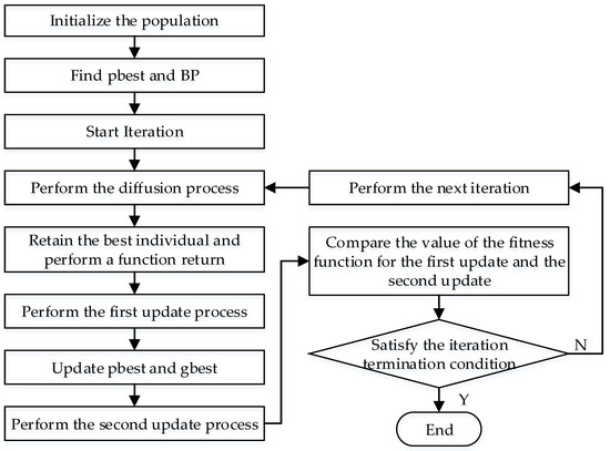
Figure 1.
The flowchart of the ISFS algorithm.
Step 1: Let the iteration number be g = 1 and initialize the population including the population size (sizepop), the spatial dimensions of the individual (dim) and the initial position ();
Step 2: Calculate the values of the fitness function for all individuals and find the optimal individual BP;
Step 3: Set the diffusion number of the individuals and perform the diffusion process. The current individual position is diffused according to Equations (13) and (14), and the value of the fitness function of the best individual is returned;
Step 4: Perform the first update process. The corresponding probability value, , of the individual is obtained according to Equation (15). If the individual satisfies the condition , then the position of the new individual is obtained according to Equation (16); otherwise, the position of the individual remains unchanged. Calculate the fitness function values for all individuals and update the positions of the individual extreme value points, , and global extreme value points, ;
Step 5: Perform the second update process. If the individual satisfies the condition , the position of the new individual is obtained according to Equation (19); otherwise, the position of is kept unchanged. The adaptive variation rate is calculated as shown in Equation (20), where and are the lower and upper limits of the variation rate, respectively.
Step 6: Let g = g + 1. If the maximum number of iterations is reached, the algorithm ends; otherwise, return to Step 2.
3.4. Procedure for Solving the Optimal Operation Strategy Using the ISFS Algorithm
The single reservoir operational optimization model takes the water level of each reservoir at the end of the operational stage as the decision variable, and the cascade reservoir operational optimization model takes the water levels of all reservoirs at the end of the same operational stage as the decision variable. When the ISFS algorithm is used to solve the problem of the cascade reservoirs’ operational optimization model, the individual is given a specific meaning, which is a feasible water level process in the operational period. The spatial dimensions of an individual is defined as the product of the number of reservoirs N and the total number of operational stages T. The procedure for solving the problem of the optimal operation strategy using the ISFS algorithm is shown in Figure 2.
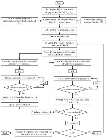
Figure 2.
Flowchart of the procedure for solving the problem of the optimal operation strategy using the ISFS algorithm.
Step 1: Let the iteration number be g = 1, set the population size (sizepop), the maximum number of iterations (G) and the algorithm parameters ( and );
Step 2: Randomly generate the initial population according to Equation (21), where is the water level at the end of the jth stage; and are the upper and lower boundaries of the water level obtained according to the operational model and constraint handling strategy in Section 2; is random number in [0,1].
Step 3: Calculate the objective function value corresponding to each water level process, and find the water level process BP that maximizes the objective function value;
Step 4: The same as Step 3 to Step 5 in the ISFS algorithm, the diffusion process, the first update process and the second update process are executed separately for the population, and the water level beyond the boundary after each change is corrected;
Step 5: Let g = g + 1. If the maximum number of iterations is reached, then output the optimal power generation and water level process, etc.; otherwise, return to Step 3 to continue the iterative calculation.
4. Case Study
4.1. Study Area
The cascade reservoirs in the middle and lower reaches of the Yalong River were taken as the case study. The Yalong River is the largest tributary of the Jinsha River in western Sichuan Province, China, with a total length of 1571 km, a natural drop of 3830 m and an annual runoff of 60.9 billion m3. At present, seven reservoirs have been built in the middle and lower reaches of the Yalong River, namely, Lianghekou (LHK), Yangfanggou (YFG), Jinxi (JX), Jindong (JD), Guandi (GD), Ertan (ET) and Tongzilin (TZL), with a total installed capacity of 19,200 MW. The location and characteristic parameters of the cascade reservoirs in the Yalong River Basin are shown in Figure 3 and Table 1, respectively. The Lianghekou Reservoir and Yangfanggou Reservoir in the middle reaches of the Yalong River were completed in September 2021 and November 2021, respectively. The Lianghekou Reservoir, with a multiyear regulation capacity, is the control reservoir in the middle and lower reaches of the Yalong River; therefore, its operation mode has a great influence on the power generation benefit of downstream cascade reservoirs. The Jinxi Reservoir to the Tongzilin Reservoir in the lower reaches of the Yalong River have been fully developed since 2015, among which the Jinxi Reservoir has an annual regulation capacity and Ertan Reservoir has a seasonal regulation capacity. The other four reservoirs are daily regulating reservoirs. With a total regulating capacity of 14.84 billion m3, the Lianghekou Reservoir, Jinxi Reservoir and Ertan Reservoir have an extremely strong runoff regulating capacity, making the Yalong River the only large river in China managed by one owner. In addition, the cascade reservoirs of the Yalong River with a multiyear regulation capacity will also have a positive impact on water resource allocation in the middle and lower reaches of the Yangtze River, reducing the flood risk of the Three Gorges Reservoir and Gezhouba Reservoir in the flood season.

Figure 3.
Location of the cascade reservoirs in the Yalong River Basin.

Table 1.
Characteristic parameters of the Yalong River cascade reservoirs.
4.2. Data Processing and Parameter Settings
The flood season in the Yalong River Basin lasts from June to November, and the dry season lasts from December to May of the following year. The reservoir reaches its dead level at the beginning of June; thus, the hydrological year of the basin is set to run from June to May. This study took the hydrological year of the Yalong River Basin as the operational period and ten days as an operational stage. In the single reservoir operation mode, the initial and final water levels of each reservoir in the operational period were set as the dead water level, and the cascade reservoirs were optimized one by one. The Yangfanggou Reservoir, Jindong Reservoir, Guandi Reservoir and Tongzilin Reservoir belong to daily regulating reservoirs with small regulating storage capacities and poor water storage capacities. In the local joint operation mode of the cascade reservoirs, the initial and final water levels of the Lianghekou Reservoir, Jinxi Reservoir and Ertan Reservoir were dead levels, while the water level process of each daily regulating reservoir during the operational period was fixed as the average of the dead water level and the normal water level so that the inflow of the daily regulating reservoir was equal to the outflow. In the global joint operation mode of the cascade reservoirs proposed in this study, the water level process of the cascade reservoirs, including the daily regulating reservoirs, was optimized by setting the initial and final water levels of all reservoirs as dead water levels during the operational period.
This study selects the inflow data of five typical years as the model input, namely, the wet year (p = 10%, 2012), relatively wet year (p = 30%, 2008), normal year (p = 50%, 2015), relatively dry year (p = 70%, 2013) and dry year (p = 90%, 2006), where 2012, 2008, 2015 and 2013 were called nondrought years and 2006 was called a drought year. The ISFS algorithm, SFS algorithm and PSO algorithm were used to solve the above three operation modes, respectively. Considering the solution accuracy and calculation time of the algorithm, the population size (sizepop) and number of iterations (G) of the three algorithms were set to 100 and 500, respectively, and the individual diffusion number for the SFS algorithm and ISFS algorithm was 100. Based on the test results of the ISFS algorithm and PSO algorithm in the optimal operation of the cascade reservoirs in the Yalong River, the upper limit of variability () and the lower limit of variability () in the ISFS algorithm were 0.9 and 0.2, respectively, and the acceleration coefficients ( and ), inertia weight (w) and maximum velocity () in the PSO algorithm were 2, 2, 0.8 and 2, respectively.
5. Results and Discussion
5.1. Test of the ISFS Algorithm
In order to test the efficiency of the ISFS algorithm in solving the problem of the operational model of the cascade reservoirs, the ISFS algorithm, SFS algorithm and PSO algorithm were used to solve the single reservoir operation mode (called “Scheme 1”), the cascade reservoirs local joint operation mode (called “Scheme 2”) and the cascade reservoirs global joint operation mode (called “Scheme 3”), respectively. Considering the randomness and instability of the algorithm, each algorithm was run independently for 10 times, and the result closest to the average value of the objective function was taken as the optimal operation strategy for the cascade reservoirs.
Table 2 shows the optimization results of the three schemes obtained by applying the ISFS algorithm, SFS algorithm and PSO algorithm in five typical years. Table 3 shows the improved power generation and water resource utilization rate of the cascade reservoirs by the ISFS algorithm compared with the SFS algorithm and PSO algorithm.
Table 2.
Optimization results of the three schemes obtained by applying the ISFS algorithm, SFS algorithm and PSO algorithm in five typical years.
Table 3.
Total power generation (108 kWh) and water resource utilization rate improved by the ISFS algorithm compared with the SFS algorithm and PSO algorithm.
From the overall optimization results under the different schemes in Table 2, it can be seen that the three algorithms had better optimization results using Scheme 3 in the nondrought years and Scheme 1 in the drought year. From the optimization results of the three algorithms in Table 2 under the same scheme and inflow frequency, it can be seen that the ISFS algorithm could obtain the maximum total power generation and the smallest abandoned water. As can be seen from Table 3, due to the limited regulation capacity of a single reservoir in Scheme 1, the power generation of the five typical years and the water resource utilization of the nondrought years obtained by the ISFS algorithm were higher than those by the SFS algorithm and the PSO algorithm. While in Scheme 2 and Scheme 3, due to the larger regulation capacity of the cascade reservoirs, the power generation and water utilization rate of the cascade reservoirs obtained by the ISFS algorithm significantly increased compared with the PSO algorithm, and the increase effect was more significant compared with the SFS algorithm. Under the inflow in 2015, 2013 and 2006, the water resource utilization rate of the ISFS algorithm and the PSO algorithm in Scheme 2 and Scheme 3 reached 100%, while the SFS algorithm still had a small amount of abandoned water.
Figure 4 shows the convergence process of the three algorithms when solving Scheme 3 with the inflow data of 2008, 2015 and 2013 as the model inputs. It can be seen that the ISFS algorithm not only had a high initial value but also the largest growth rate at the beginning of the iteration so that the objective function value can converge to the approximate optimal value within 100 iterations. In contrast, the PSO algorithm had a slower growth rate and converged to an approximate optimal solution in 300 iterations, and the SFS algorithm had the slowest growth rate and easily fell into a local optimal solution.
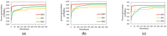
Figure 4.
Convergence process of Scheme 3 solved by the three algorithms in (a) 2008, (b) 2015 and (c) 2013.
5.2. Comparison of the Three Schemes
Then, based on the optimization results of the ISFS algorithm, the differences in the optimization results, power generation rules and outflow processes of the cascade reservoirs in the three schemes adopted in the five typical years were analyzed.
5.2.1. Optimization Results of the Cascade Reservoirs
In Table 2, the total power generation of Scheme 3 in the five typical years increased by 0.54%, 0.62%, 0.58%, 0.51% and 0.42%, respectively, compared to Scheme 2, which indicates that Scheme 3 can better utilize the regulating capacity of the cascade reservoirs; thus, Scheme 3 obtains a greater total power generation in the five typical years. The total power generation of Scheme 3 in the five typical years increased by 2.85%, 1.99%, 2.30%, 1.47%, and −0.61%, respectively, compared with Scheme 1. It can be seen that although the total power generation of Scheme 3 in the nondrought years was greater than that of Scheme 1, the difference in the power generation between the two schemes generally showed a decreasing trend with the decrease in inflow, and the total power generation of Scheme 1 in the drought years exceeded that of Scheme 3. The reason for this is that an upstream reservoir does not have excess water to recharge the downstream in a dry year, which greatly weakens the adjustment ability of Scheme 3 for cascade reservoirs.
It can be seen from Table 2 that when the inflow data of 2012 and 2008 were used as model inputs, the water resource utilization rate of Scheme 3 increased by 3.56% and 17.89%, respectively, compared with Scheme 2, and increased by 35.66% and 97.33%, respectively, compared with Scheme 1. When the inflow data of 2015 and 2013 were used as the model inputs, Scheme 2 and 3 achieved 100% water utilization, while Scheme 1 had 1.787 billion m3 and 1.148 billion m3 of abandoned water. When the inflow data in 2006 were used as the model input, the water abandonment of the three schemes was 0. This shows that Scheme 1 had the lowest water resources utilization rate in the nondrought years, while Scheme 2 and Scheme 3 could use the regulation capacity of the cascade reservoirs to allocate the water resources reasonably during the operational period, thus improving the overall water resources utilization rate, but Scheme 3 had a higher water resources utilization rate than Scheme 2.
5.2.2. Power Generation Rules of Cascade Reservoirs
Table 4 shows the power generation of each reservoir obtained by the three schemes in the five typical years. Table 5 shows that the power generation of each reservoir increased by Scheme 3 over Scheme 1. Table 6 shows that the power generation of the Lianghekou Reservoir, Jinxi Reservoir and Ertan Reservoir as well as the daily regulating reservoirs increased by Scheme 3 compared with Scheme 2.
Table 4.
Power generation (108 kWh) of each reservoir obtained by the three schemes in the five typical years.
Table 5.
Power generation (108 kWh) of each reservoir increased by Scheme 3 compared with Scheme 1.
Table 6.
Power generation (108 kWh) of the Lianghekou Reservoir, Jinxi Reservoir and Ertan Reservoir as well as the daily regulating reservoirs increased by Scheme 3 compared with Scheme 2.
From the results of the power generation in the nondrought years, as shown in Table 4 and Table 5, it can be seen that the power generation of the Lianghekou Reservoir in Scheme 1 was higher than that of Scheme 3 when the inflow data of 2012 were used as the model input, but Scheme 3 was more effective in compensating for the power generation from the Yangfanggou Reservoir to the Tongzilin Reservoir. When the inflow data of 2008, 2015 and 2013 were used as the model inputs, the power generation of the Lianghekou Reservoir and the Yangfanggou Reservoir in Scheme 1 was higher than that of Scheme 3, but Scheme 3 compensated for the power generation from the Jinxi Reservoir to the Tongzilin Reservoir. The analysis shows that Scheme 1 aimed at the maximum power generation of a single reservoir without considering the water demand of the downstream reservoirs, resulting in the power generation loss of the downstream cascade reservoirs. While Scheme 3 aimed at maximizing the power generation of the cascade reservoirs so that the power generation of the downstream reservoirs could be compensated more by the regulating capacity of the cascade reservoirs, thus improving the overall power generation of the cascade reservoirs. However, with the gradual reduction of inflow, the compensation range and compensation power generation of the downstream reservoirs in Scheme 3 were reduced. From the results of the power generation in the drought year, as shown in Table 4 and Table 5, it can be seen that when the inflow data in 2006 were used as the model input, the power generation from the Lianghekou Reservoir to the Guandi Reservoir in Scheme 3 was significantly lower than that of Scheme 1, while the power generation of the Ertan Reservoir and the Tongzilin Reservoir was higher than that of Scheme 1. The analysis shows that although the Ertan Reservoir and the Tongzilin Reservoir partially compensated for the power generation from the upstream Lianghekou Reservoir to the Guandi Reservoir, it was more advantageous to adopt Scheme 1 in the drought year.
As can be seen from Table 4 and Table 6, the total power generation of the Lianghekou Reservoir, Jinxi Reservoir and Ertan Reservoir in Scheme 2 and Scheme 3 did not differ significantly in the five typical years, but the power generation compensation of Scheme 3 to the Jindong Reservoir, Guandi Reservoir and Tongzilin Reservoir in the downstream was more obvious. The analysis shows that although Scheme 2 and Scheme 3 could utilize the regulating capacity of the Lianghekou Reservoir, Jinxi Reservoir and Ertan Reservoir to improve the overall power generation of the cascade reservoirs, Scheme 3 could better optimize the flow process of the daily regulating reservoirs.
5.2.3. Outflow Process of the Cascade Reservoirs
Figure 5, Figure 6, Figure 7, Figure 8, Figure 9, Figure 10 and Figure 11 show the water levels and flow processes of the cascade reservoirs obtained by the three schemes under the inflow of 2008. In order to make the water level of the cascade reservoirs drop to the dead water level at the end of the operational period, Scheme 1 significantly increased the outflow of the cascade reservoirs in April, resulting in a large amount of abandoned water in the Jindong Reservoir and the Ertan Reservoir during the dry season, while Schemes 2 and 3 increased the outflow of the cascade reservoirs from February so that no water abandonment occurred in the dry season. Compared with Scheme 1, Scheme 2 and Scheme 3 both improved the water resource utilization rate and output of the cascade reservoirs during the dry season. Compared with Scheme 2, the water resource utilization rate and power generation of the cascade reservoirs in Scheme 3 increased by 17.89% and 670 million kWh, respectively. It can be seen that Scheme 3 could more reasonably arrange the outflow processes of the cascade reservoirs during the operational period.
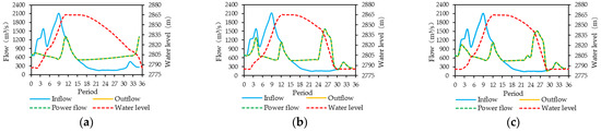
Figure 5.
Operation hydrographs of the Lianghekou Reservoir using (a) Scheme 1, (b) Scheme 2 and (c) Scheme 3.

Figure 6.
Operation hydrographs of the Yangfanggou Reservoir using (a) Scheme 1, (b) Scheme 2 and (c) Scheme 3.
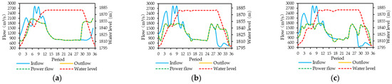
Figure 7.
Operation hydrographs of the Jinxi Reservoir using (a) Scheme 1, (b) Scheme 2 and (c) Scheme 3.

Figure 8.
Operation hydrographs of the Jindong Reservoir using (a) Scheme 1, (b) Scheme 2 and (c) Scheme 3.

Figure 9.
Operation hydrographs of the Guandi Reservoir using (a) Scheme 1, (b) Scheme 2 and (c) Scheme 3.
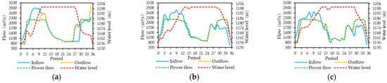
Figure 10.
Operation hydrographs of Ertan Reservoir using (a) Scheme 1, (b) Scheme 2 and (c) Scheme 3 respectively.
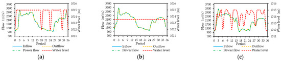
Figure 11.
Operation hydrographs of the Tongzilin Reservoir using (a) Scheme 1, (b) Scheme 2 and (c) Scheme 3.
6. Conclusions
Taking the maximum power generation of the cascade reservoirs as the objective function, the single reservoir operation mode, the local joint operational model of the cascade reservoirs and the global joint operational model of the cascade reservoirs were established and solved using the ISFS algorithm proposed in this study. On this basis, the proposed algorithm was applied to discuss the optimal operation mode of the Yalong River cascade reservoirs under five typical years. The conclusions drawn from this study are as follows:
- (1)
- Compared with the SFS algorithm and the PSO algorithm, the ISFS algorithm had the fastest convergence speed and the best optimization results in the three operation modes, and the difference in the power generation under the global joint operation mode of the cascade reservoirs was the most obvious;
- (2)
- In the years with larger inflow, the optimization effect of the global joint operation mode was more obvious for cascade reservoirs in the Yalong River. Compared with the single reservoir operation mode, the local joint operation mode and the global operation mode could utilize the regulating storage capacity of the cascade reservoirs to reasonably allocate the water resources of the downstream Jinxi Reservoir to the Tongzilin Reservoir, thereby significantly increasing the power generation and water resource utilization of the cascade reservoirs, but the latter had a more significant optimization effect on the downstream daily regulating reservoirs;
- (3)
- In the years with smaller inflow, the difference among the results of the three operation modes for the cascade reservoirs on the Yalong River was smaller. As the water supply of the upstream reservoirs to the downstream reservoirs gradually decreased, the regulation ability of the cascade reservoirs weakened, and the compensation range and compensation power generation of the global joint operation mode to the downstream reservoirs were reduced. In the drought year of p = 90%, the total power generation of a single reservoir operation mode eventually exceeded that of the global joint operation mode.
The ISFS algorithm proposed in this study effectively avoids the problem that the SFS algorithm easily falls into the local optimal value and provides a new optimization method for the cascade reservoirs’ operational model. In addition, this study also provides a reference for the operation mode selection of complex cascade reservoir systems including daily regulating reservoirs under different inflow frequencies. It should be noted that the global joint operation mode of the cascade reservoirs proposed in the study aimed at maximizing the overall interests of the cascade reservoirs. This method is only applicable to cascade reservoirs under the management of the same owner. When cascade reservoirs are managed by different owners, the global joint operation mode of the cascade reservoirs is often difficult to carry out due to the presence of conflicts of interests. Therefore, in future research, it is urgent to study the operation mode of inter-basin cascade reservoirs with different owners.
Author Contributions
Conceptualization, A.X. and Q.W.; methodology, A.X.; software, A.X.; validation, L.M.; data curation, L.M.; writing—original draft preparation, A.X.; writing—review and editing, A.X.; visualization, Q.W.; supervision, L.M. All authors have read and agreed to the published version of the manuscript.
Funding
This research was funded by the National Natural Science Foundation of China (No. 51979114) and the Fundamental Research Funds for the Central Universities (No. 2017KFYXJJ199).
Data Availability Statement
Not applicable.
Acknowledgments
Special thanks are given to the anonymous reviewers and editors for their constructive comments.
Conflicts of Interest
The authors declare no conflict of interest.
References
- Li, X.; Gui, F.; Li, Q. Can Hydropower Still Be Considered a Clean Energy Source? Compelling Evidence from a Middle-Sized Hydropower Station in China. Sustainability 2019, 11, 4261. [Google Scholar] [CrossRef]
- Liu, X.; Yang, M.; Meng, X.; Wen, F.; Sun, G. Assessing the Impact of Reservoir Parameters on Runoff in the Yalong River Basin using the SWAT Model. Water 2019, 11, 643. [Google Scholar] [CrossRef]
- Ehteram, M.; Karami, H.; Mousavi, S.; Farzin, S.; Kisi, O. Optimization of energy management and conversion in the multi-reservoir systems based on evolutionary algorithms. J. Clean. Prod. 2017, 168, 1132–1142. [Google Scholar] [CrossRef]
- Jiang, Z.; Liu, P.; Ji, C.; Zhang, H.; Chen, Y. Ecological flow considered multi-objective storage energy operation chart optimization of large-scale mixed reservoirs. J. Hydrol. 2019, 577, 123949. [Google Scholar] [CrossRef]
- Li, R.; Jiang, Z.; Li, A.; Yu, S.; Ji, C. An improved shuffled frog leaping algorithm and its application in the optimization of cascade reservoir operation. Hydrol. Sci. J. 2018, 63, 2020–2034. [Google Scholar] [CrossRef]
- Lu, S.; Shang, Y.; Li, W.; Peng, Y.; Wu, X. Economic benefit analysis of joint operation of cascaded reservoirs. J. Clean. Prod. 2018, 179, 731–737. [Google Scholar] [CrossRef]
- Guo, S.; Chen, J.; Li, Y.; Liu, P.; Li, T. Joint Operation of the Multi-Reservoir System of the Three Gorges and the Qingjiang Cascade Reservoirs. Energies 2011, 4, 1036–1050. [Google Scholar] [CrossRef]
- Chen, L.; Mei, Y.; Yang, N.; Wei, J. Modeling long-term optimal operation of hydropower plants using hydropower correlation matrix. Eng. J. Wuhan Univ. Eng. Ed. 2009, 42, 308–312. [Google Scholar]
- Huang, W.; Ma, G.; Wang, H.; Tang, M.; Wang, L. Study on the mid-long term optimal operation model and its algorithm for cascade hydropower stations on the lower-reach of Yalong River. J. Hydroelectr. Eng. 2009, 28, 1–4. [Google Scholar]
- Ji, C.; Li, C.; Wang, B.; Liu, M.; Wang, L. Multi-Stage Dynamic Programming Method for Short-Term Cascade Reservoirs Optimal Operation with Flow Attenuation. Water Resour. Manag. 2017, 31, 4571–4586. [Google Scholar] [CrossRef]
- Chen, S.; Yan, S.; Huang, W.; Hu, Y.; Ma, G. A method for optimal floodgate operation in cascade reservoirs. Proc. Inst. Civ. Eng. Water Manag. 2017, 170, 81–92. [Google Scholar] [CrossRef]
- Zhang, Y.; Liu, Y.; Wu, Y.; Ji, C.; Ma, Q. Short-Term Optimal Operation of Cascade Reservoirs Considering Dynamic Water Flow Hysteresis. Water 2019, 11, 2098. [Google Scholar] [CrossRef]
- Wang, S.; Jiang, Z.; Liu, Y. Dimensionality Reduction Method of Dynamic Programming under Hourly Scale and Its Application in Optimal Scheduling of Reservoir Flood Control. Energies 2022, 15, 676. [Google Scholar] [CrossRef]
- Xiong, F.; Guo, S.; Liu, P.; Xu, C.; Zhong, Y.; Yin, J.; He, S. A general framework of design flood estimation for cascade reservoirs in operation period. J. Hydrol. 2019, 577, 124003. [Google Scholar] [CrossRef]
- Chen, L.; Mei, Y.; Yang, N. Adaptive multi-variant strategy particle swarm optimization algorithm and its application to the optimal operation of cascade reservoirs. J. Hydroelectr. Eng. 2010, 29, 139–144. [Google Scholar]
- Han, J.; Huang, G.; Zhang, H.; Zhuge, Y.; He, L. Fuzzy constrained optimization of eco-friendly reservoir operation using self-adaptive genetic algorithm: A case study of a cascade reservoir system in the Yalong River, China. Ecohydrology 2012, 5, 768–778. [Google Scholar] [CrossRef]
- Wang, L.; Wang, B.; Zhang, P.; Liu, M.; Li, C. Study on optimization of the short-term operation of cascade hydropower stations by considering output error. J. Hydrol. 2017, 549, 326–339. [Google Scholar] [CrossRef]
- Jiang, Z.; Song, P.; Liao, X. Optimization of Year-End Water Level of Multi-Year Regulating Reservoir in Cascade Hydropower System Considering the Inflow Frequency Difference. Energies 2020, 13, 5345. [Google Scholar] [CrossRef]
- Yu, L.; Wu, X.; Wu, S.; Jia, B.; Han, G.; Xu, P.; Dai, J.; Zhang, Y.; Wang, F.; Yang, Q.; et al. Multi-objective optimal operation of cascade hydropower plants considering ecological flow under different ecological conditions. J. Hydrol. 2021, 601, 126599. [Google Scholar] [CrossRef]
- Jian, D.; Miao, Y. Optimization method of cascade reservoirs comprehensive dispatching rules for the lower reach of Yalong River. South-North Water Transf. Water Sci. Technol. 2016, 14, 204–209. [Google Scholar]
- Liu, Y.; Jiang, Z.; Feng, Z.; Chen, Y.; Zhang, H.; Chen, P. Optimization of Energy Storage Operation Chart of Cascade Reservoirs with Multi-Year Regulating Reservoir. Energies 2019, 12, 3814. [Google Scholar] [CrossRef]
- Yu, X.; Sun, H.; Wang, H.; Liu, Z.; Zhao, J.; Zhou, T.; Qin, H. Multi-Objective Sustainable Operation of the Three Gorges Cascaded Hydropower System Using Multi-Swarm Comprehensive Learning Particle Swarm Optimization. Energies 2016, 9, 438. [Google Scholar] [CrossRef]
- Wu, X.; Guo, R.; Cheng, X.; Cheng, C. Combined Aggregated Sampling Stochastic Dynamic Programming and Simulation-Optimization to Derive Operation Rules for Large-Scale Hydropower System. Energies 2021, 14, 625. [Google Scholar] [CrossRef]
- Salimi, H. Stochastic Fractal Search: A powerful metaheuristic algorithm. Knowl.-Based Syst. 2015, 75, 1–18. [Google Scholar] [CrossRef]
- Charef-Khodja, D.; Toumi, A.; Medouakh, S.; Sbaa, S. A novel visual tracking method using stochastic fractal search algorithm. Signal Image Video Process. 2021, 15, 331–339. [Google Scholar] [CrossRef]
- Alomoush, M.I. Optimal Combined Heat and Power Economic Dispatch Using Stochastic Fractal Search Algorithm. J. Mod. Power Syst. Clean Energy 2020, 8, 276–286. [Google Scholar] [CrossRef]
- Tung, T.T.; Truong, K.H.; Vo, D.N. Stochastic fractal search algorithm for reconfiguration of distribution networks with distributed generations. Ain Shams Eng. J. 2020, 11, 389–407. [Google Scholar]
- Nguyen, T.T.; Nguyen, T.T.; Pham, T.D. Applications of metaheuristic algorithms for optimal operation of cascaded hydropower plants. Neural Comput. Appl. 2021, 33, 6549–6574. [Google Scholar] [CrossRef]
- Celik, E. Improved stochastic fractal search algorithm and modified cost function for automatic generation control of interconnected electric power systems. Eng. Appl. Artif. Intell. 2020, 88, 103407. [Google Scholar] [CrossRef]
- Thang, T.N.; Thuan, T.N.; Minh, Q.D.; Anh, T.D. Optimal operation of transmission power networks by using improved stochastic fractal search algorithm. Neural Comput. Appl. 2020, 32, 9129–9164. [Google Scholar]
- Kennedy, J.; Eberhart, R. Particle swarm optimization. In Proceedings of the IEEE International Conference on Neural Networks, Perth, WA, Australia, 27 November–1 December 1995. [Google Scholar]
- Wang, D.; Tan, D.; Liu, L. Particle swarm optimization algorithm: An overview. Soft Comput. 2018, 22, 387–408. [Google Scholar] [CrossRef]
- Shi, Y.; Eberhart, R.C. Parameter selection in particle swarm optimization. In Proceedings of the Evolutionary Programming VII: Proceedings of the Seventh Annual Conference on Evolutionary Programming, San Diego, CA, USA, 25–27 March 1998; pp. 591–600. [Google Scholar]
- Bansal, J.C.; Singh, P.K.; Saraswat, M.; Verma, A.; Singh Jadon, S.; Abraham, A. Inertia weight strategies in particle swarm optimization. In Proceedings of the 2011 Third World Congress on Nature and Biologically Inspired Computing, Salamanca, Spain, 19–21 October 2011; IEEE Press: New York, NY, USA, 2011; pp. 640–647. [Google Scholar]
- Marini, F.; Walczak, B. Particle swarm optimization (PSO). A tutorial. Chemom. Intell. Lab. Syst. 2015, 149, 153–165. [Google Scholar] [CrossRef]
- Jordehi, A.R.; Jasni, J. Parameter selection in particle swarm optimisation: A survey. J. Exp. Theor. Artif. Intell. 2013, 25, 527–542. [Google Scholar] [CrossRef]
- Lin, J.; Wang, Z. Parameter identification for fractional-order chaotic systems using a hybrid stochastic fractal search algorithm. Nonlinear Dyn. 2017, 90, 1243–1255. [Google Scholar] [CrossRef]
- Awad, N.H.; Ali, M.Z.; Suganthan, P.N.; Jaser, E. Differential Evolution with Stochastic Fractal Search Algorithm for Global Numerical Optimization. In Proceedings of the 2016 IEEE Congress on Evolutionary Computation (CEC): IEEE Congress on Evolutionary Computation (CEC), Vancouver, BC, Canada, 24–29 July 2016; pp. 3154–3161. [Google Scholar]
- Damodaran, S.K.; Kumar, T.K.S. Hydro-Thermal-Wind Generation Scheduling Considering Economic and Environmental Factors Using Heuristic Algorithms. Energies 2018, 11, 353. [Google Scholar] [CrossRef]
- Shi, Y.; Eberhart, R.C. A modified particle swarm optimizer. In Proceedings of the 1998 IEEE International Conference on Evolutionary Computation Proceedings. IEEE World Congress on Computational Intelligence (Cat. No. 98TH8360), Anchorage, AK, USA, 4–9 May 1998; pp. 69–73. [Google Scholar]


Publisher’s Note: MDPI stays neutral with regard to jurisdictional claims in published maps and institutional affiliations. |
© 2022 by the authors. Licensee MDPI, Basel, Switzerland. This article is an open access article distributed under the terms and conditions of the Creative Commons Attribution (CC BY) license (https://creativecommons.org/licenses/by/4.0/).