
Life Evaluation of Battery Energy System for Frequency Regulation Using Wear Density Function
 , ,
, ,
Abstract
:1. Introduction
- A laboratory experiment is performed to obtain the WDF parameters using the same battery packs in the field. The WDF is constructed for varying parameters, such as rate of charge/discharge (C-rate) and DoD. Consequently, wear cost ($/MWh) is obtained for each SoC level.
- The WDF is compared with the standard runtime input/output (I/O) energy-based method. Based on the actual operation data in the field, WDF-based life evaluation provides a more realistic and longer lifespan than the I/O energy-based method.
- The WDF evaluated an operating battery in the field while distinguishing transient to steady-state operation. The simulation results disclose the battery degradation rate from the parameter change for FR, such as droop rate, dead-band range, and SoC recovery range. Consequently, the tradeoff is quantitatively evaluated between FR capability and battery degradation.
2. Life Cycle Evaluation Method: WDF
2.1. Base Case: I/O Energy-Based Lifecycle Evaluation
2.2. Operation Algorithm for BESS FR of KEPCO
3. Life Cycle Evaluations in Current Operational Environment
3.1. Base Case: I/O Energy-Based Lifecycle Evaluation
3.2. Elaborated Assessment: Wear Density Funtion-Based Lifecycle Evaluation
4. Impact Analysis on the Operation Parameters
4.1. Droop Rate
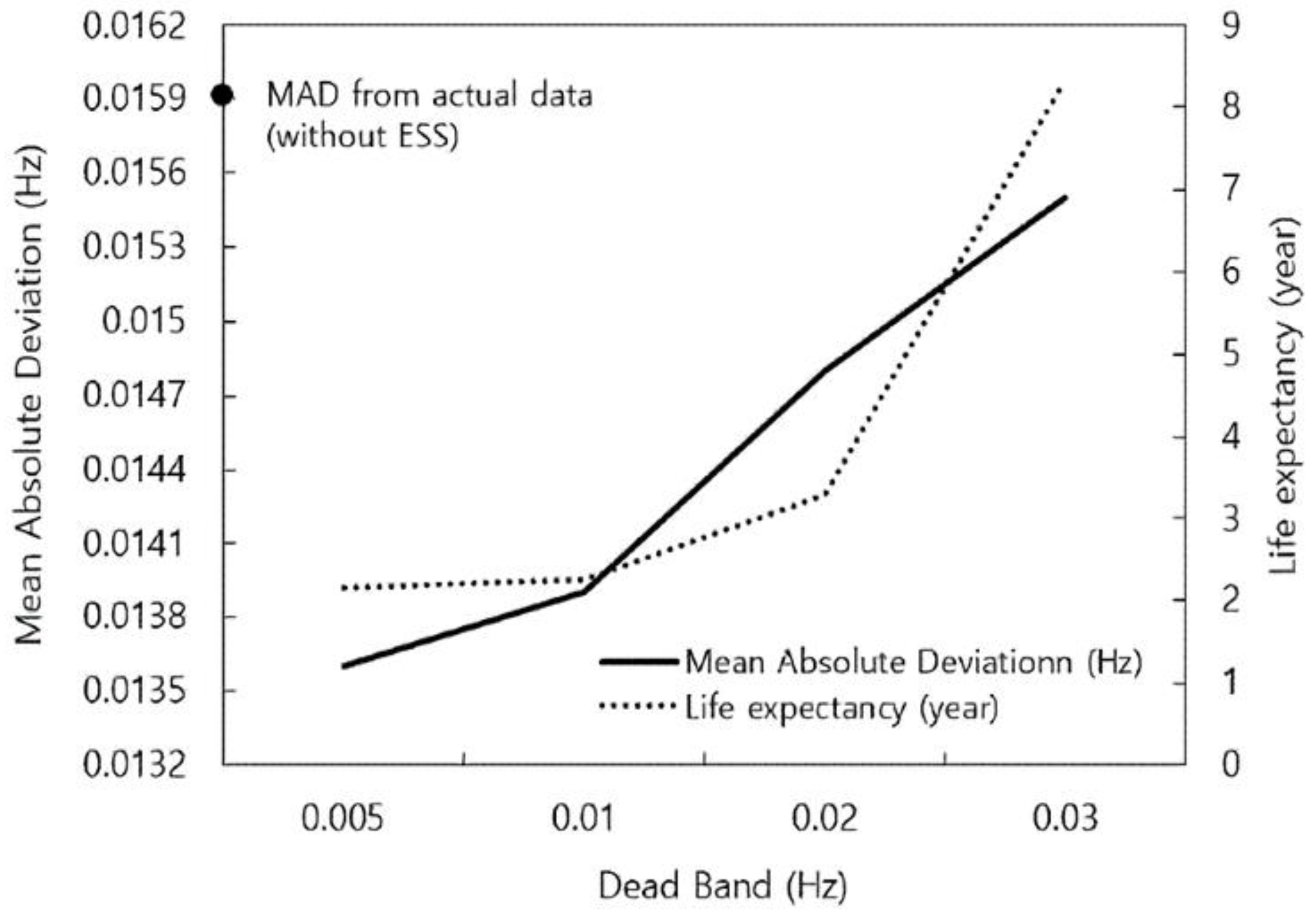
4.2. Dead-Band
4.3. SoC Recovery Range
5. Conclusions
Author Contributions
Funding
Data Availability Statement
Conflicts of Interest
Nomenclature
| µ | Charging and discharging efficiency |
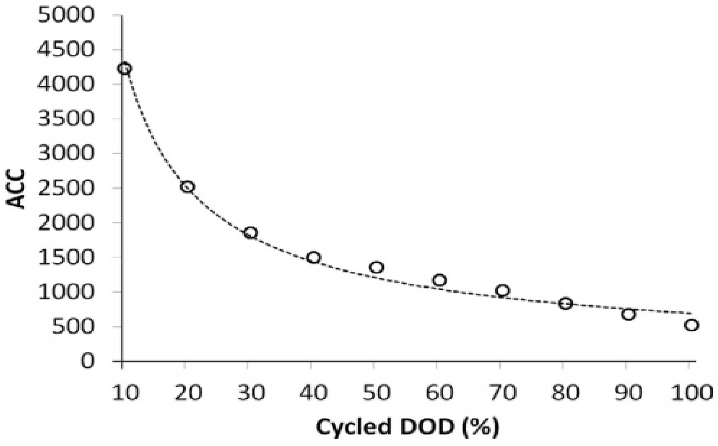
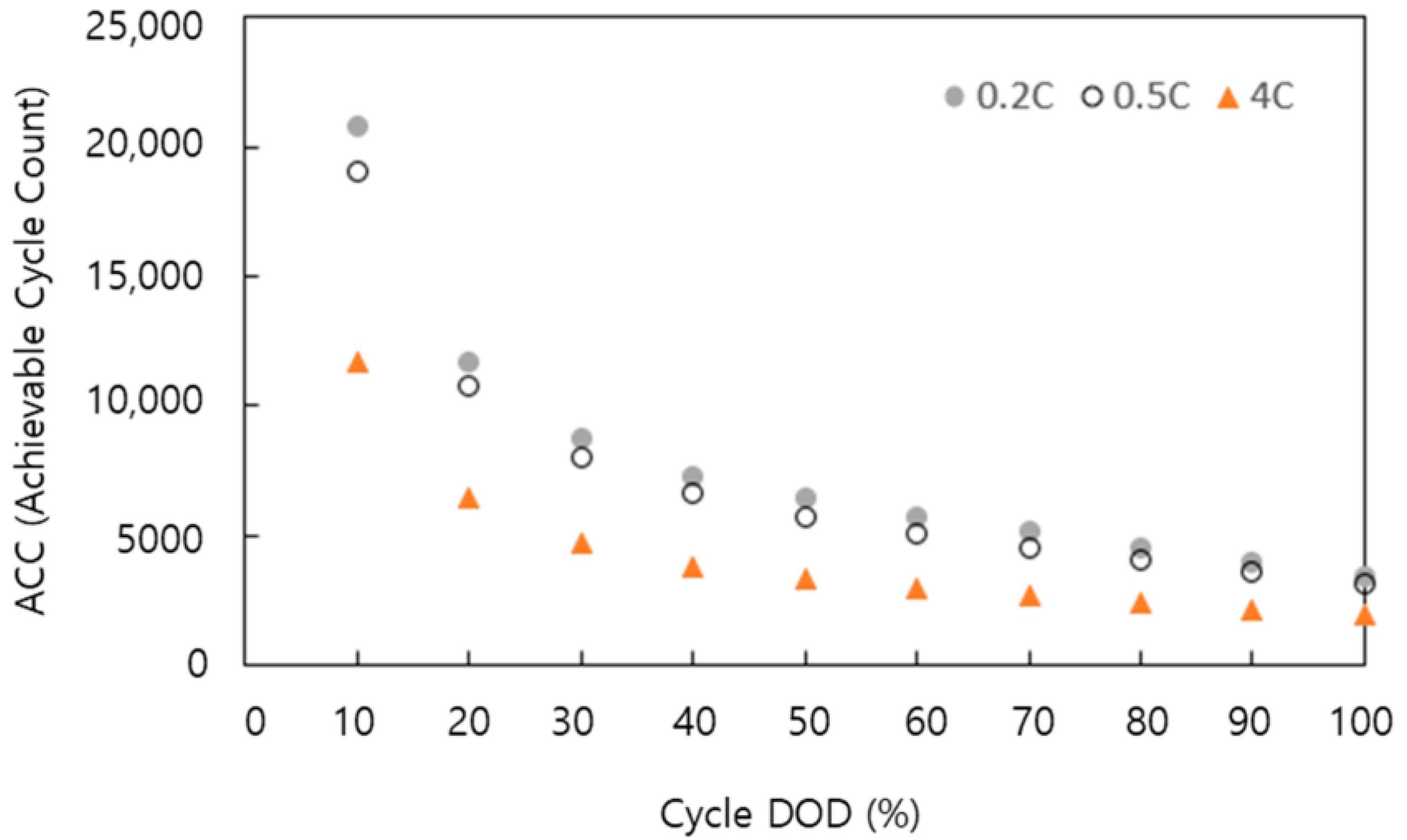
| ACC | Achievable cycle count |
| AWC | Average wear cost |
| BESS | energy storage system |
| C-rate | |
| CC | Constant current |
| C-rate | Rate of charge/discharge |
| CV | Constant voltage |
| DOD | depth of discharge |
| EoL | Specific end-of-life |
| ETS | Cycle energy during each transient state |
| Change in frequency | |
| Change measure frequency | |
| Change regulated frequency | |
| FR | Frequency regulation |
| I/O | input/output |
| K | Relationship between generation amount and the frequency variation |
| KEPCO | Korea Electric Power Corporation |
| MAD | mean absolute deviation |
| Number of annual transient states | |
| Change in BESS power | |
| Change in grid power | |
| Change in total power | |
| Amount of battery energy during | |
| Cycle energy for each time frame | |
| ΔS | SoC interval |
| S | Instance in the SoC interval |
| SoC | |
| SOC | State-of-charge |
| SoH | State of health |
| t | Time index during the given period |
| Change in time | |
| Duration of each transient state. | |
| Wd | AWC |
| WDF | Density function |
| WSS | Wear cost per MWh for the steady state |
| WTS | Wear cost per MWh for the transient state |
References
- Khalid, A.; Stevenson, A.; Sarwat, A.I. Overview of Technical Specifications for Grid-Connected Microgrid Battery Energy Storage Systems. IEEE Access 2021, 9, 163554–163593. [Google Scholar] [CrossRef]
- Amoasi Acquah, M.; Kodaira, D.; Han, S. Real-Time Demand Side Management Algorithm Using Stochastic Optimization. Energies 2018, 11, 1166. [Google Scholar] [CrossRef] [Green Version]
- KEPCO to Open Large-Capacity ESS Market for Power Frequency Regulation-ETNews. Available online: http://english.etnews.com/news/article.html?id=20140416200005 (accessed on 12 August 2020).
- Alt, J.T.; Anderson, M.D.; Jungst, R.G. Assessment of utility side cost savings from battery energy storage. IEEE Trans. Power Syst. 1997, 12, 1112–1120. [Google Scholar] [CrossRef] [Green Version]
- Yun, J.Y.; Yu, G.; Kook, K.S.; Rho, D.H.; Chang, B.H. SOC-based control strategy of battery energy storage system for power system frequency regulation. Trans. Korean Inst. Electr. Eng. 2014, 63, 622–628. [Google Scholar] [CrossRef] [Green Version]
- Serrao, L.; Chehab, Z.; Guezennec, Y.; Rizzoni, G. An aging model of Ni-MH batteries for hybrid electric vehicles. In Proceedings of the 2005 IEEE Vehicle Power and Propulsion Conference, Chicago, IL, USA, 7 September 2005; pp. 78–85. [Google Scholar]
- Vetter, J.; Novák, P.; Wagner, M.R.; Veit, C.; Möller, K.C.; Besenhard, J.O.; Winter, M.; Wohlfahrt-Mehrens, M.; Vogler, C.; Hammouche, A. Ageing mechanisms in lithium-ion batteries. J. Power Sources 2005, 147, 269–281. [Google Scholar] [CrossRef]
- Broussely, M.; Biensan, P.; Bonhomme, F.; Blanchard, P.; Herreyre, S.; Nechev, K.; Staniewicz, R.J. Main aging mechanisms in Li ion batteries. J. Power Sources 2005, 146, 90–96. [Google Scholar] [CrossRef]
- Gismero, A.; Schaltz, E.; Stroe, D.I. Recursive state of charge and state of health estimation method for lithium-ion batteries based on coulomb counting and open circuit voltage. Energies 2020, 13, 1181. [Google Scholar] [CrossRef] [Green Version]
- Belt, J.R. Battery Test Manual for Plug-In Hybrid Electric Vehicles; Idaho National Lab. (INL): Idaho Falls, ID, USA, 2010. [Google Scholar]
- Christophersen, J.P.; Ho, C.D.; Motloch, C.G.; Howell, D.; Hess, H.L. Effects of Reference Performance Testing during Aging Using Commercial Lithium-Ion Cells. J. Electrochem. Soc. 2006, 153, A1406. [Google Scholar] [CrossRef]
- Kim, J.; Chun, H.; Kim, M.; Yu, J.; Kim, K.; Kim, T.; Han, S. Data-Driven State of Health Estimation of Li-Ion Batteries with RPT-Reduced Experimental Data. IEEE Access 2019, 7, 106987–106997. [Google Scholar] [CrossRef]
- Coleman, M.; Lee, C.K.; Hurley, W.G. State of health determination: Two pulse load test for a VRLA battery. In Proceedings of the IEEE Annual Power Electronics Specialists Conference, Jeju, Korea, 18–22 June 2006. [Google Scholar]
- Zhang, J.; Zhang, X. A novel internal resistance curve based state of health method to estimate battery capacity fade and resistance rise. In Proceedings of the 2020 IEEE Transportation Electrification Conference & Expo (ITEC), Chicago, IL, USA, 23–26 June 2020; pp. 575–578. [Google Scholar]
- Huet, F. A review of impedance measurements for determination of the state-of-charge or state-of-health of secondary batteries. J. Power Sources 1998, 70, 59–69. [Google Scholar] [CrossRef]
- Ng, K.S.; Moo, C.S.; Chen, Y.P.; Hsieh, Y.C. Enhanced coulomb counting method for estimating state-of-charge and state-of-health of lithium-ion batteries. Appl. Energy 2009, 86, 1506–1511. [Google Scholar] [CrossRef]
- Bhangu, B.S.; Bentley, P.; Stone, D.A.; Bingham, C.M. Nonlinear observers for predicting state-of-charge and state-of-health of lead-acid batteries for hybrid-electric vehicles. IEEE Trans. Veh. Technol. 2005, 54, 783–794. [Google Scholar] [CrossRef] [Green Version]
- Lee, S.; Kim, J.; Lee, J.; Cho, B.H. State-of-charge and capacity estimation of lithium-ion battery using a new open-circuit voltage versus state-of-charge. J. Power Sources 2008, 185, 1367–1373. [Google Scholar] [CrossRef]
- Dai, H.; Wei, X.; Sun, Z. A new SOH prediction concept for the power lithium-ion battery used on HEVs. In Proceeding of the 5th IEEE Vehicle Power and Propulsion Conference, Dearborn, MI, USA, 7–10 September 2009; pp. 1649–1653. [Google Scholar]
- Kim, I.S. A technique for estimating the state of health of lithium batteries through a dual-sliding-mode observer. IEEE Trans. Power Electron. 2010, 25, 1013–1022. [Google Scholar]
- Plett, G.L. Sigma-point Kalman filtering for battery management systems of LiPB-based HEV battery packs. Part 2: Simultaneous state and parameter estimation. J. Power Sources 2006, 161, 1369–1384. [Google Scholar] [CrossRef]
- Prada, E.; Di Domenico, D.; Creff, Y.; Bernard, J.; Sauvant-Moynot, V.; Huet, F. Simplified Electrochemical and Thermal Model of LiFePO 4 -Graphite Li-Ion Batteries for Fast Charge Applications. J. Electrochem. Soc. 2012, 159, A1508–A1519. [Google Scholar] [CrossRef] [Green Version]
- Han, S.; Han, S.; Aki, H. A practical battery wear model for electric vehicle charging applications. Appl. Energy 2014, 113, 1100–1108. [Google Scholar] [CrossRef]
- Jo, H.; Choi, J.; Agyeman, K.A.; Han, S. Development of frequency control performance evaluation criteria of BESS for ancillary service: A case study of frequency regulation by KEPCO. In Proceeding of the 2017 IEEE Innovative Smart Grid Technologies-Asia, Auckland, New Zealand, 4–7 December 2017; pp. 1–5. [Google Scholar]
- Pinsky, N.; O’Neill, L. Southern California Edison Company—Advanced Technology 2131. In Tehachapi Wind Energy Storage Project Technology Performance Report #3; Southern California Edison: Rosemead, CA, USA, 2015; pp. 714–934. [Google Scholar] [CrossRef]
- Electimes. Available online: http://electimes.com/article.asp?aid=1493265868144076005 (accessed on 12 August 2020).


| Steady-State (0.2C) | Transient State (4C Discharge and 0.2C Recovering Charge) | Combined Cycle (Steady-State + Transient State) | Manufacture Specific 80% DoD Cycle (0.5C) | |
|---|---|---|---|---|
| Wear cost per MWh | $347/MWh | $981/MWh | $360/MWh | $447/MWh |
| Wear cost per Mode | $5787/(16.66 MWh/day) | $3384/ (3.45 MWh/event) | - | $4291.2/ (9.6 MWh/cycle) |
| Annual wear cost | $2,108,867 | $16,922 | $2,125,789 | - |
Publisher’s Note: MDPI stays neutral with regard to jurisdictional claims in published maps and institutional affiliations. |
© 2022 by the authors. Licensee MDPI, Basel, Switzerland. This article is an open access article distributed under the terms and conditions of the Creative Commons Attribution (CC BY) license (https://creativecommons.org/licenses/by/4.0/).
Share and Cite
Park, J.; Choi, J.; Jo, H.; Kodaira, D.; Han, S.; Acquah, M.A. Life Evaluation of Battery Energy System for Frequency Regulation Using Wear Density Function. Energies 2022, 15, 8071. https://doi.org/10.3390/en15218071
Park J, Choi J, Jo H, Kodaira D, Han S, Acquah MA. Life Evaluation of Battery Energy System for Frequency Regulation Using Wear Density Function. Energies. 2022; 15(21):8071. https://doi.org/10.3390/en15218071
Chicago/Turabian StylePark, Jingyeong, Jeonghyeon Choi, Hyeondeok Jo, Daisuke Kodaira, Sekyung Han, and Moses Amoasi Acquah. 2022. "Life Evaluation of Battery Energy System for Frequency Regulation Using Wear Density Function" Energies 15, no. 21: 8071. https://doi.org/10.3390/en15218071