Topology Optimization Design of Micro-Channel Heat Sink by Considering the Coupling of Fluid-Solid and Heat Transfer

Abstract

To investigate the effect of the target weight coefficient on the structure design of the micro-channel heat sink, an innovative method for the topology optimization design of micro-channel structures with different bifurcation angles is adopted. In this study, the improved interpolation function, density filtering, and hyperbolic tangent projection methods are adopted to obtain a clear topological structure of the micro-channel heat sink. The heat transfer of the micro-channel heat sink under different bifurcation angles is compared. At the same time, the influence of the two different objective functions, heat transfer, and flow energy consumption, is analyzed in the topology optimization of micro-channel heat sinks. The results show that when the bifurcation angle is 135°, both the heat transfer and the average outlet temperature of the micro-channel heat sink obtain the maximum value, and the heat transfer effect is the best. With the increase of the heat transfer weighting coefficient, the distribution of solid heat sources in the main channel increases, and the refinement of the branch channels also increases. On the other hand, although the heat transfer effect of the micro-channel heat sink is the best, the corresponding flow energy consumption is larger.

1. Introduction

With the development of electronic components towards chip miniaturization and integration, the heat transfer problem caused by the high heat flux density will be a great challenge. The quality of the heat exchange problem will significantly affect the average temperature of the electronic components when they are working. Excessive average temperatures will reduce the service life, thereby reducing their thermal stability. In addition, the improvement of heat transfer performance will significantly reduce the energy consumption of the heat sink. Especially in the micro-channel heat sink, Tuekerman [1] first proposed a micro-channel water-cooled silicon integrated heat sink, which can take away 790 W/cm² of heat when the temperature difference between the inlet and outlet is 71 K. The micro-channel heat sink of this high-performance cooling device, which is conducive to energy conservation, low carbon, and environmental protection has become an important research field in recent years due to its huge heat transfer potential [2,3,4,5].

The traditional straight channel, V-channel, S-channel, and other high heat flux micro-channel heat sinks cannot meet the heat transfer requirements of heat sinks in special environments due to its low heat transfer capacity and large flow resistance. In order to design a micro-channel structure with high heat transfer, Bejan et al. [6] proposed a configuration theory, and the designed fluid channel is a tree-like network. The micro-channel structure designed by Li [7] and Peng [8], based on the configuration theory, can improve the heat transfer capacity and reduce flow resistance. Qu [9] studied the micro-pin-fin heat sink and the straight channel micro-channel heat sink, and found that the micro-pin-fin heat sink has a lower thermal resistance and better heat dissipation effect, but also has a higher pressure loss. Chein [10] et al. replaced the fluid in the micro-channel heat sink with nanofluids, and it was found that the performances were greatly improved when nanofluids were used as the coolants. Rahbarshahlan et al. [11] enhanced heat transfer by replacing some surfaces in the micro-channel with hydrophobic surfaces, and research shows that this method can reduce the flow rate of hydrophobic surfaces, reduce pumping power, and thus increase heat transfer. In addition, Rostamzadeh et al. [12] used a new multi-dimensional artificial characteristic-based (MACB) scheme, which is applied to different and complex geometries with heat transfer and forced convection, such as a heat exchanger, vortex tube, etc. However, this kind of structure design, based on previous traditional methods, design experience, experimental results, and other newly proposed methods has great limitations due to its small degree of freedom in design. Among the existing optimization techniques, the topology optimization method proposed by Bendsøe and Kikuchi [13] can be regarded as one of the most promising optimization tools, due to its large design freedom. These new methods could potentially integrate the topology optimization method to calculate the heat transfer topology optimization of heat sink. Borvall and Petersson [14] applied the variable density method topology optimization to the steady Stokes flow at a low Reynolds number for the first time, and established the basic model of variable density method topology optimization for fluid flow, which opened the research of scholars on fluid topology optimization. In terms of the topology optimization of thermal fluids, the variable density method has been used for the structural design of forced convection [15,16,17,18] and natural convection problems [19,20]. Dede [21] used the commercial finite element analysis software COMSOL Multiphysics to optimize heat conduction and heat convection problems, and the objective function was expressed in terms of minimizing the average temperature and flow energy dissipation. Yoon [15] proposed a two-dimensional variable density method topology optimization to deal with the forced convection heat transfer problem, and the objective function was the minimum thermal compliance. Zhang et al. [22] designed the nanofluid-cooled heat sink based on topology optimization, and the research shows that reducing the diameter of nanoparticles and increasing the volume fraction of nanoparticles are conducive to improving the heat transfer performance of the heat sink. In most studies, topology optimization problems are solved with a single-objective function, such as minimizing the domain average temperature or minimizing thermal compliance [23,24].

Multi-objective optimization involves minimizing or maximizing multiple mathematical objective functions [25,26]. When comparing single-objective optimization with multi-objective optimization, it is more difficult to produce a unique optimal solution; however, compromises can be made in different objective functions to make the overall objective as optimal as possible. Dong et al. [18] studied the influence of non-Newtonian fluid on heat transfer performance by taking minimizing fluid energy dissipation and maximizing recoverable heat power as objective functions under the condition of a given solid heat source. Based on the variable density topology optimization method, Koga et al. [16] took the weighting function of heat transfer and flow energy dissipation as the objective function, and studied the influence of different weighting coefficients and inlet boundary conditions on the heat sink topology. Lv and Liu [27] used the topology optimization method to design the flow channel of the micro-channel heat sink for electronic components. In the optimization, the maximization of heat transfer and the minimization of pressure drop were taken as objective functions, and the effects of different penalty factors, fluid inlet flow rates, and weighting coefficients on the topology structure of the heat sink were investigated. Ghasemi et al. [28] dealt with the heat transfer problem of a pin-fin heat exchanger based on topology optimization method, and optimized the geometric water tank with minimizing the thermal resistance and pressure loss as the objective function. The optimization results show that the optimized topology exhibits superior cooling performance with reduced pressure loss.

Based on the structure topology optimization design method of variable density, the flow equation and the convective heat transfer equation are coupled, and the optimization model of the micro-channel heat sink with an indefinite solid heat source is established. Using a new interpolation function, the performance of micro-channel heat sinks with different bifurcation angles is studied by numerical simulation. Considering the two objective functions, maximizing heat transfer and minimizing flow energy consumption, the topology optimization design of the micro-channel heat sink is carried out by using different target weight coefficients.

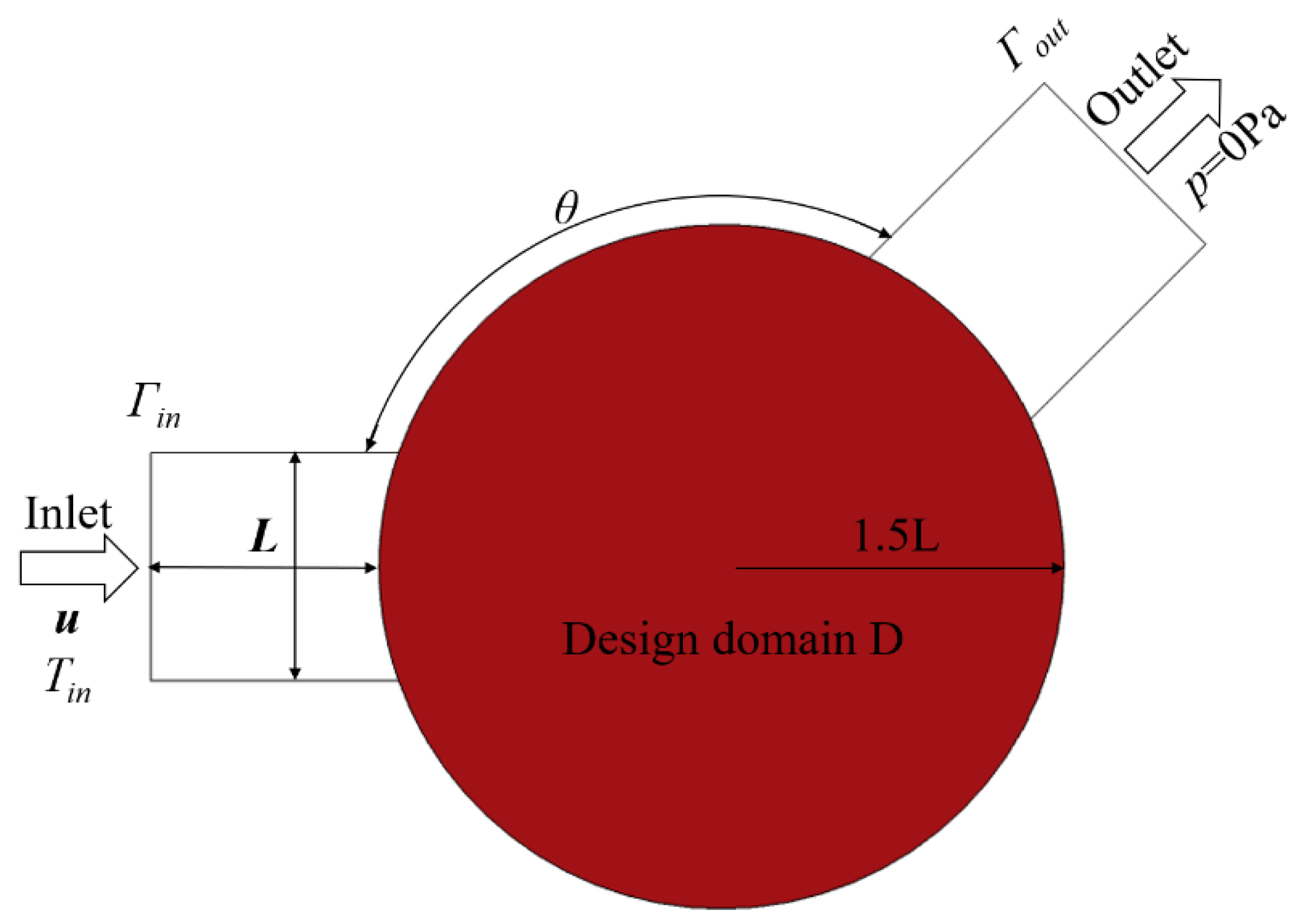
2. Physical Model

The design model of the fluid-structure coupled with the heat transfer of the micro-channel heat sink is shown in Figure 1. The red area D represents the design domain. The bifurcation angle between the inlet and outlet of the heat sink system is set to θ. The parameter L is the inlet and outlet width of the heat exchange system, which is set to 1mm, and the inlet temperature T_in is set to 273.15 K. In addition, the Reynolds number and Prandtl number at the inlet are 100 and 6.97 (the standard value of water), respectively. The fluid flow at the outlet directly flows into a large water tank without resistance, so the gauge pressure is set to 0 Pa. Γ_in and Γ_out represent the inlet and outlet boundaries of the design system, respectively, corresponding to the Dirichlet boundary and the Neumann boundary, and other boundaries are no-slip, adiabatic boundary conditions.

2.1. Governing Equations

In this study, the fluid flow problem is assumed to be the viscous incompressible steady flow, and the fluid flow model can be expressed as:

$$\rho \left(\mathit{u}\cdot \nabla \right)\mathit{u}+\nabla p-\mu \nabla \cdot \left[\nabla \mathit{u}+{\left(\nabla \mathit{u}\right)}^T\right]=\mathit{F}$$

(1)

$$\nabla \cdot \mathit{u}=0$$

(2)

where u, $\rho ,$ and p represent the flow velocity, density and pressure of the fluid, respectively, μ represents the dynamic viscosity of the fluid, and F represents the body force of the fluid flow.

The governing equation of the heat transfer field can be written as:

$$\rho c_p\left(\mathit{u}\cdot \nabla \right)T=k{\nabla }^{2}T+Q$$

(3)

where T denotes the temperature of the design domain, k denotes thermal conductivity, c_p denotes constant pressure heat capacity, and Q denotes the heat production per unit volume of the solid domain.

2.2. Topology Optimization Model Based on Variable Density Method

In the variable density topological optimization model of steady Navier-Stokes flow, the optimization problem is solved by adding a body force F, including the design variable $\gamma$, to the Navier-Stokes equations. Therefore, the body force in Equation (1) can be expressed as:

$$F=-\alpha \left({\gamma }_p\left(\gamma \right)\right)\mathit{u}=-\alpha \left(\gamma \right)\mathit{u}$$

(4)

where $\alpha \left(\gamma \right)$ is the resistance coefficient of artificial porous media, which is controlled by the design variable $\gamma$. In the variable density method, the design variable $\gamma$ represents the distribution of materials in the design domain, which varies continuously from 0 to 1, and $\gamma =0$, $\gamma =1$ correspond to the solid and fluid domains in the design domain, respectively. Since the design variables between 0 and 1 have no practical significance, the introduction of the interpolation function ${\gamma }_p$ eliminates more intermediate design variables (intermediate density), which in turn reduces the grayscale of the final optimization result. where the interpolation function ${\gamma }_p$ is defined as:

$${\gamma }_p\left(\gamma \right)=\frac{q\left(1-\gamma \right)}{q+\gamma }$$

(5)

where q is the penalty factor, and its influence on the interpolation function is shown in Figure 2a. The smaller the q value is, the greater the degree of aggregation of design variables to both ends of 0/1 by the interpolation function ${\gamma }_p$, which is conducive to avoiding the generation of intermediate density. And when $\gamma \in \left(0, 0.1\right)$ and q = 0.01, its influence on the interpolation function is most obvious, that is, it reduces the function value from 1 to 0 in the smallest $\gamma$ change. Therefore, in this optimization process, q value is 0.01.

However, the use of the above-mentioned interpolation function still inevitably leads to an undesired grayscale phenomenon in the final optimization result. Therefore, in this study, the generation of grayscale is further suppressed by further difference of the interpolation function ${\gamma }_p$. The interpolation function of ${\gamma }_p$ is expressed as:

$$\alpha \left({\gamma }_p\left(\gamma \right)\right)={\alpha }_{\min }+{\alpha }_{\max }\cdot f\left({\gamma }_p\right)$$

(6)

$$f\left({\gamma }_p\right)=a\cdot e^{-b\cdot {\gamma }_p}+c$$

(7)

where $f\left({\gamma }_p\right)$ is the interpolation function of the newly added ${\gamma }_p$. In traditional research, $f\left({\gamma }_p\right)={\gamma }_p$ is taken. The comparison is shown in Figure 2b. When ${\gamma }_p$ is close to the intermediate value, the newly added interpolation function $f\left({\gamma }_p\right)$ is significantly larger than the traditional method, which in turn increases the Darcy friction of the intermediate material and inhibits the appearance of the intermediate variable value. Therefore, this improved method can further reduce the gray level of the optimization domain, so as to achieve a better optimization effect. ${\alpha }_{max}$ and ${\alpha }_{min}$ are the minimum and maximum values of $\alpha$, respectively, and represent the resistance coefficient of the liquid and solid phases, respectively. The resistance coefficient of the liquid phase is very small, which is set to 0 in this paper. The value of the resistance coefficient of the solid phase ${\alpha }_{max}$ is determined by the Darcy number Da and the characteristic length L, which is written as:

$${\alpha }_{\max }=\frac{\mu }{Da\cdot L^2}$$

(8)

In topology optimization of the fluid-structure coupled heat transfer problem using the variable density method, we redefine material properties and heat source distribution to ensure the difference in material properties of the solid domain, the fluid domain, and a single heat source that generates heat only in solid domain. Based on this, the interpolation function relationship between material properties and design variables ${\gamma }_p$, and the heat source are defined as:

$$k\left({\gamma }_p\left(\gamma \right)\right)=k_f+\left(k_s-k_f\right)f\left({\gamma }_p\right)$$

(9)

$$c_p\left({\gamma }_p\left(\gamma \right)\right)=c_p{}_f+\left(c_p{}_s-c_p{}_f\right)f\left({\gamma }_p\right)$$

(10)

$$\rho \left({\gamma }_p\left(\gamma \right)\right)={\rho }_f+\left({\rho }_s-{\rho }_f\right)f\left({\gamma }_p\right)$$

(11)

$$Q\left({\gamma }_p\left(\gamma \right)\right)=\beta \left(1-f\left({\gamma }_p\right)\right)\left(T_{\mathrm{ref}}-T\right)$$

(12)

$$\beta =a\cdot k_f/L^2$$

(13)

where k is the thermal conductivity; c_p is the heat capacity at constant pressure. The subscripts f and s represent fluid materials and solid materials, respectively. In addition, the thermophysical parameters of the fluid and solid materials are shown in

Table 1. Physical properties of materials.

Material	k (W/m/K)	cp (J/kg/K)	$\mathit{\rho }$
Fluid	0.6	4180	1000
Solid	238	900	2700

. Β is the heat generation coefficient which controls the speed of the heat generation [5] and a is a constant, and the value is 167. T_ref is the reference temperature, which is 298 K. Combining Equations (5), (7), and (12), it can be seen that when the design variable $\gamma =1$ (representing the fluid domain), the amount of heat production per unit volume Q is 0, that is, no heat is produced in the fluid flow region.

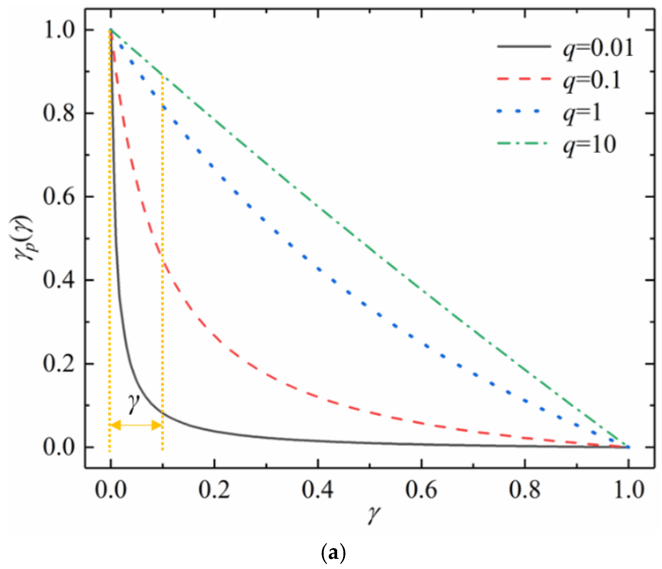
2.3. Filter and Projection

In the optimization process, in order to ensure the smoothness of the design variable distribution, it needs to be filtered by the Partial Differential Equation (PDE) filter. PDE filter. The design variables are filtered using the Helmholtz partial differential equation [29,30], which is defined as:

$$-R^2{\nabla }^2{\gamma }_f+{\gamma }_f={\gamma }_c$$

(14)

where R is the filter radius, which is selected as the minimum grid size in this paper; ${\gamma }_c$ is the design variable before filtering; and ${\gamma }_f$ is the design variable after filtering.

Helmholtz partial differential equation filtering design variables can solve problems such as grid dependence and smoothness of the distribution of design variables. However, it also increases the overall grayscale of the design domain, resulting in a large amount of gray area (intermediate density) between the solid and fluid materials in the design domain. In order to reduce the grayscale of the design area, the hyperbolic tangent projection method is used in the filtered design area, which is expressed as:

$$\gamma =\frac{\tanh \left({\beta }_{\gamma }\left({\gamma }_f-{\gamma }_{\beta }\right)\right)+\tanh \left({\beta }_{\gamma }{\gamma }_{\beta }\right)}{\tanh \left({\beta }_{\gamma }\left(1-{\gamma }_{\beta }\right)\right)+\tanh \left({\beta }_{\gamma }{\gamma }_{\beta }\right)}$$

(15)

where $\gamma$ is the design variable after projection; ${\gamma }_{\beta }$ is the projection point, and its value is 0.5. ${\beta }_{\gamma }$ is the projection slope, and its influence on the projection is shown in Figure 2c. The larger the value of ${\beta }_{\gamma }$, the steeper the curve is, and the better the polarization distribution effect of design variables; however, it will also lead to instability of the calculated value and poor convergence. In order to improve the stability and convergence of the optimization problem, and avoid the optimization problem from falling into a local optimal solution, we adopt the continuous approach, that is, take a small value of ${\beta }_{\gamma }$ in the initial stage of the optimization iteration, gradually increase the value of ${\beta }_{\gamma }$, and finally make the fluid-solid boundary gradually clear [31].

3. Multi-Objective Optimization

The optimization of the fluid-structure interaction heat transfer needs to consider the problem of fluid target, thermal target, and solid distribution, at the same time. The problem of solid distribution is solved by adding a body force containing the design variable $\gamma$ to the Navier-Stokes equations. For the fluid target and thermal target, weigh the importance of the two and adjust the proportion of the two targets to meet the actual engineering needs. Therefore, it is necessary to establish a multi-objective optimization equation first, then calculate a set of Pareto optimal solutions, and finally select the optimal solution according to the actual needs.

The larger the heat transfer in the design domain, the better the heat transfer effect. In addition, the smaller the flow energy consumption, the smaller the flow loss. Therefore, the first optimization objective considered in this study is to maximize the heat exchange in the entire design area, and the second optimization objective is to minimize the flow energy dissipation in the whole design area. The heat exchange and flow energy consumption are defined as:

$$J_1={\displaystyle {\int }_{\Omega }\beta \left(1-\gamma \right)\left(T_{\mathrm{ref}}-T\right)}d\Omega$$

(16)

$$J_2={\displaystyle {\int }_{\Omega }\left[\mu \left(\nabla \mathit{u}+\nabla {\mathit{u}}^{\mathrm{T}}\right):\left(\nabla \mathit{u}+\nabla {\mathit{u}}^{\mathrm{T}}\right)+\alpha {\mathit{u}}^2\right]}d\Omega$$

(17)

In the study, the simple additive weighting (SAW), that is, the linear weighted summation method, is used to combine the above two optimization objectives. In order to avoid an invalid weighting coefficient, due to the difference of the calculation results of the two functions, J₁ and J₂ need to be normalized. The normalization processing method is used to perform scaling processing on the above single-objective function, and the scaling processing method is as follows:

$$J_i{}^{\prime }=\frac{J_i^{max}-J_i\left(\gamma \right)}{J_i^{max}-J_i^{min}}$$

(18)

where I takes the value of 1 and 2. $J_i^{max}$ and $J_i^{min}$ represent the maximum and minimum values of the objective function, respectively.

Therefore, the multi-objective function weighted by the objective functions of heat exchange J₁ and flow energy consumption J₂ are expressed as follows:

$$J\left(\mathit{u},T,\gamma \right)={\omega }_1{J}_1{}^{\prime }-{\omega }_2{J}_2{}^{\prime }$$

(19)

where J is the multi-objective function, ω₁ and ω₂ are the weighting coefficients of heat exchange and flow energy consumption, respectively. The expression of the multi-objective function can be controlled by adjusting the size of the weighting coefficient, and then different optimization structures can be obtained. However, if the values of ω₁ and ω₂ are not constrained, many repeated cases will be obtained, which is meaningless and is not conducive to the subsequent analysis of the results. For example, the working condition of ω₁ = 0.1, ω₂ = 0.2 and the working condition of ω₁ = 1, ω₂ = 2 are repeated. Therefore, we set $0\le {\omega }_1\le 1$,$0\le {\omega }_2\le 1$, and ${\omega }_1=1-{\omega }_2$, and when ${\omega }_1>0.5$, the design domain takes the maximum heat exchange as the main objective function, that is, the objective function of heat exchange dominates, otherwise the design domain takes the minimum flow energy dissipation as the main objective function.

Based on the above model analysis, the mathematical expression of the multi-objective topology optimization of the fluid-structure coupled heat transfer system is as follows:

$$\begin{array}{l}max:J\left(\mathit{u},T,\gamma \right)\\ \mathrm{s}.\mathrm{t}.\left\{\begin{array}{l}\rho \left(\mathit{u}\cdot \nabla \right)\mathit{u}+\nabla p-\mu \nabla \cdot \left[\nabla \mathit{u}+{\left(\nabla \mathit{u}\right)}^T\right]=-\alpha \mathit{u}\\ -\nabla \cdot \mathit{u}=0\\ \rho c_p\left(\gamma \right)\left(\mathit{u}\cdot \nabla \right)T=k\left(\gamma \right){\nabla }^{2}T+Q\left(\gamma \right)\\ 0\le \gamma \le 1\end{array}\right.\end{array}$$

(20)

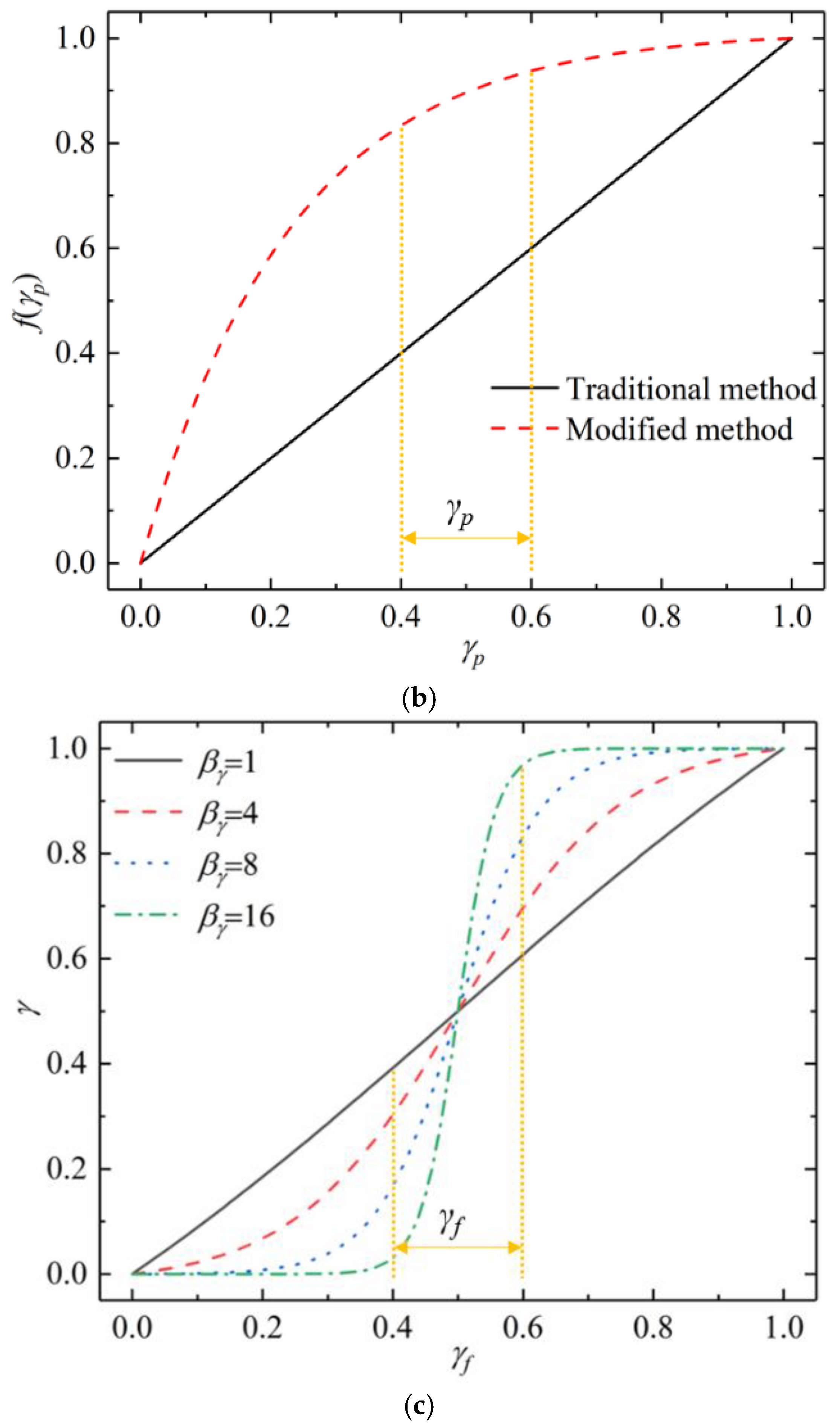
4. The Solution Process of Topology Optimization

The calculation and optimization problems are identified by the interface between the commercial finite element software COMSOL Multiphysics 5.6 [32] and MATLAB [33]. The computational fluid dynamics module (CFD) and fluid heat transfer module (ht) are used to compute related problems such as fluid flow and heat transfer, respectively. The design domain is discretized using bilinear finite elements [34]. Free triangular meshes are used to generate meshes by controlling the maximum mesh size, and the dependence of calculation results on meshes is eliminated through projection and filtering. The convergence criterion of the optimization process is defined as:

$$\left|\left(J_n-J_{n-1}\right)/J_n\right|\le \epsilon$$

(21)

where, n is the number of calculation iteration steps, $\epsilon =1\times {10}^{-8}$. If the calculation results of the two iteration steps in the optimization process conform to Equation (21), or the maximum number of iteration steps is reached, then the iteration is terminated.

The flow chart of the solution process for the topology optimization of the micro-channel heat sink is shown in Figure 3. The optimization process includes the following main steps:

(1)

Give the initial value of the design variable $\gamma$ in the design domain.

(2)

Solve equations at various current parameters.

(3)

Calculate the objective function and constraints.

(4)

Calculate the design sensitivity under the current concomitant variables.

(5)

Update the design variable $\gamma$ using the Global Convergence Method of Moving Asymptotes (GCMMA).

(6)

Loop the above (2)–(5) steps until the iteration termination condition is met.

5. Results and Discussions

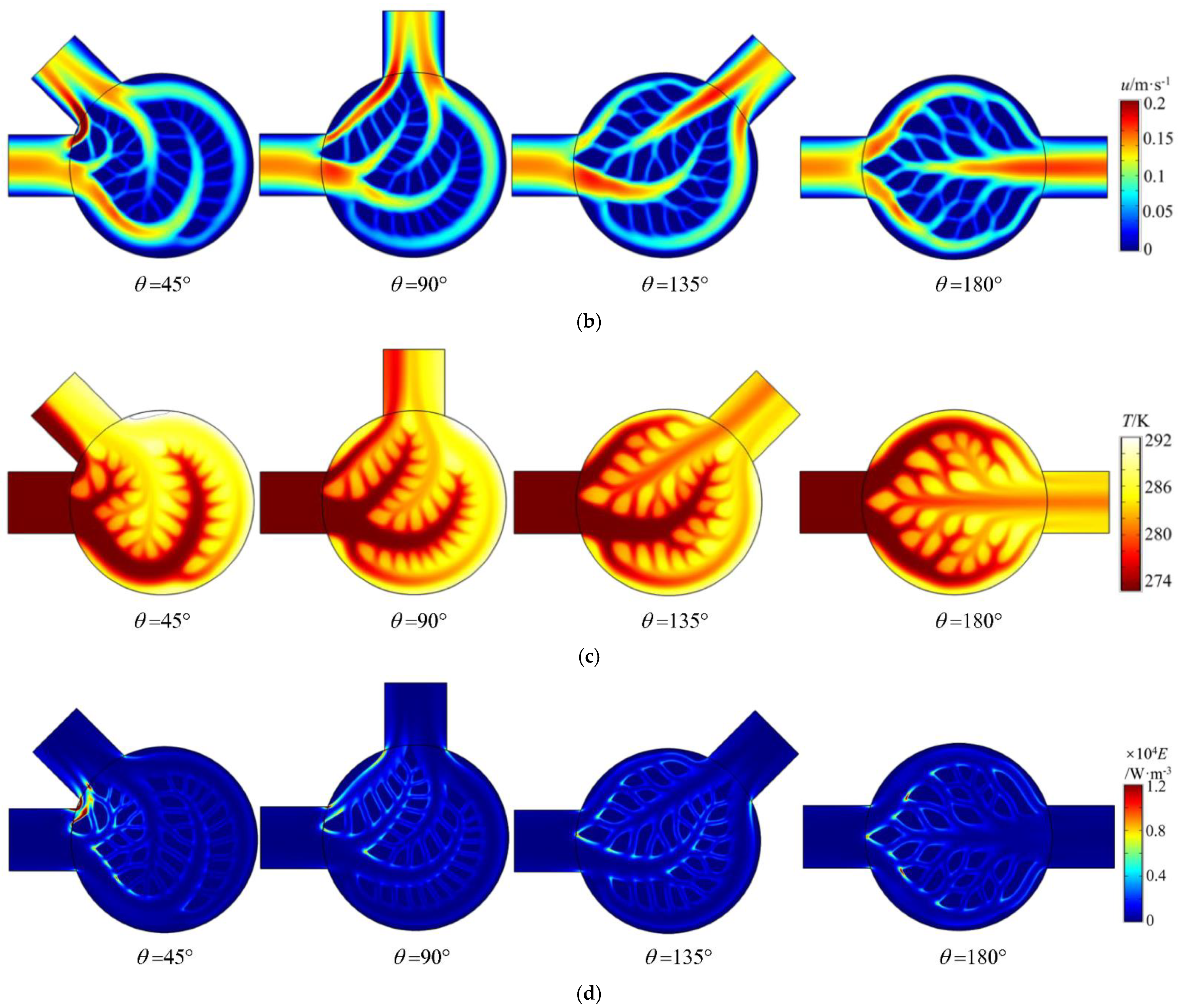
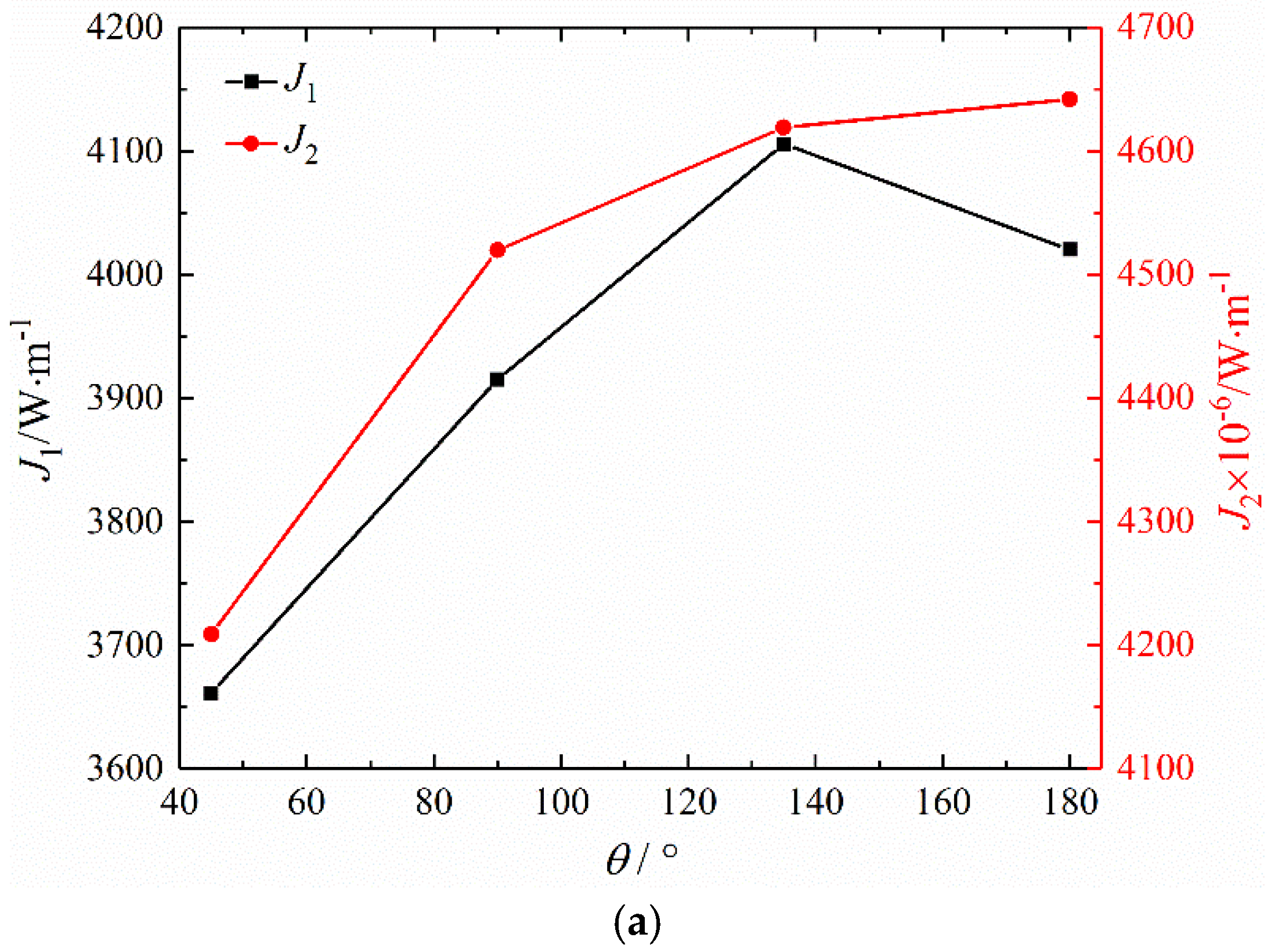
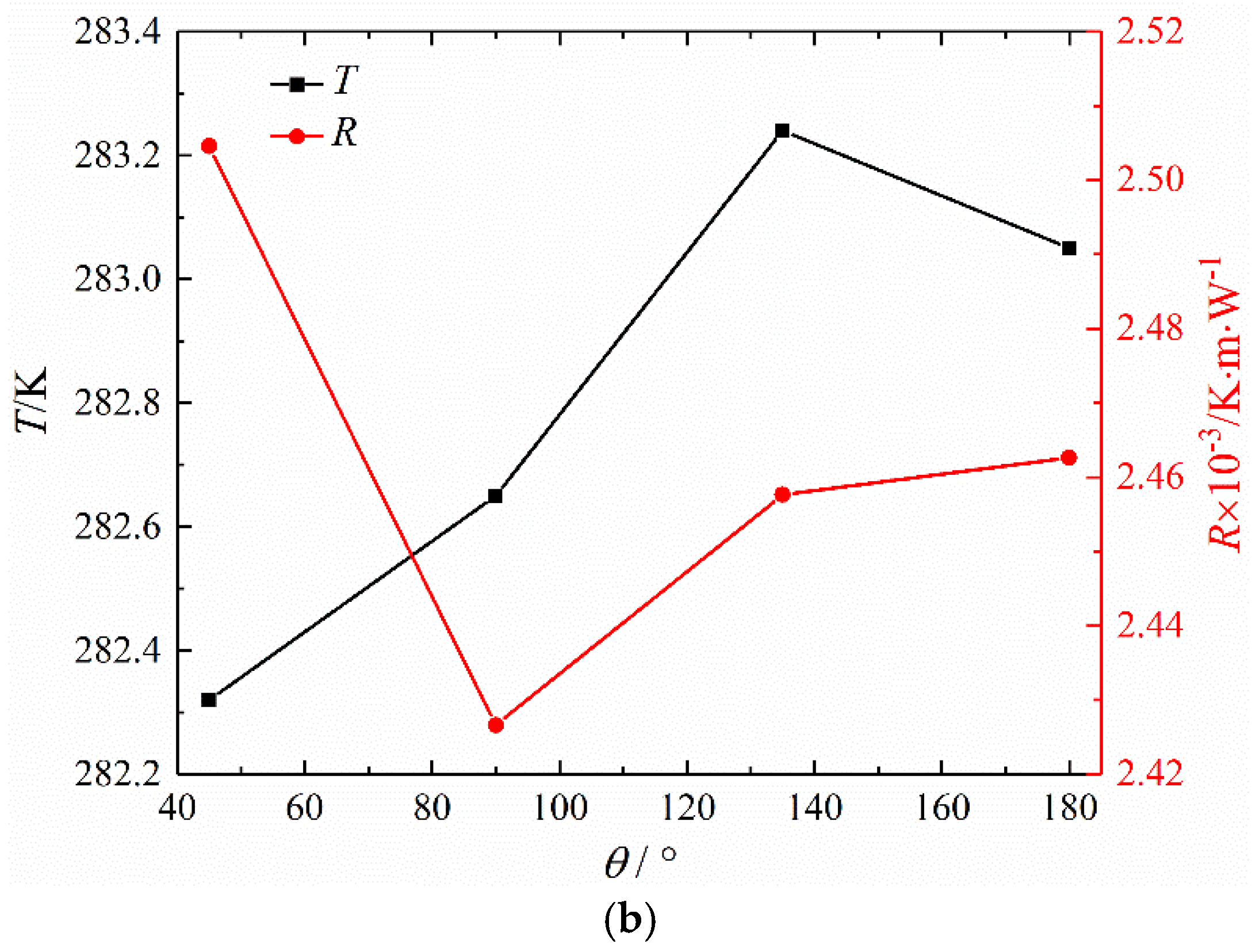
5.1. Micro-Channel Heat Sink Optimization under Different θ

In practical engineering applications, different inlet and outlet angle distributions can be selected. Therefore, it is necessary to study the influence of different inlet and outlet positions on the heat transfer, flow energy consumption, and average outlet temperature in the design domain. Taking $J_1^{\prime }$ as the objective function, that is, selecting ω₁ = 1 and ω₂ = 0 in Equation (18), the topology structure with the best heat transfer performance under different bifurcation angles θ is studied.

The optimal topological structure and its velocity field, temperature field, and energy dissipation density field distribution under different bifurcation angles are shown in Figure 4. In the optimal topology, the white and black regions represent the fluid and solid regions, respectively, and their corresponding design variables are 1 and 0, respectively. However, the design variables in the grey area are between 0 and 1, which represent intermediate material densities, which have no practical significance and should be eliminated as much as possible in the optimal topology. It can be seen from Figure 4 that the density of the intermediate material in this study has been well eliminated, indicating that the interpolation function $f\left({\gamma }_p\right)$ used in this paper has played a good role.

Comparing the optimal topological structures under four different bifurcation angles, it can be found that the flow channel structures have certain similarities: The fluid flow channel has two to three main channels distributed from the inlet to the outlet. The fluid flows into the heat sink from the inlet, and is divided by the solid heat source in the design domain when it flows through it, and finally converges in the outlet channel and flows out after the heat exchange in the design domain. The solid heat sources in the optimized design domain show a scale-like distribution, which is different from the conventional heat sink, and these scale-like distributions of solid heat sources lead to the refinement of many tiny flow channels in the heat sink. However, the difference is that with the change of the bifurcation angle, the position of the solid heat source, that acts as a diverter at the entrance of the design domain, also changes and the smaller the bifurcation angle is, the closer it is to the edge of the entrance. Correspondingly, the position of the solid heat source at the outlet of the design domain, which plays the role of collecting fluid, also changes similarly. This leads to a large curvature of the fluid flowing through the inlet and outlet channels of the heat sink under a small bifurcation angle, and its flow distance is small, which is not conducive to fluid flow and heat exchange.

Comparing the velocity field and temperature field at different bifurcation angles, it is obvious that the velocity distribution and temperature distribution are similar to the above-mentioned flow channel structure. For the heat sink with θ = 45°, a part of the flow channel connecting the inlet and outlet is short and narrow, and the overall flow channel is tapered. As a result, when the fluid flows through this part of the fine flow channel, the degree of bending changes greatly, the flow velocity increases sharply, and the velocity gradient is large, which in turn leads to high fluid flow velocity, insufficient heat exchange, and uneven outlet temperature. In addition, it can be found from Figure 4 that for the heat sink with large bifurcation angles, the inlet and outlet channels are distributed farther, the flow channels in the design domain are fully extended, the distance of fluid flow is longer, the fluid heat exchange is more sufficient, and the outlet temperature is more uniform. It is these fully extended scaly-like distributions of solid heat sources and tiny flow channels that make the outlet velocity and temperature distribution of the heat sink under large bifurcation angles more uniform, and the average temperature of the entire design domain lower, which also shows that the heat transfer performance of a micro-channel heat sink with the large bifurcation angle is better.

The energy dissipation density distribution under different bifurcation angles is shown in Figure 4d. By comparison, it can be found that the areas with high energy dissipation density are all distributed in the solid heat source side impacted by the fluid, which is also the area with large flow loss in the microchannel heat sink. On the side of a solid heat source that is not impacted by fluid, the energy dissipation density is small, and the corresponding flow loss is small. In particular, when the bifurcation angle of the microchannel heat sink is 45° and 90°, the fluid curvature flowing through the inlet and outlet channels of the heat sink is large, and the energy dissipation density is also greatly increased, which can be clearly shown in Figure 4d. However, the energy dissipation density distribution of the microchannel heat sink with bifurcation angles of 135° and 180° is relatively uniform.

Figure 5 shows the variation of the heat exchange J₁, the flow energy consumption J₂, the average outlet temperature T, and the thermal resistance R, with the bifurcation angle θ in the design domain. The thermal resistance R is defined as follows:

$$R=\frac{T-T_{in}}{J_1}$$

(22)

where T denotes the average outlet temperature, T_in denotes the inlet temperature, which is set at 273.15 K, and J₁ denotes the heat exchange of the design domain.

With the increase of the bifurcation angle θ, the J₁, J₂, and T of the optimized domains all show an increasing trend, and R tends to decrease first and then increase. In particular, when θ = 135°, the heat exchange J₁ and the average outlet temperature T reach their peaks. The flow energy consumption J₂ does not increase, and the thermal resistance R is relatively small when θ > 135°. Compared with the small bifurcation angle, the increase of J₁ and T are larger, and the increase of energy dissipation J₂ is relatively small, and compared with the large bifurcation angle, J₁ and T are larger, and J₂ is smaller. In particular, although the heat resistance R of the micro-channel heat sink at θ = 90° is the smallest, the heat exchange and the average outlet temperature at this time are smaller. In addition, compared with the optimal topology of the heat sink with θ = 135° and θ = 180° in Figure 4, it can be seen that when the fluid flows through the heat sink with θ = 135°, more fluid flows through the upper and middle flow channels, and after heat exchange with the solid heat sources on both sides of the flow channel, it gathers in other flow channels and flows out. Correspondingly, when the fluid flows through the heat sink with θ = 180°, the fluid is divided into the upper and lower main branch channels and flows out after heat exchange with the solid heat source at the side of the central channel. However, the scale-like distribution of solid heat sources of the heat sink with θ = 135° is more compact than that of the heat sink with θ = 180°, and the heat transfer between fluid and heat source is more sufficient. As shown in Figure 5, the average temperature at the outlet is higher, and the heat transfer in the design domain is greater. Therefore, in this study, the bifurcation angle of 135° with better comprehensive performance will be selected for subsequent multi-objective optimization.

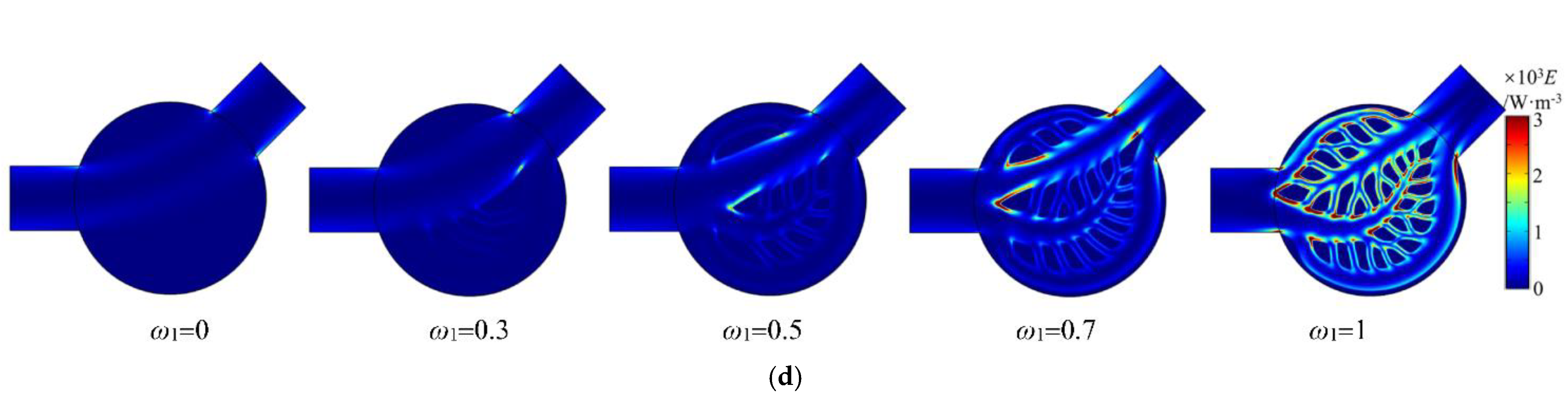
5.2. Micro-Channel Heat Sink Optimization under Different ω₁

In order to study the performance characteristics under different weighting coefficients ω₁, micro-channel heat sinks under different ω₁ were selected for analysis. Figure 6 shows the optimal topology, velocity field, temperature field and energy dissipation density field distribution under different ω₁. Comparing the optimal topological structures under different ω₁, it can be found that when ω₁ = 0, the flow channel of the micro-channel is the main channel connecting the inlet and outlet, and no branches appear. After the fluid flows into the design domain from the inlet, it flows directly through the main channel and flows out from the outlet. This is because the objective function J₁ of heat exchange under this working condition does not contribute to the multi-objective function J, and the optimization objective degenerates into a single-objective function that minimizes the flow energy dissipation J₂. With the increase of ω₁, the proportions of J₁ and J₂ in the multi-objective function J increase and decrease, respectively, which means that the objective function of heat exchange gradually dominates. At this time, the main channel connecting the inlet and outlet of the micro-channel is gradually shunted by the solid heat source, and the area of the main channel is reduced. The branch channels appear preferentially below the main channel, and gradually expand to the entire optimization domain, and the branch channels are gradually further refined by the scaly-like distribution of solid heat sources. In particular, when ω₁ = 1, the flow energy dissipation J₂ does not contribute to the multi-objective function J, and the optimization objective degenerates into a single-objective function that minimizes heat exchange J₁. The fluid at the entrance of the optimization domain is completely diverted by the solid heat source, and the main channel no longer exists, but is refined into several tributaries by a large number of scaly-like distribution of solid heat sources. Compared with the working condition of ω₁ < 1, the distribution of the solid heat source is more refined, and the small tributaries are more diverse. We comprehensively analyzed the optimal topology and energy dissipation density, and found that the area with a large energy dissipation density was also distributed on the solid heat source side impacted by the fluid. The smaller the weighting coefficients ω₁ is, the smaller the energy dissipation density of the whole heat sink domain is. This change trend also matches the flow energy dissipation in the optimization goal.

In addition to the above optimal topological structures under different ω₁, we also compared and analyzed the corresponding velocity field and temperature field, which was similar to the above flow channel distribution. As there is no branching effect, the flow is the smoothest, and the flow energy dissipation is also the smallest; the contact between the fluid and the solid wall is only the wall part of the main channel, so the fluid-solid contact area is the smallest and the heat transfer effect is the worst, which corresponds to the objective function after degeneration. With the increase of ω₁, in addition to flowing through the main channel, the fluid flow in the design domain will also be divided by the branch flow channels. The larger the ω₁, the smaller the area occupied by the main channel, the more scaly-like distribution of solid heat sources, the more branch flow channels, and the more obvious the diversion effect. The above features also mean that the fluid-solid contact area is increased, thus the fluid flow energy dissipation is increased, and the corresponding heat transfer effect is also improved. When ω₁ = 1, the fluid-solid contact area reaches the maximum value, and the fluid flow becomes the most complicated. The fluid flows out from the three branch flow channels and several small channels, and the energy dissipation increases greatly. At the same time, the fluid takes away the heat of the optimization domain to the greatest extent, and the heat transfer effect is greatly increased. We can also find from Figure 6 that when ω₁ is large, the temperature distribution of the entire design domain is more even, with no large temperature gradient, which is more reasonable.

Figure 7 shows the optimal solutions, Pareto frontier, and optimal configuration under different weighting factors, where the single-objective functions J₁ and J₂ are the abscissa and ordinate, respectively. The Pareto frontier of the micro-channel heat sinks in this paper all have the characteristics of an upward convex curve, which is consistent with the convex function shape described by Timothy et al. [35]. Its topological structure change has obvious regularity with the increase of ω₁: the branch channels are preferentially split under the main runner, and the main channel is slowly replaced by the upper, middle and lower branch channels. The distribution of the solid heat source tends to be uniform and presents a scaly-like distribution, the aspect ratio of a single solid heat source gradually decreases, and the shape of the solid heat source evolves from a large strip to a small square (approximately). Using the linear logarithmic transform function (Log3P1) to perform nonlinear curve fitting on the Pareto frontier, the fitting equation is obtained using Equation (23). Based on this equation, engineering designers can select the corresponding performance parameters according to their actual engineering needs, and the optimal design has been achieved.

$$J_1=9466.9+1005.5\times \log \left(J_2-4.377\times {10}^{-5}\right)$$

(23)

Figure 8 shows the heat exchange J₁, flow energy dissipation J₂, the average outlet temperature T and the thermal resistance R under different weighting coefficients ω₁. According to the comparative analysis of Figure 7, it can be concluded that for the optimal topology with ω₁ < 0.3, the fluid directly flows through the main channel connecting the inlet and outlet of the design domain, with no branches and small channels, so J₁, J₂, T, and R do not change much. For the optimal topology with ω₁ = 0.3, there are branch flow channels in the lower part of the main channel; however, most of the fluid still flows out through the main channel, and J₁ and J₂ show little change. Compared to the working condition of ω₁ = 0.2, J₁ increases by 670 W/m, J₂ increases by 0.11 Mw/m, T increases by 3 K, and R decreases by 0.58 × 10⁻³ K∙m/W. For the optimal topology with ω₁ > 0.3, the branch flow channels near the main runner are gradually refined and increased, so J₁, J₂, and T also gradually increase, and correspondingly, R gradually decreases. In particular, for the optimal topology with ω₁ = 0.8, the fluid at the inlet is completely shunted by the solid heat source, and the main flow channel is reduced to no longer exist. Therefore, the increase of J₁ is larger than that of ω₁ < 0.8, and the J₂ is also greatly increased. When ω₁ = 0.8, the average outlet temperature reaches the maximum value, the flow energy consumption is smaller than that of ω₁ > 0.8, and the change of heat transfer is not large. Therefore, when choosing the best topology design, we can pay special attention to the case where the main channel is reduced until it no longer exists.

5.3. Mesh Independence Test

We take ω₁ = 1 and θ = 135° as an example to verify the mesh independence. The optimal structure under three different mesh sizes is shown in the Figure 9, and the mesh size selected in this paper is the medium mesh. The mesh number, heat exchange J₁, flow energy consumption J₂, average outlet temperature T, and its relative former difference of the micro-channel heat sink are shown in

Table 2. Mesh details for the mesh independence test.

Mesh Number	J1/W∙m−1	Relative Former Difference (J1)	J2/W∙m−1 (×10−6)	Relative Former Difference (J2)	T/K	Relative Former Difference (T)
(a) 68,250	4033.1	×	4614.6	×	283.07	×
(b) 97,386	4105.6	1.80%	4619.1	0.10%	283.24	0.06%
(c) 131,815	4149.1	1.06%	4608.9	−0.22%	283.35	0.04%

. In addition, the cell dimensions of the coarse mesh, medium mesh, and fine mesh are L/50, L/60, and L/70, respectively. The mesh independence test shows that the optimal topology under different mesh sizes is consistent on the whole, while there are some differences in the distribution of scale-like solid heat sources in some regions. The relative former difference of parameters under different mesh sizes is very small, which also shows that the final optimization design result is independent of the number of meshes. Therefore, the medium mesh size selected in this paper is reasonable and reliable.

6. Conclusions

The method of topology optimization design is used to study the micro-channel heat sink by considering the coupling of fluid-solid and heat transfer. Based on the two objective functions of achieving high heat transfer capacity and low flow energy dissipation, a multi-objective function is proposed to optimize the structure topology of the heat sink, and the influences of the inlet and outlet bifurcation angles and heat transfer weighting coefficients on the optimal topology of the radiator are revealed. The main conclusions are as follows.

• In the numerical implementation of topology optimization design, the improved interpolation function, PDE filter, and hyperbolic tangent projection effectively eliminate the gray area of the topology structure and tiny solid particles, which improve the smoothness of the flow channels and avoid checkerboard results.
• The optimal topology of the micro-channel heat sink has obvious regularity with the change of θ. With the increase of θ, the overall performance parameters show a monotonically increasing trend. Among them, the heat exchange and the average outlet temperature reach the maximum value when θ = 135°, and the overall flow energy dissipation is relatively small. Therefore, in the selection of the heat sink, different bifurcation angles can be considered based on the calculation results, rather than the intuitive or empirical selection of θ = 180°.
• Based on the multi-objective topology optimization design, micro-channel heat sinks with different heat transfer weighting coefficients are obtained. When minimizing energy dissipation dominates, the heat sink is occupied by the main channel connecting the inlet and outlet, and the fluid mainly flows out through the main flow channel with few branch flow channels. Its flow energy dissipation is smaller and the heat exchange effect is worse. When the maximum heat exchange is dominant, the main channel of the heat sink is filled with scaly-like distribution of solid heat sources, and the main channel gradually shrinks and is replaced by the upper, middle, and lower branch channels. In addition, the branch flow channels are further refined into many tiny flow channels, which makes the heat exchange effect of the heat sink better and the flow energy consumption larger.

References

- Tuckerman, D.B.; Pease, R.F.W. High-performance heat sinking for VLSI. IEEE Electron Device Lett. 1981, 2, 126–129. [Google Scholar] [CrossRef]
- Qu, W.L.; Mudawar, I. Experimental and numerical study of pressure drop and heat transfer in a single-phase micro-channel heat sink. Int. J. Heat Mass Transf. 2002, 45, 2549–2565. [Google Scholar] [CrossRef]
- Afzal, H.; Kwang-Yong, K. Shape optimization of micro-channel heat sink for micro-electronic cooling. IEEE Trans. Compon. Packag. Technol. 2008, 31, 322–330. [Google Scholar] [CrossRef]
- Alperen, Y.; Sertac, C. Multi objective optimization of a micro-channel heat sink through genetic algorithm. Int. J. Heat Mass Transf. 2020, 146, 118847. [Google Scholar] [CrossRef]
- Zhang, B.; Zhu, J.G.; Gao, L.M. Topology optimization design of nanofluid-cooled microchannel heat sink with temperature-dependent fluid properties. Appl. Therm. Eng. 2020, 176, 115354. [Google Scholar] [CrossRef]
- Bejan, A.; Errera, M.R. Convective trees of fluid channels for volumetric cooling. Int. J. Heat Mass Transf. 2000, 43, 3105–3118. [Google Scholar] [CrossRef]
- Li, Y.L.; Zhang, F.L.; Sunden, B.; Xie, G. Laminar thermal performance of microchannel heat sinks with constructal vertical Y-shaped bifurcation plates. Appl. Therm. Eng. 2014, 73, 183–193. [Google Scholar] [CrossRef]
- Peng, Y.; Liu, W.Y.; Chen, W.; Wang, N. A conceptual structure for heat transfer imitating the transporting principle of plant leaf. Int. J. Heat Mass Transf. 2014, 71, 79–90. [Google Scholar] [CrossRef]
- Qu, W.L. Comparison of thermal-hydraulic performance of singe-phase micro-pin-fin and micro-channel heat sinks. In Proceedings of the 11th Intersociety Conference on Thermal and Thermomechanical Phenomena in Electronic Systems, Orlando, FL, USA, 28–31 May 2008. [Google Scholar] [CrossRef]
- Chein, R.; Huang, G. Analysis of microchannel heat sink performance using nanofluids. Appl. Therm. Eng. 2005, 25, 3104–3114. [Google Scholar] [CrossRef]
- Rahbarshahlan, S.; Esmaeilzadeh, E.; Khosroshahi, A.R.; Bakhshayesh, A.G. Numerical simulation of fluid flow and heat transfer in microchannels with patterns of hydrophobic/hydrophilic walls. Eur. Phys. J. Plus 2020, 135, 157. [Google Scholar] [CrossRef]
- Rostamzadeh, A.; Razavi, S.E.; Mirsajedi, S.M. Towards Multidimensional Artificially Characteristic-Based Scheme for Incompressible Thermo-Fluid Problems. Mechanika 2017, 23, 826–834. [Google Scholar] [CrossRef] [Green Version]
- Bendsøe, M.P.; Kikuchi, N. Generating optimal topologies in structural design using a homogenization method. Comput. Methods Appl. Mech. Eng. 1988, 71, 197–224. [Google Scholar] [CrossRef]
- Borrvall, T.; Petersson, J. Topology optimization of fluids in Stokes flow. Int. J. Numer. Methods Fluids 2003, 41, 77–107. [Google Scholar] [CrossRef]
- Yoon, G.H. Topological design of heat dissipating structure with forced convective heat transfer. J. Mech. Sci. Technol. 2010, 24, 1225–1233. [Google Scholar] [CrossRef]
- Koga, A.A.; Lopes, E.C.C.; Villa Nova, H.F.; de Lima, C.R.; Silva, E.C.N. Development of heat sink device by using topology optimization. Int. J. Heat Mass Transf. 2013, 64, 759–772. [Google Scholar] [CrossRef]
- Yaji, K.; Yamada, T.; Yoshino, M.; Matsumoto, T.; Izui, K.; Nishiwaki, S. Topology optimization in thermal-fluid flow using the lattice Boltzmann method. J. Comput. Phys. 2016, 307, 355–377. [Google Scholar] [CrossRef]
- Dong, X.; Liu, X.M. Multi-objective optimal design of microchannel cooling heat sink using topology optimization method. Numer. Heat Transf. A Appl. 2020, 77, 90–104. [Google Scholar] [CrossRef]
- Alexandersen, J.; Aage, N.; Andreasen, C.S.; Sigmund, O. Topology optimisation for natural convection problems. Int. J. Numer. Methods Fluids 2014, 76, 699–721. [Google Scholar] [CrossRef] [Green Version]
- Alexandersen, J.; Sigmund, O.; Aage, N. Large scale three-dimensional topology optimisation of heat sinks cooled by natural convection. Int. J. Heat Mass Transf. 2016, 100, 876–891. [Google Scholar] [CrossRef]
- Dede, E.M. Multiphysics topology optimization of heat transfer and fluid flow systems. In Proceedings of the COMSOL Users Conference, Boston, MA, USA, 30 March 2009; Available online: https://www.comsol.com/paper/download/44388/Dede.pdf (accessed on 5 June 2021).
- Zhang, B.; Zhu, J.H.; Xiang, G.X.; Gao, L. Design of nanofluid-cooled heat sink using topology optimization. Chin. J. Aeronaut. 2021, 34, 301–317. [Google Scholar] [CrossRef]
- Yaji, K.; Yamada, T.; Kubo, S.; Izui, K.; Nishiwaki, S. A topology optimization method for a coupled thermal-fluid problem using level set boundary expressions. Int. J. Heat Mass Transf. 2015, 81, 878–888. [Google Scholar] [CrossRef]
- Łaniewski-Wołłk, Ł.; Rokicki, J. Adjoint Lattice Boltzmann for topology optimization on multi-GPU architecture. Comput. Math. Appl. 2016, 71, 833–848. [Google Scholar] [CrossRef]
- Sato, Y.; Yaji, L.; Izui, K.; Yamada, T.; Nishiwaki, S. An optimum design method for a thermal-fluid device incorporating multiobjective topology optimization with an adaptive weighting scheme. J. Mech. Des. 2018, 140, 31402. [Google Scholar] [CrossRef]
- Guirguis, D.; Hamza, K.; Aly, M.; Hegazi, H.; Saitou, K. Multi-objective topology optimization of multi-component continuum structures via a Kriging-interpolated level set approach. Struct. Multidiscip. Optim. 2015, 51, 733–748. [Google Scholar] [CrossRef]
- Lv, Y.; Liu, S. Topology optimization and heat dissipation performance analysis of a micro-channel heat sink. Meccanica 2018, 53, 3693–3708. [Google Scholar] [CrossRef]
- Ghasemi, A.; Elham, A. Multi-objective topology optimization of pin-fin heat exchangers using spectral and finite-element methods. Struct. Multidiscip. Optim. 2021, 64, 2075–2095. [Google Scholar] [CrossRef]
- Lazarov, B.S.; Sigmund, O. Filters in topology optimization based on Helmholtz-type differential equations. Int. J. Numer. Methods Eng. 2011, 86, 765–781. [Google Scholar] [CrossRef]
- Kawamoto, A.; Matsumori, T.; Yamasaki, S.; Nomura, T.; Kondoh, T.; Nishiwaki, S. Heaviside projection based topology optimization by a PDE-filtered scalar function. Struct. Multidiscip. Optim. 2011, 44, 19–24. [Google Scholar] [CrossRef]
- Li, H.; Ding, X.H.; Meng, F.Z.; Jing, D.; Xiong, M. Optimal design and thermal modelling for liquid-cooled heat sink based on multi-objective topology optimization: An experimental and numerical study. Int. J. Heat Mass Transf. 2019, 144, 118638. [Google Scholar] [CrossRef]
- Available online: https://www.comsol.com/ (accessed on 5 June 2021).
- Available online: https://www.mathworks.com/ (accessed on 5 June 2021).
- Tezduyar, T.E.; Mittal, S.; Ray, S.E.; Shih, R. Incompressible flow computations with stabilized bilinear and linear equal-order-interpolation velocity-pressure elements. Comput. Methods Appl. Mech. Eng. 1992, 95, 221–242. [Google Scholar] [CrossRef]
- Timothy, W.A.; Panos, Y.P. A note on weighted criteria methods for compromise solutions in multi-objective optimization. Eng. Optim. 1996, 27, 155–176. [Google Scholar] [CrossRef]