Pythagorean Fuzzy Storage Capacity with Controllable Carbon Emission Incorporating Green Technology Investment on a Two-Depository System

Abstract

Global warming is mainly caused by carbon emissions. Currently, fewer countries are concentrating on reducing carbon emissions. The primary strategy utilized by numerous countries to achieve carbon emissions reduction is the carbon tax policy. With this in mind, a sustainable two-warehouse inventory model was taken carbon tax into account for a controllable carbon emissions rate by investing in green technology initiatives under uncertain emission and cost parameters. The globe is currently experiencing an eco-friendly period. Many individuals are interested in purchasing natural or herbal items since they are made from natural sources and do not affect the environment. The demand for products made with herbal or natural ingredients is considered eco-friendly demand. This study examines a two-warehouse inventory model of deteriorating commodities with price and marketing-dependent eco-friendly demand. The inventory system is presented to handle the inventory in the depository with last-in-first-out and first-in-first-out strategies. After comparing both the policies under deterioration rate and holding cost, this study recommended a suitable dispatch policy. Interval-valued numbers and fuzzy numbers are the mathematical techniques that deal with uncertainties, so this model’s emission and cost parameters are taken as interval-valued numbers, and the storage capacity of the owned warehouse is a Pythagorean fuzzy number. The optimal solution for the two-warehouse inventory system is evaluated by taking the parametric form of interval-valued cost parameters and the new concept of the ranking function of triangular Pythagorean fuzzy numbers. Numerical results prove that emissions are reduced by 87% under green technology investment in both policies. As a consequence, in the FIFO policy, the total cost of the two-warehouse inventory system decreases by 34.45% and cycle length increases by 5.72%, and in the LIFO policy, the total cost of the two-warehouse inventory system decreases by 34.42% and cycle length increases by 11.19%. Sensitivity analysis of the key parameters has been performed to study the effect of various parameters on the optimal solution.

1. Introduction

The warehouse’s job is to keep products safe and secure. Typically, two-warehousing concepts are utilized to keep inventory: owned warehouse (OW) and rental warehouse (RW). In general, RW has more amenities than OW, and also have to pay rent; therefore, the holding cost in RW will be higher, and the degradation rate will be lower owing to the additional facilities. Holding costs are the extra expenses for maintaining and storing inventory in the warehouse. Holding costs play a key role in the two-warehouse inventory management system. If the holding cost of the commodities is high, then the total cost of the inventory system also increases. Therefore, researchers should focus on reducing holding costs while considering two-warehouse problems. Due to competition in depository marketing, the holding cost of RW is sometimes less than or equal to the holding cost of OW; thus, this study examines all such scenarios and recommends an appropriate dispatch strategy.

To reduce inventory costs, this model considers last-in-first-out (LIFO) and first-in-first-out (FIFO) techniques. This study will utilize the LIFO policy to sell the items that arrive last at the depository, and will store the goods that arrive later in RW because retailer will sell the last incoming goods first, lowering the warehouse rent; otherwise, the retailer will have to pay a large inventory rent. To reduce degradation, retailer will sell the first incoming material using FIFO. OW deteriorates faster than RW; if retailer keeps first in and first out material in OW first, he may sell it first, lowering the deterioration rate and allowing retailers to sell more fresh items to clients. The FIFO method is best for badly degraded products, whereas the LIFO method is better for minimizing high holding costs of RW. Ishii and Nose [1] proposed a two-warehouse inventory system with selling prices depending on warehouse capacity. Dye et al. [2] developed an inventory system based on OW’s restricted capacity because of varying item degradation rates in the two warehouses. Das et al. [3] proposed a two-warehouse-based supply chain presuming that the market warehouse’s holding cost is higher than the RW’s. Liang and Zhou [4] presented a two-warehouse-based inventory system on the premise that the degradation of OW is more significant than RW, but the holding cost of OW is less than RW. Bhunia et al. [5] established a two-warehouse system assuming that the deterioration rate in RW is lower than the deterioration rate in OW for various holding costs. This model considered all the variations of holding costs and deterioration rates of OW and RW based on actual market conditions.

In warehouse management, the deterioration of items is a common problem and de pends upon a time, varying with the item. If the deterioration rate is high, such item spoils in less time those items call semi-durable products, such as milk, vegetable, fish, etc. If the deterioration rate is less, then the item does not spoil in less time; those items are called durable products, such as plastic toys, motor parts, electrical equipment, etc. A warehouse inventory model has been presented under different deterioration rates ([6,7,8,9]). No matter how much time passes, the item’s technical characteristics are maintained owing to the preservation technique. Consequently, by investing in preservation technologies, we may slow down the rate at which goods deteriorate. Tsao [10] proposed a supply chain system of deteriorating items under preservation technology. Giri et al. [11] developed an inventory model by assuming time-dependent degradation and investing in preservation techniques.

Demand plays a major role in inventory management; without considering the demand, retailers cannot estimate the inventory for future use. These days most customers prefer to buy eco-friendly products since eco-friendly products are made with herbal or natural ingredients, do not present any side effects, etc. The usage of natural or herbal ingredients in the product impacts the demand for that item, concluding that the order depends on the usage of herbal or natural ingredients. Researchers consider various types of demands in their inventory models. Rong et al. [12] presented a warehouse inventory system of selling price-dependent demand rate under fuzzy lead time. Lee and Hsu [13] created an inventory model by considering the demand rate’s stock dependence under preservation technology. Bhavani et al. [14] proposed an inventory model by assuming the demand rate as a function of reliability and time.

In real-life scenarios, most things are imprecise due to uncertainty. Many of the inventory models are developed under uncertain environments. Kannan et al. [15] developed a green supply chain under an intuitionistic fuzzy environment. Mahapatra et al. [16] developed an inventory model under an uncertain environment by assuming cost parameters as triangular fuzzy numbers. Wu et al. [17] presented an inventory system with a demand that depends on the stock incorporating the deterioration of items.

Transportation costs play an important role in an inventory system. The relationship between transport and the environment is conflicting regarding environmental issues. Transport is responsible for a significant quantity of hazardous emissions, which in turn leads to problems that are both detrimental to society and the environment and expensive to fix. However, this portion of transportation emissions rises yearly, and consequently, the freight movement’s impact on the eco-system has altered the ecological system and done tremendous damage. Because of all these effects, this study has considered transportation emission costs, holding emission costs and deteriorating emission costs of OW and RW and developed this model in a sustainable environment. In recent days, researchers develop their models under sustainability. Das et al. [18] developed a multi-objective transportation problem by considering emission costs under a fuzzy environment. Taleizadeh [19] et al. and Murmu et al. [20] developed their inventory models under the emission policy. Energy consumption of transportation cost depends on fuel price ([21]). This model’s transportation cost depends on fuel price, distance, fuel consumption, and the number of shipments.

Green investment helps control carbon emissions by reducing the emission fraction to keep the environment clean and safe. Since consumers are increasingly interested in purchasing eco-friendly items, businesses are now interested in using green technologies to save inventory costs and boost brand value. Green warehousing is an advanced technique to implement business in a green environment through multiple ways to study depository inventory systems. By implementing a few changes, we may easily make the depository more eco-friendly without much difficulty; such simpler ways to make the warehouse green are: (i) upgrading warehouse high-efficiency lighting, (ii) investing in energy-efficient equipment, (iii) using fewer packing cuts down on waste, (iv) reuse and recycle materials, (v) build a green or cool roofing system, (vi) add solar panels to a depository, (vi) reduce waste as shown in Figure 1.

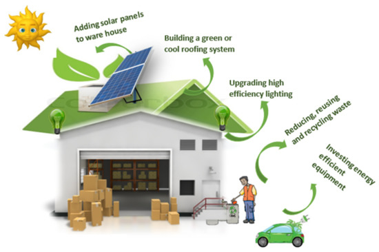
Figure 1. Characteristics of green warehouse.

This article is organized as follows. A review of the literature is provided in Section 1 and a discussion of the motivation for the study and the research gaps. The formulation of the FIFO and LIFO models along with the necessary preliminary information, notation (Appendix A), and presumptions, are included in Section 2. Section 3 contains the analysis of the FIFO and LIFO models with a carbon-tax policy under green technology. Section 4 provides a solution methodology for the total cost of the two-warehouse system under FIFO and LIFO policies. A case study with numerical example is provided in Section 5. Section 6 presents a sensitivity analysis of the key parameters of the two-warehouse inventory system and discusses some important managerial applications of the observations. Conclusions and future research directions are presented in Section 7.

1.1. Literature Review

1.1.1. Inventory Models under a Two-Warehouse Environment

Several papers have been published based on the notion of two-warehouse inventory models, assuming that the deterioration rate of RW is lower than the degradation rate of OW under various holding costs charges ([22,23,24]) and dispatching rules ([25]). Ouyang et al. [26] created an inventory system based on the assumption that OW’s capacity is smaller than the order amount. Howard et al. [27] developed a supply chain structure by considering numerous local warehouses. Gong and Wei [28] designed an updated adaptive genetic algorithm to optimize warehouse item inventory. Budiawan et al. [29] presented a drug application in inventory management employing the FIFO dispatch principle. Shu et al. [30] devised a challenge for optimizing depository placement using a location-inventory network design issue. Diabat and Theodorou [31] created a two-tier supply chain system with several warehouses dependent on location. This study contemplates a system to store highly deteriorated products to get the maximum benefit out of the concept.

1.1.2. Inventory Models under Preservation Technology

Preservation of a commodity is an essential issue in the inventory management system. It prevents the products from degrading while they are stored in the warehouse or store. In order to lessen the effects of deterioration, preservation technology is crucial. In this context, different business enterprises and organizations must use preservation technology in inventory control systems. The deterioration of commodities is a natural occurrence that cannot be prevented; however, when products are at risk of deterioration and obsolescence, they can be slowed down by specialized equipment or methods. For instance, food that has been packaged and stored is not stable indefinitely and eventually degrades to an unacceptably low level. Chemical deterioration and microbial spoilage are prevented by low temperatures, for instance, those found in refrigerators. Film and color materials last longer in cold storage. Therefore, the amount of money invested in the facility’s inventory preservation technology, as well as the environment there, determines how much of an item’s quality is degrading. This article emphasizes the significance of considering preservation technology investment. Preservation technology ([32]) prevents spoilage, damages items in the inventory, minimizes an item’s deterioration rate, and maximizes the deterioration time. Yang et al. [33] established a model by assuming a rate of deterioration is time-dependent and can be decreased by investing in preservation technology. A supply chain under preservation was developed by Yadav et al. [34], and the investment outcomes reveal that preservation technology reduced waste and improved the sustainability of the inventory system. Sepehri et al. [35] and Mishra et al. [36] proposed a model by investing separately in carbon emission reduction and preservation technology under a constant deterioration rate of items. This paper considered that both OW and RW deterioration rates are constant and follow the preservation technology in a two-warehouse inventory system. This model invested separately in carbon emission reduction and preservation technology. Investments in preservation technology can control the model’s decaying progress, and investments in green technology results can control the model’s carbon emissions and positively impact environmental sustainability.

1.1.3. Inventory Models under Various Demands

Several researchers work on a two-warehouse inventory system ([37,38]) by considering linear trend demand. Lee and Dye [39] developed an inventory model by assuming stock-dependent demand under preservation technology. Jaggi et al. [40] established a two-warehouse inventory scheme of constant demand under various dispatch policies by considering the holding cost of OW less than RW. Shastri et al. [41] proposed a supply chain inventory model of selling price-dependent demand. Smaila et al. [42] developed an inventory model by considering the quadratic demand rate. Jaggi et al. [43] developed various dispatch policies from a two-warehouse inventory system of constant demand. Dye et al. [44] established a supply chain under price-dependent demand with spending for preservation. Shaikh et al. [45] presented an inventory system with two-warehouse by considering interval-valued inventory parameters under stock-dependent demand. Xu et al. [46] designed a two-warehouse inventory model by assuming the demand rate as trapezoidal type demand. Sarkar et al. [47] proposed a production inventory system by taking price-dependent demand for the products. By considering the above discussion, this paper presumes the demand as price, the impact of advertisement and the proportion of chemical or herbal substances in the product.

1.1.4. Study under Various Uncertain Environments

Fuzzy numbers and interval-valued numbers are two sorts of mathematical tools for handling uncertainty. The generalizations of fuzzy and intuitionistic fuzzy sets are Pythagorean fuzzy sets (PFSs). Many two-warehouse-based inventory systems with varying demand have developed exciting literature ([48,49,50,51]) by researchers under fuzzy environments. Recently, some studies ([52,53]) included Pythagorean fuzzy uncertainty to develop their models. This study of the inventory system considers the capacity of OW as a triangular Pythagorean fuzzy number (TPFN).

1.1.5. Research under Green Warehouse, Carbon Tax, and Green Technology

Green warehousing is an advanced concept to reduce emissions in warehouse inventory systems. Paul et al. [54] developed a green inventory model by assuming that demand is influenced by the level of green concern and price. Technology that is environmentally friendly and developed and used in a way that does not harm the environment and conserves natural resources is known as green technology. It is also called sustainable technology or clean technology. Emissions may reduce with the use of green technology. Green technology is a system that uses innovative methods to create eco-friendly products. It uses renewable natural resources that never deplete, so the future generation can also benefit from it. It can effectively change waste patterns and production in a way that will not harm the planet. Pan et al. [55] and Sarkar et al. [56] considered green technology to reduce carbon emission and emission cost under carbon tax and carbon cap and trade policies. Daryanto et al. [57] developed a two-warehouse inventory model considering carbon emission. Li and Hai [58] developed an inventory system by considering carbon emissions. Cheng et al. [59] proposed a supply chain to invest in emission reduction investment under carbon trading and subsidy policies. Shen et al. [60] proposed a green supply chain model under sustainable and fuzzy uncertain environments. The proposed green warehouse model is developed under green technology by assuming that the amount of carbon emission released from both OW and RW reduces due to green technology and emission cost considered under carbon tax policy.

1.2. Motivation and Research Questions

After analyzing a few studies, it becomes clear that no research has been done so far that takes into account the triangular Pythagorean fuzzy imprecision, carbon emission, and investment in green technology in two-green-warehouse inventory models under FIFO and LIFO dispatching strategies. These encourage us to create a more particle-based two-warehouse inventory model that considers sustainability and preservation efforts. This research proposed a novel ranking system to convert triangular Pythagorean fuzzy numbers (TPFNs) into crisp numbers. As a result, imprecision does not exist, preservation prevents deterioration, and green technology lowers emissions in the problem-solving process.

In earlier work, the development of preservation and green expenses investing in emission and degradation reduction has not been offered together in a two-warehouse inventory system under FIFO and LIFO dispatching policies. The question of how a sustainable two-warehouse concept with both preservation and green investment can be implemented naturally arises. This work is accomplished with the use of sustainable models. Preservation and green technology with impreciseness of cost and emission parameters have not been used in two-warehouse models under dispatching policies only slightly implemented in their models. With this in mind, the two-warehouse model’s idea of green and preservation investments is used to reduce emissions and degradation, enhancing the realistic nature of the model. Two-warehouse inventory models under FIFO and LIFO policies influence demand, cost, and selling price. Table 1 shows the research gap. The research results provide a detailed understanding of the state of global carbon emission research.

Table 1. Contribution of this work compared to previous analogous studies.

FIFO and LIFO Policies	Price Reliant Demand	Advertisement Dependent Demand	% of Herbal and Chemical Ingredients Reliant Demand	Preservation Investment	Green Investment	Carbon Emission	Imprecise Parameter	Nature of Uncertainty	Reference
C	C	NC	NC	NC	NC	NC	NC	NC	Jaggi et al. [61]
NC	NC	NC	NC	NC	NC	C	NC	NC	Cheng et al. [62]
C	NC	NC	NC	NC	NC	NC	NC	NC	Xu et al. [63]
NC	C	C	NC	NC	NC	NC	Cost parameter	Triangular fuzzy	Mahapatra et al. [16]
NC	NC	NC	NC	NC	C	C	NC	NC	Huang et al. [64]
NC	C	NC	NC	C	C	C	NC	NC	Mishra et al. [36]
NC	C	C	NC	NC	NC	NC	NC	NC	Sanjose et al. [65]
C	C	NC	NC	NC	NC	NC	NC	NC	Rana et al. [66]
NC	NC	C	NC	NC	NC	NC	NC	NC	Barun et al. [67]
NC	NC	NC	NC	NC	C	C	NC	NC	Hasan et al. [68]
NC	C	NC	NC	NC	NC	C	Emission& cost parameters	Interval	Ruidas et al. [69]
NC	C	C	C	C	C	C	Cost parameters	Triangular Pythagorean fuzzy	Bhavani et al. [70]
C	C	C	C	C	C	C	Storage capacity, emission & Cost parameters	Interval & triangular Pythagorean fuzzy	This paper

“NC” means “not considered”, “C” means “considered”.

1.3. Research Contributions

As outlined above, many two-warehouse inventory models have been widely developed by addressing various conditions. However, no study has incorporated a hybrid environment, investment in green technology, and considering novel triangular Pythagorean fuzzy ranking method. Table 1 clarified the research gap and the contribution of the study compared with the existing research, and the contributions of this research are as follows.

• This study considers a hybrid environment consisting of interval-valued emission and triangular Pythagorean fuzzy storage capacity. According to the author’s knowledge, this is the first study in which a hybrid environment system is incorporated into two-warehouse inventory systems.
• In a two-warehouse inventory system, no study (Jaggi et al. [61], Xu et al. [63], Rana et al. [66]) is developed by considering carbon emission and green technology in a hybrid environment under FIFO and LIFO dispatching policies.
• This study considers the storage capacity of the OW is a TPFN, and provided a novel ranking method for defuzzifying TPFN. According to the authors’ knowledge, this is the first paper that considers storage capacity as TPFN.
• This research considers the demand rate of this study depending on price, the impact of advertisement, herbal or natural ingredients, and chemical ingredients.
• Environmental emission is a major problem now facing society. This model consider emissions reduction by investing in green technology in both OW and RW.
• Cost parameters, storage capacity, and emission parameters are imprecise. To relieve this situation, this research considers the cost and emission parameters are interval-valued numbers and the storage capacity of OW as TPFN.

Table 1 shows the research gap in two-warehouse inventory studies by considering emission and green technology investment under FIFO and LIFO dispatching policies. The main goal of this model is to present real-life scenarios such as deterioration, sustainability, emission, impreciseness, etc.

2. Formulation of Proposed Warehouse Inventory Model

2.1. Problem Definition

In the study of warehouse-based inventory systems associated with the storage and discharge of products, however, nowadays, safety, preservation, and decline factors during storage need to be addressed. These are prime issues for the products stored in the warehouses, and these problems need to be resolved. Further, the two-warehouse inventory system pattern considers the retailer (product storage) and the consumer (product sold), which is concerned due to the involvement of two layers and two store systems problems. Since both business partners are concerned about innovative features, such as the consistent degradation rate of degradation of the retailer’s goods over a limited period, technology to reduce environmental emissions, etc. Along with this, another prime question is about the amount of storage capacity of the warehouses. This one should also be answered; further, is it specified? If not, then it is necessary to be resolved by considering impreciseness. Reduction of emissions is a much worrying factor that needs to be examined by considering various functions on the fraction of emission. Though, it is not a rigid influence on investment in green technology. A response is necessary about the demands of items depending on different factors, but recent trends of herbal or natural ingredients versus chemical ingredients need additional attention. The problems stated above cannot be explained in a crisp environment for two-warehouse inventory systems and optimizes the total cost of such a system by considering appropriate system aspects.

2.2. Certain Assumptions of Two-Warehouse Inventory System

• The demand rate is changing with usage percentage of herbal and chemical ingredients [70], this research has developed the same concept and implemented a demand function based on natural market conditions. The demand of the product in the two-warehouse inventory system decreases with the price and usage percentage of chemical ingredients and increases with the impact of advertisement and usage percentage of herbal or natural ingredients in the product i.e., $D\left(D_o,\overline{P},A,\mu ,\nu \right)$ = $D_o\left(a_1{\overline{P}}^{-\delta }{A}^{\gamma }+a_2\mu -a_3\nu \right)$ where $\delta$, $\gamma$, $a_1$, $a_2$, $a_3>0$, $A>1$ and $0\le \mu , \nu \le 1.$
• The storage capacity of OW is considered as TPFN, i.e., $\tilde{W}=\left(w_1,w_2,w_3;w_1^{\prime },w_2,w_3^{\prime }\right)$.
• To reduce the deterioration rate of an item by incorporating preservation technology (PT) in both OW and RW, so deterioration rate under PT in OW is ${\theta }_1\left({\theta }_o,\xi \right)={\theta }_o{e}^{-a\xi }$, and reducing the deterioration rate under PT in RW is ${\theta }_2\left({\theta }_r,\xi \right)={\theta }_r{e}^{-a\xi }$, where $a,\xi >0$.
• The OW’s capacity is represented by a triangular Pythagorean fuzzy measure of $\tilde{W}$ units, whereas the capacity of the RW, is limitless.
• The items in RW are stored only after entirely utilizing OW’s availability.
• This study considered two functions for a fraction of emission-reducing green technology ($F$):
• Function-I: [36] The fraction of emission lessening due to green technology investment (G) in both OW and RW is $F=\rho \left(1-e^{-bG}\right)$ because $\rho$ is the amount of carbon emission when green technology is invested in, and $b$ alerts the ability of green technology to decrease emission. $F$ becomes zero when $G=0$ means that without green investment, the fraction emission is zero and inclines toward $\rho$ when $G\to \infty$. With an investment $G$, the retailer can reduce emissions, while the investment function $F\left(G\right)$ is continuously differentiable with the conditions $F^{\prime }\left(G\right)>0$, $F^{″}\left(G\right)<0$.
• Function-II: [70] The fraction of emission lessening due to green technology investment(G) in both OW and RW is $F=\rho \left(\frac{bG}{1+bG}\right)$ because $\rho$ is the amount of carbon emission incorporating investment in green technology and $b$ alerts the ability or efficiency of green technology to decrease emission. $F$ becomes zero when $G=0$ means that without green investment, the fraction emission is zero and inclines toward $\rho$ when $G\to \infty$. The retailer may cut emissions with an investment of $G$, whereas the investment function $F\left(G\right)$ is continuously differentiable under the criteria $F^{\prime }\left(G\right)>0$ and $F^{″}\left(G\right)<0$.
• The emissions are released from two warehouses due to holding, deteriorating, and transporting items.
• The truck travels from the depository to the shop with a load and returns back with an empty load, considered one shipment.
• Emission cost of the items considered under simple carbon tax policy. In this case, the agency in charge of regulating carbon emissions imposes a tax on each unit of carbon discharged into the atmosphere, regardless of how much carbon is released into the atmosphere overall. Although there are numerous other tax schedules, such as convex, concave, piece-wise linear, non-linear, etc., the linear tax schedule is the most straightforward and simple, which is determined by the formula “tax amount = tax per unit emission multiplied by total emission amount”. Therefore, the cost to the inventory incurred as a result of carbon emissions is referred to as the emission cost (EC), which is represented by a linear form equation $EC=\overline{\varphi }CE$.
• Shortages are allowed and entirely backlogged.

2.3. Developing Preliminary Concept and Capturing Fuzzy Environment Model

Pythagorean fuzzy set (PFS) [71]: Let $X$ be a universal set, a PFS $\tilde{p}$ in $X$ defined as follows: $\tilde{p}=\left\{\left(x,{\mu }_{\tilde{p}}\left(x\right),{\nu }_{\tilde{p}}\left(x\right)\right)\right|x\in X\}$, where ${\mu }_{\tilde{p}}\left(x\right)$, ${\nu }_{\tilde{p}}\left(x\right)$ are mappings from $X$ to $\left[0,1\right]$. For all $x\in X$, ${\mu }_{\tilde{P}}\left(x\right)$ and ${\nu }_{\tilde{P}}\left(x\right)$ are called the membership and non-membership function of $x\in \tilde{p}$, respectively, and having condition $0\le {\mu }_{\tilde{p}}^2\left(x\right)+{\nu }_{\tilde{p}}^2\left(x\right)\le 1$. The measure ${\pi }_{\tilde{p}}\left(x\right)=\sqrt{1-{\mu }_{\tilde{p}}^2\left(x\right)-{\nu }_{\tilde{p}}^2\left(x\right)}$ is called the degree of indeterminacy of $x\in \tilde{p}$.

$\alpha$-cut of PFN [72]: An $\alpha$-cut of a PFN is given by the following:

For a PFS, the $\alpha$-cut is defined as ${\tilde{p}}_{\alpha }=\{x\in X:{\mu }_{\tilde{p}}\ge \alpha ,{\nu }_{\tilde{p}}\le {\left(1-{\alpha }^2\right)}^{\frac{1}{2}}$}.

Triangular Pythagorean Fuzzy Number (TPFN): A TPFN ($A_{\tilde{P}}$) is defined as

$A_{\tilde{P}}=\left\{\left(l_1,l_2,l_3;l_1^{\prime },l_2,l_3^{\prime }\right)\right\}$ with the following membership and non-membership functions:

$${\mu }_{A_{\tilde{P}}}\left(x\right)=\left\{\begin{array}{l}\sqrt{\frac{x-l_1}{l_2-l_1}}, when l_1 \le x<l_2\hfill \\ \sqrt{\frac{l_3-x}{l_3-l_2}}, when l_2 \le x \le l_3\hfill \\ 0, otherwise\hfill \end{array}\right.\mathrm{and} {\nu }_{A_{\tilde{P}}}\left(x\right)=\left\{\begin{array}{l}\sqrt{\frac{l_2-x}{l_2-l_1^{\prime }}}, when l_1^{\prime } \le x<l_2\hfill \\ \sqrt{\frac{x-l_2}{l_3^{\prime }-l_2}}, when l_2 \le x \le l_3^{\prime }\hfill \\ 1, otherwise\hfill \end{array}\right.$$

where $l_1^{\prime }\le l_1\le l_2\le l_3\le l_3^{\prime }$,$0\le {\mu }_{A_{\tilde{P}}}^2\left(x\right)+{\nu }_{A_{\tilde{P}}}^2\left(x\right)\le 1$.

Example: Let $A_{\tilde{P}}=\left\{\left(10,30,50;5,30,55\right)\right\}$ be a TPFN then the membership function is defined by:

$${\mu }_{A_{\tilde{P}}}\left(x\right)=\left\{\begin{array}{l}\sqrt{\frac{x-10}{20}}, when 10 \le x<30\hfill \\ \sqrt{\frac{50-x}{20}}, when 30 \le x \le 50\hfill \\ 0, otherwise\hfill \end{array}\right.\mathrm{and}\text{`} {\nu }_{A_{\tilde{P}}}\left(x\right)=\left\{\begin{array}{l}\sqrt{\frac{30-x}{25}}, when 5 \le x<30\hfill \\ \sqrt{\frac{x-30}{25}}, when 30 \le x \le 55\hfill \\ 1, otherwise\hfill \end{array}\right.$$

The graph of membership functions of TPFN is shown in Figure 2.

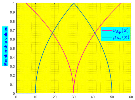
Figure 2. Graph of membership functions of TPFN.

Ranking function: The Rouben’s ranking function [73] of fuzzy numbers is defined as $R_r\left({\mu }_{\tilde{A}}\right)=\frac{1}{2}\left[{\int }_0^1\left(\inf {\tilde{A}}_{\alpha }+\sup {\tilde{A}}_{\alpha }\right)\right]$, where ${\tilde{A}}_{\alpha }$ represents the $\alpha$-cut of fuzzy number $\tilde{A}$.

The ranking function of intuitionistic fuzzy with membership function numbers ${\mu }_{\tilde{I}}$ and non-membership function ${\nu }_{\tilde{I}}$ is defined as $R\left(\tilde{I}\right)=\frac{1}{2}\left[R_r\left({\mu }_{\tilde{I}}\right)+R_r\left({\nu }_{\tilde{I}}\right)\right]$.

Definition:

The ranking function of PFN with membership function ${\mu }_{\tilde{I}}$ and non-membership function ${\nu }_{\tilde{I}}$ is defined as ${\nu }_{\tilde{p}}$ is defined as $R\left(\tilde{p}\right)=\frac{1}{2}\left[R_r\left({\mu }_{\tilde{p}}\right)+R_r\left({\nu }_{\tilde{p}}\right)\right]$.

For a TPFN $A_{\tilde{P}}$ ranking function is

$$\begin{array}{c} R\left(A_{\tilde{P}}\right)=\frac{1}{2}\left[R_r\left({\mu }_{A_{\tilde{P}}}\right)+R_r\left({\nu }_{A_{\tilde{P}}}\right)\right]\hfill \\ =\frac{1}{2}\left(\frac{l_1+l_3+l_2}{3}+\frac{l_1^{\prime }+l_3^{\prime }+l_2}{3}\right)\hfill \\ =\frac{1}{6}\left[l_1+l_3+2l_2+l_1^{\prime }+l_3^{\prime }\right]. \hfill \end{array}$$

2.4. Warehouse Model Formulation of FIFO

A lot size $Q_F$ enters into the system, and from the lot size $Q_F-K_F$ units are transported to backorders and from the remaining quantity (i.e., $K_F$) $\tilde{W}$ units are stored in OW, and the remaining quantity $R (=K_F-\tilde{W}$ for $K_F>\tilde{W}$ or else zero) units are kept in RW. The stock level in OW reaches zero at the time $t_1$ due to demand and deterioration, and the inventory level in RW reaches $R^0$ due to deterioration. This is in accordance with the FIFO policy, which states that the items of RW are only exhausted after the things of OW have been consumed. The inventory in RW reaches zero due to demand and degradation at time $t_2$. As shown in Figure 3, shortages occur during the time period $\left(t_2,T\right)$ and the reorder quantity for the next replenishment is $Q_F=K_F+D_{o}M\left(T-t_2\right)$.

Figure 3. FIFO policy depicted visually.

According to the above FIFO model, the inventory level of OW in the period $\left(0,t_1\right)$ decreases due to both deterioration and demand. To reduce the deterioration of items, this model arranges extra preservation facilities in OW. The inventory level of OW in the interval $\left(0,t_1\right)$ is described by the differential equation follows.

$$\frac{d{I}_o\left(t\right)}{dt}+{\theta }_1\left({\theta }_o,\xi \right)I_o\left(t\right)=-D_{o}M for 0\le t\le t_1,$$

(1)

where $M=\left(a_1{\overline{P}}^{-\delta }{A}^{\gamma }+a_2\mu -a_3\nu \right).$ The solution using the initial condition $I_o\left(0\right)=\tilde{W}$ is

$$I_o\left(t\right)=\left(\tilde{W}+\frac{D_{o}M}{{\theta }_1\left({\theta }_o,\xi \right)}\right)e^{-{\theta }_1\left({\theta }_o,\xi \right)t}-\frac{D_{o}M}{{\theta }_1\left({\theta }_o,\xi \right)} for 0\le t\le t_1,$$

(2)

noting that at $t=t_1$, $I_o\left(t\right)=0$, we get

$$t_1=\frac{1}{{\theta }_1\left({\theta }_o,\xi \right)}\log \left(1+\frac{\tilde{W}{\theta }_1\left({\theta }_o,\xi \right)}{D_{o}M}\right).$$

(3)

2.5. LIFO Warehouse Inventory Model Formulation

A lot size $Q_L$ is introduced into the system and from there, $Q_L-K_L$ units are sent to backorders. An uncertain amount $\tilde{W}$ units are maintained in the OW from the leftover quantity, and $R (=K_L-\tilde{W}$ for $K_L>\tilde{W}$ or zero) is kept in the RW. The initial inventory level is $K_L$ at time $t=0$. The items of the OW are exhausted in accordance with the LIFO policy only after being consumed by the items in the RW and at the time $t_1$ the inventory level in the RW has been depleted owing to demand and deterioration. The OW’s inventory level reaches ${\tilde{W}}^0$ owing to deterioration. Due to demand and decay, the inventory in OW reaches zero at the time $t_2$. The shortages occurring during the period $\left(t_2,T\right)$ and the reorder quantity for the next replenishment are $Q_L=K_L+D_{o}M\left(T-t_2\right)$, the concept of the LIFO policy is depicted visually in Figure 4.

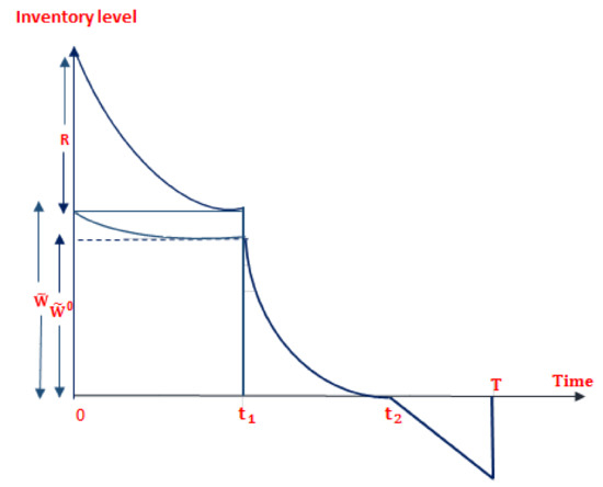
Figure 4. Concept of LIFO policy depicted visually.

According to the above LIFO model, the inventory level of RW in the time period $\left(0,t_1\right)$ decreases due to both deterioration and demand. To reduce the rate of deterioration of commodities, this model includes extra preservation facilities for RW, and therefore, the inventory level of RW may be described by the differential equation within the interval $\left(0,t_1\right)$.

$$\frac{d{I}_r\left(t\right)}{dt}+{\theta }_2\left({\theta }_r,\xi \right)I_r\left(t\right)=-D_{o}M for 0\le t\le t_1.$$

(4)

Using the initial condition $I_r\left(0\right)=R$, we get

$$I_r\left(t\right)=\left(R+\frac{D_{o}M}{{\theta }_2\left({\theta }_r,\xi \right)}\right)e^{-{\theta }_2\left({\theta }_r,\xi \right)t}-\frac{D_{o}M}{{\theta }_2\left({\theta }_r,\xi \right)} for 0\le t\le t_1.$$

(5)

Noting that $I_r\left(t_1\right)=0$, we get

$$t_1=\frac{1}{{\theta }_2\left({\theta }_r,\xi \right)}\log \left(1+\frac{R{\theta }_2\left({\theta }_r,\xi \right)}{D_{o}M}\right).$$

(6)

3. Analysis of Green Warehouse Inventory System

Figure 5 provides a graphical representation of the two-warehouse inventory system, which has been explored under the two discharge policies of FIFO and LIFO.

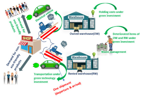
Figure 5. Warehouse inventory system under a green environment.

3.1. Model Formulation of FIFO

The holding cost of commodities in OW during $\left(0,t_1\right)$ is computed as

$$H{C}_{ow}={\int }_0^{t_1} {\overline{h}}_o{I}_o\left(t\right)dt={\overline{h}}_o\left(\frac{\tilde{W}-D_{o}M{t}_1}{{\theta }_1\left({\theta }_o,\xi \right)}\right).$$

(7)

Now, throughout the period $\left(0,t_1\right)$, all of the R units stored in RW are left unused but are susceptible to degradation at the rate of ${\theta }_r$. The sole reason the inventory level in RW decreases to $R^0$ is because of deterioration; therefore, preservation technology is implemented to reduce deterioration and the amount of waste produced. The differential equation describing the state of inventory of RW incorporating preservation in $\left(0,t_1\right)$ is given by:

$$\frac{d{I}_r\left(t\right)}{dt}+{\theta }_2\left({\theta }_r,\xi \right)I_r\left(t\right)=0 for 0\le t\le t_1.$$

(8)

The solution using $I_r\left(0\right)=R$ as boundary condition is given

$$I_r\left(t\right)=R{e}^{-{\theta }_2\left({\theta }_r,\xi \right)t} for 0\le t\le t_1.$$

(9)

Noting that at $t=t_1$, $I_r\left(t_1\right)=R^0$ we get,

$$R^0=R{e}^{-{\theta }_2\left({\theta }_r,\xi \right)t_1}.$$

(10)

For the period $\left(0,t_1\right)$, the holding cost of commodities in RW is calculated as

$${\int }_0^{t_1} {\overline{h}}_r{I}_r\left(t\right)dt={\overline{h}}_r\frac{\left(R-R^0\right)}{{\theta }_2\left({\theta }_r,\xi \right)}.$$

(11)

Again, during a time interval $\left(t_1,t_2\right)$, the quantity available in RW declines due to both demand and degradation, and this study proposed additional preservation facilities to RW also, then the following differential equation that describes the current stock of RW in $\left(t_1,t_2\right)$ is given by:

$$\frac{d{I}_r\left(t\right)}{dt}+{\theta }_2\left({\theta }_r,\xi \right)I_r\left(t\right)=-D_{o}M, t_1\le t\le t_2.$$

(12)

The solution incorporates the boundary condition $I_r\left(t_1\right)=R^0$ is

$$I_r\left(t\right)=\frac{-D_{o}M}{{\theta }_2\left({\theta }_r,\xi \right)}+\left(R^0+\frac{D_{o}M}{{\theta }_2\left({\theta }_r,\xi \right)}\right)e^{{\theta }_2\left({\theta }_r,\xi \right)\left(t_1-t\right)}, t_1\le t\le t_2.$$

(13)

Noting this fact $I_r\left(t_2\right)=0$ and $t^{\ast }=t_2-t_1$, we get

$$t^{\ast }=\frac{1}{{\theta }_2\left({\theta }_r,\xi \right)}log\left(1+\frac{R^0{\theta }_2\left({\theta }_r,\xi \right)}{D_{o}M}\right).$$

(14)

The expense of holding goods owned by RW over the period $\left(t_1,t_2\right)$ is

$${\int }_{t_1}^{t_2} {\overline{h}}_r{I}_r\left(t\right)dt={\overline{h}}_r\left(\frac{R^0-D_{o}M{t}^{\ast }}{{\theta }_2\left({\theta }_r,\xi \right)}\right).$$

(15)

Therefore, the cost of keeping commodities in the RW can be expressed as

$$H{C}_{rw}=\frac{{\overline{h}}_r}{{\theta }_2\left({\theta }_r,\xi \right)}\left[R-D_{o}M{t}^{\ast }\right].$$

(16)

The ordering cost, including the transportation cost of the inventory in the FIFO policy is

$$OC=\eta \left({\overline{C}}_0+2d{t}_v{C}_1+d{t}_v{C}_{2}m{Q}_F\right).$$

(17)

During the shortage period $\left(t_2,T\right)$, the need at any particular time t is fully backlogged. As a result, the shortfall level denoted by S(t) in the scarcity period $\left(t_2,T\right)$ satisfies the differential equation as follows:

$$\frac{dS\left(t\right)}{dt}=-D_{o}M, t_2\le t\le T.$$

The solution by imposing the boundary condition $S\left(t_2\right)=0$ is

$$S\left(t\right)=D_{o}M\left(t_2-t\right), t_2\le t\le T.$$

(18)

Therefore, the shortage cost during the period $\left(t_2,T\right)$ is

$$SC=-{\int }_{t_2}^T {\overline{C}}_{3}S\left(t\right)dt={\overline{C}}_3{D}_{o}M\frac{{(T-t_2)}^2}{2}.$$

(19)

The formula gives the quantity worsened (QW) throughout the period: $QW=\left[K_F-D_{o}M{t}_2\right].$

Therefore, based on the quantity worsened in the period, the deterioration cost (DC) per cycle is

$$DC={\overline{C}}_4\left[K_F-D_{o}M{t}_2\right].$$

(20)

The warehouse inventory management estimates account for the goods’ purchase cost (PC) as follows:

$$PC={\overline{C}}_5{Q}_F={\overline{C}}_5\left[K_F+D_{o}M\left(T-t_2\right)\right].$$

(21)

This research added extra preservation facilities in both OW and RW; for that, invested some money, so the preservation investment cost in both OW and RW per cycle is given by

$$PIC=\xi T.$$

(22)

This study invested some money in making greenhouse inventory, so the green investment cost in both OW and RW per cycle is given by

$$GIC=GT.$$

(23)

3.2. Cost Associated with Carbon Emission in FIFO Policy

It is a typical occurrence that the quantity of carbon emissions varies on the weight that the transporter is carrying. The amount of carbon emissions released by the transportation of empty truck is ${\overline{e}}_{11}$ and weighted truck is ${\overline{e}}_{12}$ multiplied by distance, and the quantity is $\eta \left(2d{\overline{e}}_{11}+d{\overline{e}}_{12}{Q}_F\right)$ units. Here, 2d represents the distance that was also computed for the return trip.

The amount of carbon emissions released for holding items in OW is ${\overline{e}}_2$ multiplied by the total inventory holding area is $\frac{{\overline{e}}_2}{{\theta }_1\left({\theta }_o,\xi \right)}\left[\tilde{W}-D_{o}M{t}_1\right]$ units.

The amount of carbon emissions released for holding items in RW is ${\overline{e}}_3$ multiplied by the total inventory holding area is $\frac{{\overline{e}}_3}{{\theta }_2\left({\theta }_r,\xi \right)}\left[R-D_{o}M{t}^{\ast }\right]$ units.

The amount of carbon emissions released by deteriorating items is ${\overline{e}}_4$ units multiplied by total decaying items is ${\overline{e}}_4\left[K_F-D_{o}M{t}_2\right]$ units.

As a result, the entire quantity of carbon emission ($CE$) produced throughout a cycle is

$$\begin{gathered} CE=\eta \left(2d{\overline{e}}_{11}+d{\overline{e}}_{12}{Q}_F\right)+\frac{{\overline{e}}_2}{{\theta }_1\left({\theta }_o,\xi \right)}\left[\tilde{W}-D_{o}M{t}_1\right] \\ +\frac{{\overline{e}}_3}{{\theta }_2\left({\theta }_r,\xi \right)}\left[R-D_{o}M{t}^{\ast }\right]+{\overline{e}}_4\left[K_F-D_{o}M{t}_2\right]. \end{gathered}$$

(24)

Let $\overline{\varphi }$ be the penalty per unit of carbon emission, then the total emission cost is

$$\begin{array}{c}EC=\hfill \\ \overline{\varphi }CE=\overline{\varphi }\left(\eta \left[2d{\overline{e}}_{11}+d{\overline{e}}_{12}{Q}_F\right]+\frac{{\overline{e}}_2\left(\tilde{W}-D_{o}M{t}_1\right)}{{\theta }_1\left({\theta }_o,\xi \right)}+\frac{{\overline{e}}_3\left(R-D_{o}M{t}^{\ast }\right)}{{\theta }_2\left({\theta }_r,\xi \right)}+{\overline{e}}_4\left[K_F-D_{o}M{t}_2\right]\right).\hfill \end{array}$$

(25)

Now, the parametric form of the interval number is used for the interval-valued parameters [74]. The interval-valued function in parametric form for the interval $\overline{a}$ = $\left[a_L,a_R\right]$ where $a_L>0,a_R>0$ is defined by $\tilde{a}$ =$a\left(\lambda \right)$ = $a_L^{1-\lambda }{a}_R^{\lambda }$, for $\lambda \in \left[0,1\right].$ Using the parametric form for interval-valued numbers and ranking function of fuzzy numbers, the proposed warehouse-inventory system’s total cost is converted into a crisp valued total average cost function.

The total average cost function with emission under defuzzified and parametric parameters per unit time to the system is $TA{C}_F\left(K_F,T\right)$, the following expression gives it:

$$\begin{gathered} TA{C}_F\left(K_F,T\right)=\frac{1}{T}[DC+PC+OC+H{C}_{ow}+H{C}_{rw}+SC \\ +PIC+GIC+Ag+\left(1-F\right)EC]. \end{gathered}$$

(26)

After substituting Equations (7), (16), (17), (19)–(23) and (25) into Equation (26) gives $TA{C}_F\left(K_F,T\right)$ is a function of the continuous variables $K_F$ and T, which provides us to evaluate the total average cost of the warehouse inventory system per unit of time as given below:

$$\begin{array}{c}TA{C}_F\left(K_F,T\right)=\frac{1}{T}[{\tilde{C}}_5\left[K_F+D_{o}M\left(T-t_2\right)\right]+\left\{{\tilde{C}}_4+\left(1-F\right)\tilde{\varphi }{\tilde{e}}_4\right\}\left[K_F-D_{o}M{t}_2\right]\hfill \\ +\eta \left({\tilde{C}}_0+2d{t}_{\nu }{C}_1+d{t}_{\nu }{C}_{2}m{Q}_F\right)+\frac{\left\{{\tilde{h}}_o+\left(1-F\right)\tilde{\varphi }{\tilde{e}}_2\right\}}{{\theta }_1\left({\theta }_o,\xi \right)}\left[\tilde{W}-D_{o}M{t}_1\right]\hfill \\ +\frac{({\tilde{h}}_r+\left(1-F\right)\overline{\varphi }{\tilde{e}}_3}{{\theta }_2\left({\theta }_r,\xi \right)}\left[R-D_{o}M{t}^{\ast }\right]-{\tilde{C}}_3{D}_{o}M\frac{{(T-t_2)}^2}{2}+Ag+GT\hfill \\ +\xi T+\left(1-F\right)\tilde{\varphi }\eta \left\{2d{\tilde{e}}_{11}+d{\tilde{e}}_{12}\left[K_F+D_{o}M\left(T-t_2\right)\right]\right\}].\hfill \end{array}$$

(27)

As $t_2=t_1+t^{\ast }$, after substituting these values, we get,

$$\begin{array}{c}TA{C}_F\left(K_F,T\right)=\frac{1}{T}[\left({\tilde{C}}_5+\eta d{t}_{\nu }{C}_{2}m\right)\left(K_F+D_{o}M\left(T-t_2\right)\right)+\eta \left({\tilde{C}}_0+2d{t}_{\nu }{C}_1\right)\hfill \\ +\left\{{\tilde{C}}_4+\left(1-F\right)\tilde{\varphi }{\tilde{e}}_4\right\}\{K_F-D_{o}M(\frac{1}{{\theta }_1\left({\theta }_o,\xi \right)}\log \left(1+\frac{\tilde{W}{\theta }_1\left({\theta }_o,\xi \right)}{D_{o}M}\right)\hfill \\ +\frac{1}{{\theta }_2\left({\theta }_r,\xi \right)}\log \left(1+\frac{R^0{\theta }_2\left({\theta }_r,\xi \right)}{D_{o}M}\right))\}+\frac{\left\{{\tilde{h}}_o+\left(1-F\right)\tilde{\varphi }{\tilde{e}}_2\right\}}{{\theta }_1\left({\theta }_o,\xi \right)}\hfill \\ \left\{\tilde{W}-\frac{D_{o}M}{{\theta }_1\left({\theta }_o,\xi \right)}\log \left(1+\frac{\tilde{W}{\theta }_1\left({\theta }_o,\xi \right)}{D_{o}M}\right)\right\}+\frac{{\tilde{C}}_3{D}_{o}M}{2}\{T-(\frac{1}{{\theta }_1\left({\theta }_o,\xi \right)}\hfill \\ \log \left(1+\frac{\tilde{W}{\theta }_1\left({\theta }_o,\xi \right)}{D_{o}M}\right)+\frac{1}{{\theta }_2\left({\theta }_r,\xi \right)}log\left(1+\frac{R^0{\theta }_2\left({\theta }_r,\xi \right)}{D_{o}M}\right)){\}}^2\hfill \\ +\frac{\{({\tilde{h}}_r+\left(1-F\right)\tilde{\varphi }{\tilde{e}}_3\}}{{\theta }_2\left({\theta }_r,\xi \right)}\left\{K_F-\tilde{W}-\frac{D_{o}M}{{\theta }_2\left({\theta }_r,\xi \right)}log\left(1+\frac{R^0{\theta }_2\left({\theta }_r,\xi \right)}{D_{o}M}\right)\right\}\hfill \\ +\left(1-F\right)\tilde{\varphi }\eta \left\{2d{\tilde{e}}_{11}+d{\tilde{e}}_{12}\left(K_F+D_{o}M\left(T-t_2\right)\right)\right\}+GT+\xi T+Ag].\hfill \end{array}$$

(28)

3.3. LIFO Model Formulation

The cost of holding materials in RW throughout the period $\left(0,t_1\right)$ is

$$H{C}_{rw}={\int }_0^{t_1} {\overline{h}}_r{I}_r\left(t\right)dt=\frac{{\overline{h}}_r}{{\theta }_2\left({\theta }_r,\xi \right)}\left[R-D_{o}M{t}_1\right].$$

(29)

Now, during the time span $\left(0,t_1\right)$ all the $\tilde{W}$ units in OW are kept unutilized, although they are subject to worsening with a rate of ${\theta }_o$. Thus, OW’s inventory level drops to ${\tilde{W}}^0$ due to degradation alone. The following differential equation reflects the condition of OW’s stock incorporating extra preservation facilities:

$$\frac{d{I}_o\left(t\right)}{dt}+{\theta }_1\left({\theta }_o,\xi \right)I_o\left(t\right)=0 for 0\le t\le t_1.$$

(30)

The solution after applying the boundary constraint $I_o\left(0\right)=\tilde{W}$ is

$$I_o\left(t\right)=\tilde{W}{e}^{-{\theta }_1\left({\theta }_o,\xi \right)t},0\le t\le t_1.$$

(31)

Since $I_o\left(t_1\right)={\tilde{W}}^0$, therefore we get

$${\tilde{W}}^0=\tilde{W}{e}^{-{\theta }_1\left({\theta }_o,\xi \right)t_1}.$$

(32)

The holding cost of commodities in OW in the period $\left(0,t_1\right)$ is

$${\int }_0^{t_1} {\overline{h}}_o{I}_o\left(t\right)dt=\frac{{\overline{h}}_o}{{\theta }_1\left({\theta }_o,\xi \right)}\left(\tilde{W}-{\tilde{W}}^0\right).$$

(33)

Again, during the period $\left(t_1,t_2\right)$, for the reason of demand and deterioration, the commodities in OW decline. Retailer included extra preservation facilities in OW to slow down the deterioration of items. The following differential equation provides the state of the OW inventory during that period is:

$$\frac{d{I}_o\left(t\right)}{dt}+{\theta }_1\left({\theta }_o,\xi \right)I_o\left(t\right)=-D_{o}M, t_1\le t\le t_2.$$

(34)

Incorporating the system boundary condition $I_o\left(t_1\right)={\tilde{W}}^0,$the solution is

$$I_o\left(t\right)=\frac{-D_{o}M}{{\theta }_1\left({\theta }_o,\xi \right)}+\left({\tilde{W}}^0+\frac{D_{o}M}{{\theta }_1\left({\theta }_o,\xi \right)}\right)e^{{\theta }_1\left({\theta }_o,\xi \right)\left(t_1-t\right)} for t_1\le t\le t_2.$$

(35)

Noting that $I_o\left(t_2\right)=0$ and $t^{\ast }=t_2-t_1$ we get

$$t^{\ast }=\frac{1}{{\theta }_1\left({\theta }_o,\xi \right)}log\left(1+\frac{{\tilde{W}}^0{\theta }_1\left({\theta }_o,\xi \right)}{D_{o}M}\right).$$

(36)

The holding amount in OW during the time interval $\left(t_1,t_2\right)$ is

$${\int }_{t_1}^{t_2} {\overline{h}}_o{I}_o\left(t\right)dt=\frac{{\overline{h}}_o}{{\theta }_1\left({\theta }_o,\xi \right)}\left[{\tilde{W}}^0-D_{o}M{t}^{\ast }\right].$$

(37)

Therefore, the holding cost of commodities in the OW is

$$H{C}_{ow}=\frac{{\overline{h}}_o}{{\theta }_1\left({\theta }_o,\xi \right)}\left[\tilde{W}-D_{o}M{t}^{\ast }\right].$$

(38)

The ordering cost, including the transportation cost of the inventory in the LIFO policy, is

$$OC=\eta \left({\overline{C}}_0+2d{t}_{\nu }{C}_1+d{t}_{\nu }{C}_{2}m{Q}_L\right).$$

(39)

During the time interval of shortage incurred $\left(t_2,T\right)$, the demand at t is entirely backlogged. Hence, the shortage level S(t) in OW in that period is concerned with the differential equation:

$$\frac{dS\left(t\right)}{dt}=-D_{o}M, t_2\le t\le T.$$

(40)

Applying $S\left(t_2\right)=0$ as a boundary condition; the solution is $S\left(t\right)=D_{o}M\left(t_2-t\right), t_2\le t\le T.$ Therefore, the shortage cost (SC) in the period $\left(t_2,T\right)$ is

$$SC={\int }_{t_2}^T {\overline{C}}_{3}S\left(t\right)dt={\overline{C}}_3{D}_{o}M\frac{{(T-t_2)}^2}{2}.$$

(41)

The deteriorated amount that occurred throughout the given period is $D=\left[K_L-D_{o}M{t}_2\right].$ The deterioration cost per cycle is given by

$$DC={\overline{C}}_4\left[K_L-D_{o}M{t}_2\right].$$

(42)

The purchasing cost of the items is given as

$$PC={\overline{C}}_5{Q}_L={\overline{C}}_5\left[K_L+D_{o}M\left(T-t_2\right)\right].$$

(43)

To reduce the deterioration rate of stored items, the investment of money is required to improve the technical facilities to incorporate preservation technology. Therefore the preservation investment cost in both OW and RW per cycle is given by

$$PIC=\xi T.$$

(44)

The investment is required for making an eco-friendly depository to incorporate green technology, then the green investment cost of OW and RW per cycle is given by

$$GIC=GT.$$

(45)

3.4. Cost Associated with Carbon Emission in LIFO Policy

The amount of carbon emissions released for transportation of empty truck is ${\overline{e}}_{11}$ and weighted truck is ${\overline{e}}_{12}$, the total emission is $\eta \left(2d{\overline{e}}_{11}+d{\overline{e}}_{12}{Q}_L\right)$ units evaluated by multiplying distance, the number of shipments and quantity.

The amount of carbon emissions released for holding items in OW is ${\overline{e}}_2$ multiplied by the total inventory holding area is $\frac{{\overline{e}}_2}{{\theta }_1\left({\theta }_o,\xi \right)}\left[\tilde{W}-D_{o}M{t}^{\ast }\right]$ units.

The amount of carbon emissions released for holding items in RW is ${\overline{e}}_3$ multiplied by the total inventory holding area is $\frac{{\overline{e}}_3}{{\theta }_2\left({\theta }_r,\xi \right)}\left[R-D_{o}M{t}_1\right]$ units.

The amount of carbon emissions released by deteriorating items is ${\overline{e}}_4$ units multiplied by total decaying items is ${\overline{e}}_4\left[K_L-D_{o}M{t}_2\right]$ units.

Therefore, the total amount of carbon emitted (CE) in a cycle is given by

$$\begin{gathered} CE=\eta \left(2d{\overline{e}}_{11}+d{\overline{e}}_{12}{Q}_L\right)+\frac{{\overline{e}}_2}{{\theta }_1\left({\theta }_o,\xi \right)}\left[\tilde{W}-D_{o}M{t}^{\ast }\right] \\ +\frac{{\overline{e}}_3}{{\theta }_2\left({\theta }_r,\xi \right)}\left[R-D_{o}M{t}_1\right]+{\overline{e}}_4\left[K_L-D_{o}M{t}_2\right]. \end{gathered}$$

(46)

The regulatory body enforces fines for carbon emissions based on the amount of release; therefore, the total emission cost incorporating the imposed penalty $\overline{\varphi }$ is

$$\begin{array}{c}EC=\overline{\varphi }CE\hfill \\ =\overline{\varphi }(\eta \left[2d{\overline{e}}_{11}+d{\overline{e}}_{12}\left(K_L+D_{o}M\left(T-t_2\right)\right)\right]+{\overline{e}}_2\frac{1}{{\theta }_1\left({\theta }_o,\xi \right)}\left[\tilde{W}-D_{o}M{t}^{\ast }\right]\hfill \\ +{\overline{e}}_3\frac{1}{{\theta }_2\left({\theta }_r,\xi \right)}\left[R-D_{o}M{t}_1\right]+{\overline{e}}_4\left[K_L-D_{o}M{t}_2\right]).\hfill \end{array}$$

(47)

The total average cost function with emission under defuzzified and parametric parameters per unit time, $TA{C}_L\left(K_L,T\right)$ is given by

$$\begin{array}{c}TA{C}_L\left(K_L,T\right)=\frac{1}{T}[DC+PC+H{C}_{ow}+H{C}_{rw}+OC+SC+PIC\hfill \\ +GIC+Ag+\left(1-F\right)EC].\hfill \end{array}$$

(48)

After substituting Equations (29), (38), (39), (41)–(45), and (47) into Equation (48), we can calculate the system’s average cost $TA{C}_L\left(K_L,T\right)$ which is a function of the two continuous variables $K_L$ and $T$, as given below:

$$\begin{array}{c}TA{C}_L\left(K_L,T\right)=\frac{1}{T}[{\tilde{C}}_5\left[K_L+D_{o}M\left(T-t_2\right)\right]+{\tilde{C}}_4\left[K_L-D_{o}M{t}_2\right]+\eta ({\tilde{C}}_0+2d{t}_{\nu }{C}_1\hfill \\ +d{t}_2{C}_{2}m{Q}_L)+\frac{{\tilde{h}}_r}{{\theta }_2\left({\theta }_r,\xi \right)}\left[K_L-\tilde{W}-D_{o}M{t}_1\right]+\frac{{\tilde{h}}_o}{{\theta }_1\left({\theta }_o,\xi \right)}\left(\tilde{W}-D_{o}M{t}^{\ast }\right)\hfill \\ -{\tilde{C}}_3{D}_{o}M\frac{{(T-t_2)}^2}{2}+\tilde{\varphi }\left(1-F\right)(\eta \left[2d{\tilde{e}}_{11}+d{\tilde{e}}_{12}{Q}_L\right]+{\tilde{e}}_2\frac{1}{{\theta }_1\left({\theta }_o,\xi \right)}\left[\tilde{W}-D_{o}M{t}^{\ast }\right]\hfill \\ +{\tilde{e}}_3\frac{1}{{\theta }_2\left({\theta }_r,\xi \right)}\left[R-D_{o}M{t}_1\right]+{\tilde{e}}_4\left[K_L-D_{o}M{t}_2\right])+GT+\xi T+Ag].\hfill \end{array}$$

(49)

As $t_2=t_1+t^{\ast }$, after substituting these values, we get,

$$\begin{array}{c}TA{C}_L\left(K_L,T\right)=\frac{1}{T}[\left({\tilde{C}}_5+\eta d{t}_{\nu }{C}_{2}m\right)\left(K_L+D_{o}M\left(T-t_2\right)\right)+\eta \left({\tilde{C}}_0+2d{t}_{\nu }{C}_1\right)\hfill \\ +\frac{\left\{{\tilde{h}}_o+\left(1-F\right)\tilde{\varphi }{\tilde{e}}_2\right\}}{{\theta }_1\left({\theta }_o,\xi \right)}\left\{\tilde{W}-\frac{D_{o}M}{{\theta }_1\left({\theta }_o,\xi \right)}\log \left(1+\frac{{\tilde{W}}^0{\theta }_1\left({\theta }_o,\xi \right)}{D_{o}M}\right)\right\}\hfill \\ +\left\{{\tilde{C}}_4+\left(1-F\right)\tilde{\varphi }{\tilde{e}}_4\right\}\{K_L-D_{o}M(\frac{1}{{\theta }_2\left({\theta }_r,\xi \right)}\log \left(1+\frac{\left(K_L-\tilde{W}\right){\theta }_2\left({\theta }_r,\xi \right)}{D_{o}M}\right)\hfill \\ +\frac{1}{{\theta }_1\left({\theta }_o,\xi \right)}log\left(1+\frac{{\tilde{W}}^0{\theta }_1\left({\theta }_o,\xi \right)}{D_{o}M}\right))\}+\frac{{\tilde{C}}_3{D}_{o}M}{2}\{T-(\frac{1}{{\theta }_2\left({\theta }_r,\xi \right)}\hfill \\ \log \left(1+\frac{\left(K_L-\tilde{W}\right){\theta }_2\left({\theta }_r,\xi \right)}{D_{o}M}\right)+\frac{1}{{\theta }_1\left({\theta }_o,\xi \right)}log\left(1+\frac{{\tilde{W}}^0{\theta }_1\left({\theta }_o,\xi \right)}{D_{o}M}\right)){\}}^2\hfill \\ +\frac{\left\{{\tilde{h}}_r+\left(1-F\right)\tilde{\varphi }{\tilde{e}}_3\right\}}{{\theta }_2\left({\theta }_r,\xi \right)}\left\{\left(K_L-\tilde{W}\right)-\frac{D_{o}M}{{\theta }_2\left({\theta }_r,\xi \right)}\log \left(1+\frac{\left(K_L-\tilde{W}\right){\theta }_2\left({\theta }_r,\xi \right)}{D_{o}M}\right)\right\}\hfill \\ +\tilde{\varphi }\left(1-F\right)\eta \left\{2d{\tilde{e}}_{11}+d{\tilde{e}}_{12}\left(K_L+D_{o}M\left(T-t_2\right)\right)\right\}+\xi T+GT+Ag].\hfill \end{array}$$

(50)

4. Optimization of Inventory System in Pythagorean Fuzziness

In the proposed study of warehouse inventory management, both the policies FIFO and LIFO have been considered to evaluate the total average cost functions$TA{C}_F\left(K_F,T\right)$ and $TA{C}_L\left(K_L,T\right)$ with emission under defuzzified and parametric parameters employing the following estimates, taking into consideration whether or not they are valid for the applicable expressions.

• $\log \left(1+\frac{\tilde{W}{\theta }_1\left({\theta }_o,\xi \right)}{D_{0}M}\right)$=$\frac{\tilde{W}{\theta }_1\left({\theta }_o,\xi \right)}{D_{0}M}-\frac{1}{2}{(\frac{\tilde{W}{\theta }_1\left({\theta }_o,\xi \right)}{D_{0}M})}^2+\frac{1}{3}{(\frac{\tilde{W}{\theta }_1\left({\theta }_o,\xi \right)}{D_{0}M})}^3\mathrm{I}$, for $\left|\frac{\tilde{W}{\theta }_1\left({\theta }_o,\xi \right)}{D_{0}M}\right|<1$
• $\log \left(1+\frac{R^0{\theta }_2\left({\theta }_r,\xi \right)}{D_{0}M}\right)$=$\frac{R^0{\theta }_2\left({\theta }_r,\xi \right)}{D_{0}M}-\frac{1}{2}{(\frac{R^0{\theta }_2\left({\theta }_r,\xi \right)}{D_{0}M})}^2+\frac{1}{3}(\frac{R^0{\theta }_2\left({\theta }_r,\xi \right)}{D_{0}M}I\mathrm{...}$, for $\left|\frac{R^0{\theta }_2\left({\theta }_r,\xi \right)}{D_{0}M}\right|<1$
• $e^{-{\theta }_2\left({\theta }_r,\xi \right)t_0}=1-{\theta }_2\left({\theta }_r,\xi \right)t_0+\frac{({\theta }_2\left({\theta }_r,\xi \right)t_{0}I}{2}\mathrm{....}$
• Second and higher order terms of ${\theta }_1$, ${\theta }_2$ are negligible as $0<{\theta }_1<1$, $0<{\theta }_2<1$, so ${\theta }_1{\theta }_2<1.$

By using these approximations, we get

$$\begin{array}{c}{t}_1=\frac{\tilde{W}}{D_{0}M}-\frac{{\tilde{W}}^2{\theta }_1\left({\theta }_o,\xi \right)}{2{(D_{o}M)}^2}\hfill \\ , R^0=\left(K_F-\tilde{W}\right)\left(1-\frac{\tilde{W}{\theta }_2\left({\theta }_r,\xi \right)}{D_{0}M}\right), \hfill \\ t^{\ast }=\frac{1}{D_{0}M}\left(K_F-\tilde{W}\right)+\frac{{\tilde{W}}^2{\theta }_2\left({\theta }_r,\xi \right)}{2{(D_{o}M)}^2}-\frac{K_F^2{\theta }_2\left({\theta }_r,\xi \right)}{2{(D_{o}M)}^2}, \hfill \\ t_2=t_1+t^{\ast }=\frac{K_F}{D_{0}M}+\frac{{\tilde{W}}^2{\theta }_2\left({\theta }_r,\xi \right)}{2{(D_{o}M)}^2}-\frac{{\tilde{W}}^2{\theta }_1\left({\theta }_o,\xi \right)}{2{(D_{o}M)}^2}-\frac{K_F^2{\theta }_2\left({\theta }_r,\xi \right)}{2{(D_{o}M)}^2}. \hfill \end{array}$$

Furthermore, considering their validity for the following relevant expressions:

• $\log \left(1+\frac{{\tilde{W}}^0{\theta }_1\left({\theta }_o,\xi \right)}{D_{0}M}\right)$=$\frac{{\tilde{W}}^0{\theta }_1\left({\theta }_o,\xi \right)}{D_{0}M}-\frac{1}{2}{(\frac{{\tilde{W}}^0{\theta }_1\left({\theta }_o,\xi \right)}{D_{0}M})}^2+\frac{1}{3}{(\frac{{\tilde{W}}^0{\theta }_1\left({\theta }_o,\xi \right)}{D_{0}M})}^3\mathrm{..}$ for $\left|\frac{{\tilde{W}}^0{\theta }_1\left({\theta }_o,\xi \right)}{D_{0}M}\right|<1$
• $\log \left(1+\frac{\left(K_L-\tilde{W}\right){\theta }_2\left({\theta }_r,\xi \right)}{D_{0}M}\right)$=$\frac{\left(K_L-\tilde{W}\right){\theta }_2\left({\theta }_r,\xi \right)}{D_{0}M}-\frac{1}{2}{(\frac{\left(K_L-\tilde{W}\right){\theta }_2\left({\theta }_r,\xi \right)}{D_{0}M})}^2+\frac{1}{3}{(\frac{\left(K_L-\tilde{W}\right){\theta }_2\left({\theta }_r,\xi \right)}{I})}^3\mathrm{...}$ for $\left|\frac{\left(K_L-\tilde{W}\right){\theta }_2\left({\theta }_r,\xi \right)}{D_{0}M}\right|<1$
• $e^{-{\theta }_1\left({\theta }_o,\xi \right)t_0}=1-{\theta }_1\left({\theta }_o,\xi \right)t_0+\frac{{({\theta }_1\left({\theta }_o,\xi \right)I)}^2}{2}\mathrm{....}$

Second and higher order terms of ${\theta }_o$, ${\theta }_r$ as $0<{\theta }_1<1$, $0<{\theta }_2<1$, so ${\theta }_1{\theta }_2<1.$ By using these approximations, we get

$$\begin{array}{c}{t}_1=\frac{K_L-\tilde{W}}{D_{0}M}-\frac{{(K_L-\tilde{W})}^2{\theta }_2\left({\theta }_r,\xi \right)}{2{(D_{o}M)}^2}\hfill \\ {\tilde{W}}^0=\tilde{W}-\frac{\tilde{W}{\theta }_1\left({\theta }_o,\xi \right)K_L}{D_{0}M}+\frac{{\tilde{W}}^2{\theta }_1\left({\theta }_o,\xi \right)}{D_{0}M}\hfill \\ t^{\ast }=\frac{\tilde{W}}{D_{0}M}-\frac{K_L\tilde{W}{\theta }_1\left({\theta }_o,\xi \right)}{{(D_{o}M)}^2}+\frac{{\tilde{W}}^2{\theta }_1\left({\theta }_o,\xi \right)}{2{(D_{o}M)}^2}\hfill \\ t_2=t_1+t^{\ast }=\frac{K_L}{D_{0}M}-\frac{{(K_L-\tilde{W})}^2{\theta }_2\left({\theta }_r,\xi \right)}{2{(D_{o}M)}^2}+\frac{{\tilde{W}}^2{\theta }_1\left({\theta }_o,\xi \right)}{2{(D_{o}M)}^2}-\frac{K_L\tilde{W}{\theta }_1\left({\theta }_o,\xi \right)}{{(D_{o}M)}^2}\hfill \end{array}$$

4.1. Procedure for Optimal Solution of FIFO Model

We need to determine the total optimal cost of the two-warehouse inventory system from Equation (28), as well as the optimal value of the decision variables $K_F$ and T. We will go into detail about the optimization problem’s optimality criteria in the following.

If $I\left(t\right)$ is not only differentiable but also strictly convex, then any function of the form $\mathsf{\Gamma }\left(t\right)=\frac{I\left(t\right)}{J\left(t\right)}$, $t\in R^n$ is strictly pseudo-convex, though $J\left(t\right)$ is strictly positive and affine as well. Utilizing the $\mathsf{\Gamma }\left(t\right)$ result, we can demonstrate that the objective function is pseudo-convex.

 Theorem 1. 

If$2T{(D_{o}M)}^2+{\theta }_1\left({\theta }_o,\xi \right){\tilde{W}}^2>6K_F{D}_{o}M,$then the Hessian matrix for$TA{C}_F\left(K_F,T\right)$is always positive definite, and therefore$TA{C}_F\left(K_F,T\right)$reaches the global minimum at the unique point$\left(K_F^{\ast },T^{\ast }\right)$.

 Proof. 

To check the optimality of the FIFO policy-based warehouse-inventory system’s average cost$TA{C}_F\left(K_F,T\right)$which is a function of $K_F$and$T$, let us take $TA{C}_F\left(K_F,T\right)=\frac{I_F\left(K_F,T\right)}{J_F\left(K_F,T\right)}$, where

$$\begin{array}{c}{I}_F\left(K_F,T\right)=[\left({\tilde{C}}_5+\eta d{t}_{\nu }{C}_{2}m\right)\left(K_F+D_{o}M\left(T-t_2\right)\right)+\eta \left({\tilde{C}}_0+2d{t}_{\nu }{C}_1\right)\hfill \\ +\left\{{\tilde{C}}_4+\left(1-F\right)\tilde{\varphi }{\tilde{e}}_4\right\}\{K_F-D_{o}M(\frac{1}{{\theta }_1\left({\theta }_o,\xi \right)}\log \left(1+\frac{\tilde{W}{\theta }_1\left({\theta }_o,\xi \right)}{D_{o}M}\right)\hfill \\ +\frac{1}{{\theta }_2\left({\theta }_r,\xi \right)}\log \left(1+\frac{R^0{\theta }_2\left({\theta }_r,\xi \right)}{D_{o}M}\right))\}+\frac{\left\{{\tilde{h}}_o+\left(1-F\right)\tilde{\varphi }{\tilde{e}}_2\right\}}{{\theta }_1\left({\theta }_o,\xi \right)}\{\tilde{W}-\frac{D_{o}M}{{\theta }_1\left({\theta }_o,\xi \right)}\hfill \\ \log \left(1+\frac{\tilde{W}{\theta }_1\left({\theta }_o,\xi \right)}{D_{o}M}\right)\}+\frac{{\tilde{C}}_3{D}_{o}M}{2}\{T-(\frac{1}{{\theta }_1\left({\theta }_o,\xi \right)}\hfill \\ \log \left(1+\frac{\tilde{W}{\theta }_1\left({\theta }_o,\xi \right)}{D_{o}M}\right)+\frac{1}{{\theta }_2\left({\theta }_r,\xi \right)}log\left(1+\frac{R^0{\theta }_2\left({\theta }_r,\xi \right)}{D_{o}M}\right)){\}}^2\hfill \\ +\frac{\{(h_r+\left(1-F\right)\tilde{\varphi }{\tilde{e}}_3\}}{{\theta }_2\left({\theta }_r,\xi \right)}\left\{K_F-\tilde{W}-\frac{D_{o}M}{{\theta }_2\left({\theta }_r,\xi \right)}log\left(1+\frac{R^0{\theta }_2\left({\theta }_r,\xi \right)}{D_{o}M}\right)\right\}\hfill \\ +\left(1-F\right)\eta \tilde{\varphi }[2d{\tilde{e}}_{11}+d{\tilde{e}}_{12}\left[K_F+D_{o}M\left(T-t_2\right)\right]\left]+GT+\xi T+Ag\right]\hfill \end{array}$$

(51)

and $J_F\left(K_F,T\right)=T$. Then,

$$\begin{gathered} \frac{{\partial }^2{I}_F\left(K_F,T\right)}{\partial K_F^2}=\frac{1}{2{(D_{o}M)}^3}[{\theta }_2^2\left({\theta }_r,\xi \right){\tilde{C}}_3\left(3K_F^2-{\tilde{W}}^2\right)+2{(D_{o}M)}^2\left({\tilde{C}}_3+{\tilde{h}}_r+{\tilde{e}}_3\tilde{\varphi }-{\tilde{e}}_{3}F\tilde{\varphi }\right) \\ +{\theta }_2\left({\theta }_r,\xi \right)({\tilde{C}}_3(-6K_F{D}_{o}M+2T\left(D_{o}M{)}^2+{\theta }_1\left({\theta }_o,\xi \right){\tilde{W}}^2\right) \\ +2\left(D_{o}M{)}^2\left({\tilde{C}}_4+{\tilde{C}}_5+C_{2}dm\eta t_{\nu }+\left(\eta d{\tilde{e}}_{12}+{\tilde{e}}_4\right)\tilde{\varphi }\left(1-F\right)\right)\right)] \end{gathered}$$

(52)

$$\frac{{\partial }^2{I}_F\left(K_F,T\right)}{\partial K_F\partial T}={\tilde{C}}_3\left[-1+\frac{{\theta }_2\left({\theta }_r,\xi \right)K_F}{D_{o}M}\right]$$

(53)

$$\frac{{\partial }^2{I}_F\left(K_F,T\right)}{\partial T\partial K_F}={\tilde{C}}_3\left[-1+\frac{{\theta }_2\left({\theta }_r,\xi \right)K_F}{D_{o}M}\right]$$

(54)

$$\frac{{\partial }^2{I}_F\left(K_F,T\right)}{\partial T^2}={\tilde{C}}_3{D}_{o}M$$

(55)

From Equation (52), we can observe that the value of $\frac{{\partial }^2{I}_F\left(K_F,T\right)}{\partial K_F^2}>0$if the value of ${\tilde{C}}_3(-6K_F{D}_{o}M+2T\left(D_{o}M{)}^2+{\theta }_1\left({\theta }_o,\xi \right){\tilde{W}}^2\right)$ is greater than zero, i.e., $2T{(D_{o}M)}^2+{\theta }_1\left({\theta }_o,\xi \right){\tilde{W}}^2>6K_F{D}_{o}M$.

Let us assume the Hessian matrix of $I_F\left(K_F,T\right)$ is $H_{22}=\left[\begin{array}{cc}\frac{{\partial }^2{I}_F\left(K_F,T\right)}{\partial T^2}& \frac{{\partial }^2{I}_F\left(K_F,T\right)}{\partial T\partial K_F}\\ \frac{{\partial }^2{I}_F\left(K_F,T\right)}{\partial K_F\partial T}& \frac{{\partial }^2{I}_F\left(K_F,T\right)}{\partial K_F^2}\end{array}\right]$.

The first principal minors of $H_{22}$ is $\frac{{\partial }^2{I}_F\left(K_F,T\right)}{\partial T^2}>0$ and the second principal minor of $H_{22}$ is:

$$\begin{array}{c}\left|H_{22}\right|=\left|\begin{array}{cc}\frac{{\partial }^2{I}_F\left(K_F,T\right)}{\partial T^2}& \frac{{\partial }^2{I}_F\left(K_F,T\right)}{\partial T\partial K_F}\\ \frac{{\partial }^2{I}_F\left(K_F,T\right)}{\partial K_F\partial T}& \frac{{\partial }^2{I}_F\left(K_F,T\right)}{\partial K_F^2}\end{array}\right|=\frac{{\partial }^2{I}_F\left(K_F,T\right)}{\partial K_F^2}\frac{{\partial }^2{I}_F\left(K_F,T\right)}{\partial T^2}-\frac{{\partial }^2{I}_F\left(K_F,T\right)}{\partial K_F\partial T}\frac{{\partial }^2{I}_F\left(K_F,T\right)}{\partial T\partial K_F}\hfill \\ =\frac{1}{2{(D_{o}M)}^2}[{\tilde{C}}_3({\theta }_2^2\left({\theta }_r,\xi \right){\tilde{C}}_3\left(K_F^2-{\tilde{W}}^2\right)+2{(D_{o}M)}^2\left(h_r+{\tilde{e}}_3\tilde{\varphi }-{\tilde{e}}_{3}F\tilde{\varphi }\right)\hfill \\ +{\theta }_2\left({\theta }_r,\xi \right)({\tilde{C}}_3(-2K_F{D}_{o}M+2T\left(D_{o}M{)}^2+{\theta }_1\left({\theta }_o,\xi \right){\tilde{W}}^2\right)\hfill \\ +2\left(D_{o}M{)}^2\left({\tilde{C}}_4+{\tilde{C}}_5+C_{2}dm\eta t_{\nu }+\left(\eta d{\tilde{e}}_{12}+{\tilde{e}}_4\right)\tilde{\varphi }\left(1-F\right)\right)\right))]\hfill \end{array}$$

(56)

The second principal minor is greater than zero only if $2T{(D_{o}M)}^2+{\theta }_1\left({\theta }_o,\xi \right){\tilde{W}}^2>2K_F{D}_{o}M.$ If $2T{(D_{o}M)}^2+{\theta }_1\left({\theta }_o,\xi \right){\tilde{W}}^2>6K_F{D}_{o}M$, then obviously $2T{(D_{o}M)}^2+{\theta }_1\left({\theta }_o,\xi \right){\tilde{W}}^2>2K_F{D}_{o}M,$since $2T{(D_{o}M)}^2+{\theta }_1\left({\theta }_o,\xi \right){\tilde{W}}^2>6K_F{D}_{o}M>2K_F{D}_{o}M.$ Therefore, the function $I_F\left(K_F,T\right)$ is strictly convex and differentiable, since $\frac{{\partial }^2{I}_F\left(K_F,T\right)}{\partial T^2}>0$ and$\frac{{\partial }^2{I}_F\left(K_F,T\right)}{\partial K_F^2}>0, \left|H_{22}\right|>0 \mathrm{if} 2T{(D_{o}M)}^2+{\theta }_1\left({\theta }_o,\xi \right){\tilde{W}}^2>6K_F{D}_{o}M$.

In addition, $J_F\left(K_F,T\right)=T$ is a strictly positive and affine function. Using Theorem 3.2.5 in Cambini and Martein [75], $TA{C}_F\left(K_F,T\right)$ achieves the global minimum at a point $\left(K_F^{\ast },T^{\ast }\right),$ which is derived from the necessary conditions. This completes the proof.

4.2. Procedure for Optimal Solution of LIFO Model

We need to determine the total optimal cost of the two-warehouse inventory system from Equation (50), as well as the optimal value of the decision variables $K_{\mathrm{L}}$ and T. We will go into detail about the optimization problem’s optimality criteria in the following.

 Theorem 2. 

The total average cost attains a global minimum at a unique point $\left(K_L^{\ast },T^{\ast }\right)$

if $2T{(D_{o}M)}^2+{\theta }_1\left({\theta }_o,\xi \right)K_L\tilde{W}+{\theta }_1\left({\theta }_o,\xi \right)\mathrm{R}\tilde{W}>2K_L{D}_{o}M$

, then the Hessian matrix for $TA{C}_L\left(K_L,T\right)$

is positive definite.

 Proof. 

To check the optimality of the LIFO policy-based warehouse-inventory system’s average cost $TA{C}_L\left(K_L,T\right)$

which is a function of $K_L$

and $T$, let us take $TA{C}_L\left(K_L,T\right)=\frac{I_L\left(K_L,T\right)}{J_L\left(K_L,T\right)}$

$$\begin{array}{c}\mathrm{where} I_L\left(K_L,T\right)=\frac{1}{T}[\left({\tilde{C}}_5+\eta d{t}_{\nu }{C}_{2}m\right)\left(K_L+D_{o}M\left(T-t_2\right)\right)+\eta \left({\tilde{C}}_0+2d{t}_{\nu }{C}_1\right)\hfill \\ +\frac{\left\{{\tilde{h}}_o+\left(1-F\right)\tilde{\varphi }{\tilde{e}}_2\right\}}{{\theta }_1\left({\theta }_o,\xi \right)}\left\{\tilde{W}-\frac{D_{o}M}{{\theta }_1\left({\theta }_o,\xi \right)}\log \left(1+\frac{{\tilde{W}}^0{\theta }_1\left({\theta }_o,\xi \right)}{D_{o}M}\right)\right\}\hfill \\ +\left\{{\tilde{C}}_4+\left(1-F\right)\tilde{\varphi }{\tilde{e}}_4\right\}\{K_L-D_{o}M(\frac{1}{{\theta }_2\left({\theta }_r,\xi \right)}\log \left(1+\frac{\left(K_L-\tilde{W}\right){\theta }_2\left({\theta }_r,\xi \right)}{D_{o}M}\right)\hfill \\ +\frac{1}{{\theta }_1\left({\theta }_o,\xi \right)}log\left(1+\frac{{\tilde{W}}^0{\theta }_1\left({\theta }_o,\xi \right)}{D_{o}M}\right))\}+\frac{{\tilde{C}}_3{D}_{o}M}{2}\{T-(\frac{1}{{\theta }_2\left({\theta }_r,\xi \right)}\hfill \\ \log \left(1+\frac{\left(K_L-\tilde{W}\right){\theta }_2\left({\theta }_r,\xi \right)}{D_{o}M}\right)+\frac{1}{{\theta }_1\left({\theta }_o,\xi \right)}log\left(1+\frac{{\tilde{W}}^0{\theta }_1\left({\theta }_o,\xi \right)}{D_{o}M}\right)){\}}^2\hfill \\ +\frac{\left\{{\tilde{\tilde{h}}}_r+\left(1-F\right)\tilde{\varphi }{\tilde{e}}_3\right\}}{{\theta }_2\left({\theta }_r,\xi \right)}\left\{\left(K_L-\tilde{W}\right)-\frac{D_{o}M}{{\theta }_2\left({\theta }_r,\xi \right)}\log \left(1+\frac{\left(K_L-\tilde{W}\right){\theta }_2\left({\theta }_r,\xi \right)}{D_{o}M}\right)\right\}\hfill \\ +\tilde{\varphi }\left(1-F\right)\eta \left\{2d{\tilde{e}}_{11}+d{\tilde{e}}_{12}\left(K_L+D_{o}M\left(T-t_2\right)\right)+\xi T+GT+Ag\right\}]\hfill \end{array}$$

(57)

and $J_L\left(K_L,T\right)=T$. Then,

$$\begin{array}{c}\frac{{\partial }^2{I}_L\left(K_L,T\right)}{\partial K_L^2}=\frac{1}{2{(D_{o}M)}^3}[3{\theta }_2^2\left({\theta }_r,\xi \right){\tilde{C}}_3{(K_L-\tilde{W})}^2+2({\tilde{C}}_3{(D_{o}M-{\theta }_1\left({\theta }_o,\xi \right)\tilde{W})}^2\hfill \\ +\left(D_{o}M{)}^2\left({\tilde{h}}_r+{\tilde{e}}_3\tilde{\varphi }-{\tilde{e}}_{3}F\tilde{\varphi }\right)\right)+{\theta }_2\left({\theta }_r,\xi \right)({\tilde{C}}_3(-6K_L{D}_{o}M+2T{(D_{o}M)}^2\hfill \\ +6{\theta }_1\left({\theta }_o,\xi \right)K_L\tilde{W}+4D_{o}M\tilde{W}-5{\theta }_1\left({\theta }_o,\xi \right){\tilde{W}}^2)\hfill \\ +2\left(D_{o}M{)}^2\left({\tilde{C}}_4+{\tilde{C}}_5+C_{2}dm\eta t_{\nu }+\left(\eta d{\tilde{e}}_{12}+{\tilde{e}}_4\right)\tilde{\varphi }\left(1-F\right)\right)\right)]\hfill \end{array}$$

(58)

$$\frac{{\partial }^2{I}_L\left(K_L,T\right)}{\partial K_L\partial T}=\frac{{\tilde{C}}_3}{D_{o}M}\left[-D_{o}M+{\theta }_2\left({\theta }_r,\xi \right)\left(K_L-\tilde{W}\right)+{\theta }_1\left({\theta }_o,\xi \right)\tilde{W}\right],$$

(59)

$$\frac{{\partial }^2{I}_L\left(K_L,T\right)}{\partial T\partial K_L}=\frac{{\tilde{C}}_3}{D_{o}M}\left[-D_{o}M+{\theta }_2\left({\theta }_r,\xi \right)\left(K_L-\tilde{W}\right)+{\theta }_1\left({\theta }_o,\xi \right)\tilde{W}\right]$$

(60)

$$\frac{{\partial }^2{I}_L\left(K_L,T\right)}{\partial T^2}={\tilde{C}}_3{D}_{o}M.$$

(61)

Simple observation reveals that the value $\frac{{\partial }^2{I}_L\left(K_L,T\right)}{\partial K_L^2}>0$ always if ${\theta }_2\left({\theta }_r,\xi \right)({\tilde{C}}_3(-6K_L{D}_{o}M+2T\left(D_{o}M{)}^2+6{\theta }_1\left({\theta }_o,\xi \right)K_L\tilde{W}+4D_{o}M\tilde{W}-5{\theta }_1\left({\theta }_o,\xi \right){\tilde{W}}^2\right)$>0. i.e., $2T{(D_{o}M)}^2+{\theta }_1\left({\theta }_o,\xi \right)K_L\tilde{W}+5{\theta }_1\left({\theta }_o,\xi \right)\mathrm{R}\tilde{W}>2D_{o}M\left(K_L\right)+4\mathrm{R}{D}_{o}M$.

Now, Hessian matrix $H_{22}=\left[\begin{array}{cc}\frac{{\partial }^2{I}_L\left(K_L,T\right)}{\partial T^2}& \frac{{\partial }^2{I}_L\left(K_L,T\right)}{\partial T\partial K_L}\\ \frac{{\partial }^2{I}_L\left(K_L,T\right)}{\partial K_L\partial T}& \frac{{\partial }^2{I}_L\left(K_L,T\right)}{\partial K_L^2}\end{array}\right]$.

The first principal minors of $H_{22}$ is $\frac{{\partial }^2{I}_L\left(K_L,T\right)}{\partial T^2}>0$ and the second principal minor of $H_{22}$ is:

$$\begin{array}{c}\left|H_{22}\right|=\left|\begin{array}{cc}\frac{{\partial }^2{I}_L\left(K_L,T\right)}{\partial T^2}& \frac{{\partial }^2{I}_L\left(K_L,T\right)}{\partial T\partial K_L}\\ \frac{{\partial }^2{I}_L\left(K_L,T\right)}{\partial K_L\partial T}& \frac{{\partial }^2{I}_L\left(K_L,T\right)}{\partial K_L^2}\end{array}\right|=\frac{{\partial }^2{I}_L\left(K_L,T\right)}{\partial K_L^2}\frac{{\partial }^2{I}_L\left(K_L,T\right)}{\partial T^2}-\frac{{\partial }^2{I}_L\left(K_L,T\right)}{\partial K_L\partial T}\frac{{\partial }^2{I}_L\left(K_L,T\right)}{\partial T\partial K_L}\hfill \\ =\frac{{\tilde{C}}_3}{2{(D_{o}M)}^2}[{\theta }_2^2\left({\theta }_r,\xi \right){\tilde{C}}_3{(K_L-\tilde{W})}^2+2{(D_{o}M)}^2\left({\tilde{h}}_r+{\tilde{e}}_3\tilde{\varphi }-{\tilde{e}}_{3}F\tilde{\varphi }\right)\hfill \\ +{\theta }_2\left({\theta }_r,\xi \right)({\tilde{C}}_3(-2K_L{D}_{o}M+2T\left(D_{o}M{)}^2-{\theta }_1\left({\theta }_o,\xi \right){\tilde{W}}^2+2{\theta }_1\left({\theta }_o,\xi \right)\tilde{W}{K}_L\right)\hfill \\ +2\left(D_{o}M{)}^2\left({\tilde{C}}_4+{\tilde{C}}_5+C_{2}dm\eta t_{\nu }+\left(\eta d{\tilde{e}}_{12}+{\tilde{e}}_4\right)\tilde{\varphi }\left(1-F\right)\right)\right))]\hfill \end{array}$$

(62)

The second principal minor is greater than zero only if $(-2K_L{D}_{o}M+2T\left(D_{o}M{)}^2-{\theta }_1\left({\theta }_o,\xi \right){\tilde{W}}^2+2{\theta }_1\left({\theta }_o,\xi \right)\tilde{W}{K}_L\right)>0$i.e., $2T{(D_{o}M)}^2+{\theta }_1\left({\theta }_o,\xi \right)K_L\tilde{W}+{\theta }_1\left({\theta }_o,\xi \right)\mathrm{R}\tilde{W}>2K_L{D}_{o}M.$ If $2T{(D_{o}M)}^2+{\theta }_1\left({\theta }_o,\xi \right)K_L\tilde{W}+{\theta }_1\left({\theta }_o,\xi \right)\mathrm{R}\tilde{W}>2K_L{D}_{o}M,$ then obviously $2T{(D_{o}M)}^2+{\theta }_1\left({\theta }_o,\xi \right)K_L\tilde{W}+5{\theta }_1\left({\theta }_o,\xi \right)\mathrm{R}\tilde{W}>2D_{o}M\left(K_L\right)+4\mathrm{R}{D}_{o}M,$ since $2T{(D_{o}M)}^2+{\theta }_1\left({\theta }_o,\xi \right)K_L\tilde{W}+5{\theta }_1\left({\theta }_o,\xi \right)\mathrm{R}\tilde{W}>2T{(D_{o}M)}^2+{\theta }_1\left({\theta }_o,\xi \right)K_L\tilde{W}+{\theta }_1\left({\theta }_o,\xi \right)\mathrm{R}\tilde{W}>2D_{o}M\left(K_L\right)>2D_{o}M\left(K_L\right)+4\mathrm{R}{D}_{o}M.$ Therefore, the function $I_F\left(K_F,T\right)$ is strictly convex and differentiable, since $\frac{{\partial }^2{I}_L\left(K_L,T\right)}{\partial T^2}>0$ and$\frac{{\partial }^2{I}_L\left(K_L,T\right)}{\partial K_L^2}>0, \left|H_{22}\right|>0 \mathrm{if} 2T{(D_{o}M)}^2+{\theta }_1\left({\theta }_o,\xi \right)K_L\tilde{W}+{\theta }_1\left({\theta }_o,\xi \right)\mathrm{R}\tilde{W}>2K_L{D}_{o}M$.

The function $J_L\left(K_L,T\right)=T$ is also strictly positive and affine. Now, the Theorem 3.2.5 in Cambini and Martein [75], is used to show that $TA{C}_L\left(K_L,T\right)$ achieves the global minimum value at the specific point $\left(K_L^{\ast },T^{\ast }\right)$ that is obtained from the prerequisites. This completes the proof.

5. Numerical Solution

Case Study of Eco-Friendly Paint Warehouses:

A case study presented here focuses on warehouse management of eco-friendly paints from Indore city. The ideal temperature for storing paints varies depending on the type. In green warehouse systems, controllable deterioration and emission rates for preserving are used to preserve paints for longer. In the present scenario, the demand rate is related to the selling price, advertisement, and usage percentage of herbal and chemical substances to encourage customers to buy eco-friendly paints. This study considers the sustainable inventory models for the order quantity and total green warehouse retailer cost of a green warehouse paint farm in Indore city. Environmentally responsible inventory models are more prevalent. The long-term effects of carbon emissions from transportation on our ecosystem globally make them significant compared to traditional inventory models today. Regarding the model’s applicability, we can say any warehouse firm that comes under the simple carbon tax policy discussed in the paper can adopt the model. The proposed model can be used appropriately in some warehouse sectors, including paint, food, drugs, medicine, etc. The data has been taken from the eco-friendly paint warehouses in Indore city. Most of the input data are carried out directly from the case study. However, some information has been observed as changing in nature, so the study has been conducted by extending those data. The input has been counted as the interval for the selling price ($\overline{P}$), ordering cost (${\overline{C}}_0$), shortages cost (${\overline{C}}_3$), deterioration cost (${\overline{C}}_4$), purchasing cost (${\overline{C}}_5$), holding costs, carbon emission parameters, and taxes.

This section provides a numerical example to understand the presented two-warehouses inventory system by taking the numerical data from Table 2 with additional parameters $a=0.4, b=0.7, a_1=15$, $\delta =0.7$, $a_2=0.25$, $a_3=0.6$, and $\rho =0.$ The numerical simulation of the proposed model was performed in wolfram Mathematica version 9.0 and the sensitivity analysis are performed by using MATLAB software R2022a with 64 bit operating system. Based on the information of retailer, the OW storage capacity of paints is taken as a pentagonal fuzzy number i.e., $\mathrm{W} \text{˜}=\{480,620,860);\left(420,620,900\right)$ units.

Table 2. Numerical data for the given case study.

Parameter	Value
$\mu$	80%
$\nu$	20%
$D_o$	360 units
$A, \gamma$	50, 0.4
$\xi$	$5/unit time
$t_v$	$0.2/L
$C_1$	0.375 L/100 km
$C_2$	0.9 L/100 km/ton of payload
$m$	5 kg/unit
$d$	100 km
$\overline{P}=\left[P_L,P_R\right]$	$\$\left[50,70\right]$/unit item
${\overline{C}}_0=\left[C_{0L},C_{0R}\right]$	$\$\left[50,100\right]$/shipment
${\overline{C}}_3=\left[C_{3L},C_{3R}\right]$	$\$\left[15,25\right]$/unit item/unit time
${\overline{C}}_4=\left[C_{4L},C_{4R}\right]$	$\$\left[5,10\right]$/unit item/unit time
${\overline{C}}_5=\left[C_{5L},C_{5R}\right]$	$\$\left[20,30\right]$/unit item
${\overline{h}}_o=\left[h_{oL},h_{oR}\right]$	$\$\left[1,2\right]$/unit item/unit time
${\overline{h}}_r=\left[h_{rL},h_{rR}\right]$	$\$\left[1,2\right]$/unit item/unit time
${\theta }_o$ ${\theta }_r$	0.2 0.1
$\overline{\varphi }=\left[{\varphi }_L,{\varphi }_R\right]$	$\$\left[0.1,0.6\right]$/kg emission
${\overline{e}}_{11}=\left[e_{11L},e_{11R}\right]$	$\left[5,15\right]$ kg/km
${\overline{e}}_{12}=\left[e_{12L},e_{12R}\right]$ ${\overline{e}}_2=\left[e_{2L},e_{2R}\right]$ ${\overline{e}}_3=\left[e_{3L},e_{3R}\right]$ ${\overline{e}}_4=\left[e_{4L},e_{4R}\right]$	$\left[5,6\right]$ kg/unit/km $\left[3,4\right]$ kg per unit $\left[2,6\right]$ kg per unit $\left[4,5\right]$ kg per unit
$\eta$ $G$ $g$	2 $5/unit time $36

Table 3 shows that the total optimal cost is less under green technology investment. The optimal cycle length and quantity are also more under green technology investment. It concludes a retailer can store more quantity with less cost with green investment. The convex representation of the total average optimal cost under green technology investment is shown in Figure 6 where the filled point in red indicates the location of the optimal solution.

Table 3. Comparison of optimal solution of FIFO and LIFO policies with or without green technology.

Green Environment	${\mathit{t}}_1^{\ast } \left(\mathrm{Year}\right)$	${\mathit{t}}_2^{\ast } \left(\mathrm{Year}\right)$	${\mathit{T}}^{\ast } \left(\mathrm{Year}\right)$	${\mathit{K}}_{\mathit{F}}^{\ast }$	$\mathit{T}\mathit{A}{\mathit{C}}_{\mathit{F}}^{\ast }$	${\mathit{Q}}_{\mathit{F}}^{\ast }$	${\mathit{t}}_1^{\ast } \left(\mathbf{Year}\right)$	${\mathit{t}}_2^{\ast } \left(\mathbf{Year}\right)$	${\mathit{T}}^{\ast } \left(\mathbf{Year}\right)$	${\mathit{K}}_{\mathit{L}}^{\ast }$	$\mathit{T}\mathit{A}{\mathit{C}}_{\mathit{L}}^{\ast }$	${\mathit{Q}}_{\mathit{L}}^{\ast }$
With	0.286347	0.592897	0.736153	1347.32	507257	1671.25	0.183826	0.468740	0.628792	1066.17	507992	1428.08
Without	0.286347	0.510707	0.696300	1160.68	773889	1579.73	0.077260	0.363006	0.565506	824.788	774629	1282.67

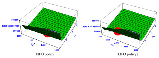
Figure 6. Graphical representation of convexity of a total cost function for FIFO $\mathrm{and}$.

The reduction of emissions is the impact of the specified model’s investment in green technology. This model considers two functions for a fraction of emission reduced under green technology $\left(F\right)$ in this model. The first function is $F=\rho \left(1-e^{-bG}\right)$ and the second function is $F=\rho \left(\frac{bG}{1+bG}\right)$. Table 3 represents the optimal cost of the warehouse inventory system under the various functions of $F$.

Table 4 shows that the total cost under emissions without green technology is higher than that of the total cost under incorporating green technology. With green technology investment, retailer can store more quantities with less cost and a longer replenishment cycle time. The green technology investment for both functions is the same, i.e., G = 5. The results show that the total optimal cost is lower in function-I than in function II, and function I’s replenishment cycle time and quantity are also high. With less green investment, retaile can reduce high emissions for some commodities; function-I is the best choice in those situations. Similarly, for some commodities storing, holding, and transporting, retailer has to invest a high green investment amount and fewer emissions only reduced in those situations; function II is the better choice. For Table 3 and sensitivity analysis, we consider function-I for a fraction of emission reduced under green technology $\left(F\right)$ in this model.

Table 4. Total optimal cost of inventory system under emission and green technology.

		FIFO Policy						LIFO Policy						Suggested Policy
Environment	Deterioration	$K_F^{\ast }$	$T^{\ast }$ (year)	$TA{C}_F^{\ast }$	CE	CE (Green Investment)	Reduction	$K_L^{\ast }$	$T^{\ast }$ (year)	$TA{C}_L^{\ast }$	CE	CE (Green Investment)	Reduction	Policy
Emission	${\theta }_o>{\theta }_r$ ${\theta }_o={\theta }_r$ ${\theta }_o<{\theta }_r$	1160.08 1066.09 684.051	0.696300 0.640437 0.485351	773889 773226 773797	868038 797649 604037	- - -	- - -	824.788 1066.09 914.135	0.565506 0.640437 0.577859	774629 773226 773415	704819 797649 719535	- - -	- - -	FIFO Either LIFO
Emission and Green technology for function-I	${\theta }_o>{\theta }_r$ ${\theta }_o={\theta }_r$ ${\theta }_o<{\theta }_r$	1347.32 1259.77 846.659	0.736153 0.688915 0.523788	507257 506846 507582	918531 858778 652654	116817 109217 83002.9	87 87 87	1066.17 1259.77 1047.65	0.628792 0.688915 0.601486	507992 506846 507106	784820 858778 749576	99811.6 109217 95329.3	57 57 57	FIFO Either LIFO
Emission and Green technology for function-II	${\theta }_o>{\theta }_r$ ${\theta }_o={\theta }_r$ ${\theta }_o<{\theta }_r$	1300.37 1211.06 805.639	0.724381 0.675218 0.512934	560071 559611 560321	903652 841523 638934	271096 252457 191680	70 70 70	1006.92 1211.06 1013.56	0.611978 0.675218 0.593880	560820 559611 559856	763572 841523 739944	229071 252457 221983	70 70 70	FIFO Either LIFO

6. Sensitivity Analysis

We carried out the sensitivity analysis under various holding costs and deterioration rates, and using that the decision-maker could suggest a suitable dispatch policy. By changing parameters from $-20\%$ to $20\%$ to analyze the robustness of the two-warehouse inventory system for parameters under various deterioration rates. In Table 5, we evaluated the optimal cost for the proposed system by considering various holding costs.

Table 5. Optimal cost of inventory system under various holding costs and deterioration rates.

		FIFO Policy			LIFO Policy			Suggested
Environment	$r\left(\frac{{\theta }_o}{{\theta }_r}\right)$	$K_F^{\ast }$	$T^{\ast }$(Year)	$TA{C}_F^{\ast }$	$K_L^{\ast }$	$T^{\ast }$(Year)	$TA{C}_L^{\ast }$	Policy
${\tilde{h}}_o>{\tilde{h}}_r$	0.25 0.5 1 2 4	1251.11 1273.70 1317.71 1401.64 1556.08	0.684607 0.696797 0.720548 0.765801 0.848963	560,805 506,911 507,118 507,512 508,238	1276.47 1232.08 1137.21 918.682 273.551	0.694802 0.681810 0.652626 0.579076 0.320964	506,729 507,033 507,613 508,643 509,733	LIFO FIFO FIFO FIFO FIFO
${\tilde{h}}_o={\tilde{h}}_r$	0.25 0.5 1 2 4	1189.93 1213.65 1259.77 1656.87 1984.58	0.651197 0.664012 0.688915 0.847415 0.980343	506,519 506,630 506,846 506,096 505,554	1384.22 1344.51 1259.77 1491.43 1697.70	0.723131 0.712651 0.688915 0.785490 0.872264	505,893 506,219 506,846 506,605 506,421	LIFO LIFO Either FIFO FIFO
${\tilde{h}}_o<{\tilde{h}}_r$	0.25 0.5 1 2 4	899.411 919.483 958.384 1173.62 1319.40	0.534824 0.546603 0.569422 0.655565 0.713728	507,014 507,149 507,411 507,014 506,729	1199.14 1167.78 1101.47 1212.76 1293.07	0.647761 0.640431 0.623744 0.669721 0.703089	506,160 506,460 507,036 506,900 506,809	LIFO LIFO LIFO LIFO FIFO

From Table 5, the following comments are noted from the proposed system. We considered ${\tilde{h}}_o>{\tilde{h}}_r$, i.e., holding cost of OW is greater than the RW, then we can observe the following facts:

• If $r<1$, i.e., the rate of degradation of OW is lower than the rate of deterioration of RW, the total average cost of FIFO policy is lower than the total average cost of LIFO policy. Therefore, the managerial decision suggests the FIFO policy. However, the LIFO policy has a lower overall average cost than the FIFO approach if $r=0.25$, so the recommended policy is LIFO.
• If $r=1$, i.e., the rate of degradation of OW and RW is the same, then the total cost of the FIFO policy is less than the total cost of the LIFO policy; hence, FIFO is recommended in this scenario.
• If $r>1$, i.e., the OW degradation rate is higher, the advised policy is FIFO because the FIFO policy’s total average cost is lower than the LIFO policy’s total average cost.
• The following observations are made when the holding costs of RW and OW are the same, i.e., ${\tilde{h}}_o={\tilde{h}}_r$:
• If $r<1$, i.e., the rate of deterioration of OW is lower than RW and the overall average cost is lower for LIFO, this strategy is recommended.
• If $r=1$, i.e., the rate of deterioration of OW is the same as the rate of decay of RW, the total average cost of FIFO and LIFO policies is the same; thus, either LIFO or FIFO is suggested.
• If $r>1$, i.e., the rate of degradation of OW exceeds the rate of deterioration of RW, the overall average cost of the FIFO policy is lowest, and hence, in this case, the suggested policy is FIFO.

In ${\tilde{h}}_o<{\tilde{h}}_r$ case, considering the holding cost of RW greater than the OW, then we can observe the following facts:

• For $r<1$, the LIFO policy’s total average cost is lower than the FIFO policy’s total average cost, hence the suggested policy is LIFO.
• For $r=1$, here also, LIFO policy is suggested since the total average cost of LIFO policy is the lowest.
• If $r>1$, i.e., the pace of degradation of OW exceeds the rate of deterioration of RW, the total average cost of the LIFO policy is initially lower, but if the deterioration of OW goes very high, then the suggested policy, in this case, is FIFO.

Table 6 presents the optimum solution and dispatch policies based on the deterioration rate when the holding cost of OW and RW are the same, and the following observations are noted:

Table 6. Total cost of the two-warehouse system under various values of $\mu$.

		FIFO Policy			LIFO Policy			Suggested
$\frac{\mu }{\nu }$	Deterioration	$K_F^{\ast }$	$T^{\ast }$(Year)	$TA{C}_F^{\ast }$	$K_L^{\ast }$	$T^{\ast }$(Year)	$TA{C}_L^{\ast }$	Policy
(µ = 0, ν = 0.4)	${\theta }_o>{\theta }_r$ ${\theta }_o={\theta }_r$ ${\theta }_o<{\theta }_r$	1316.83 1227.11 820.920	0.758036 0.707051 0.535170	481,593 481,172 481,859	1030.01 1227.11 1025.32	0.641885 0.707051 0.619213	482,303 481,172 481,410	FIFO Either LIFO
(µ = 0, ν = 0.2)	${\theta }_o>{\theta }_r$ ${\theta }_o={\theta }_r$ ${\theta }_o<{\theta }_r$	1328.35 1239.46 830.665	0.749607 0.700083 0.530820	491,217 490,800 491,506	1043.89 1239.46 1033.75	0.636889 0.700083 0.612386	491,937 490,800 491,047	FIFO Either LIFO
(µ = 0 = ν)	${\theta }_o>{\theta }_r$ ${\theta }_o={\theta }_r$ ${\theta }_o<{\theta }_r$	1339.77 1251.69 840.298	0.741448 0.693318 0.526569	500,841 500,428 501,152	1057.31 1251.69 1042.11	0.631997 0.693318 0.605776	501,570 500,428 500,682	FIFO Either LIFO
(µ = 0.5 = ν)	${\theta }_o>{\theta }_r$ ${\theta }_o={\theta }_r$ ${\theta }_o<{\theta }_r$	1323.08 1233.82 826.213	0.753436 0.703251 0.532801	486,806 486,387 487,805	1037.69 1233.82 1029.90	0.639166 0.703251 0.615487	487,522 486,387 486,630	FIFO Either LIFO
(µ = 1, ν = 0)	${\theta }_o>{\theta }_r$ ${\theta }_o={\theta }_r$ ${\theta }_o<{\theta }_r$	1363.24 1276.78 860.022	0.725262 0.679832 0.518015	520,889 520,484 521,245	1084.78 1276.78 1059.31	0.622129 0.679832 0.592659	521,637 520,484 520,756	FIFO Either LIFO

• If $\mu =0$, $\nu =0.2$, i.e., the product is made with 20 percent chemical ingredients and no herbal ingredients, in this case, the demand rate reduces, then the total cost of the inventory system reduces, and the product is stored in the depository for a longer duration so that the replenishment cycle length increases.
• If $\mu =\nu =0.5$, i.e., the product is made with half of the chemical and herbal ingredients. In this case, the demand rate decrease is small. The total cost of the inventory system reduces, and due to less demand for the product, it stays for a long time in the depository. Hence, the replenishment cycle length increases moderately in this case.
• For the special case $\mu =\nu =0$, customers are not known about the ingredients, which means they would not consider the ingredients percentage of the product buying time. In that scenario, the chemical and herbal ingredients do not affect demand.
• If $\mu =1$, $\nu =0$, i.e., the product is made with only herbal ingredients, no chemical ingredients, then this type of product is called an eco-friendly product. In this case, the demand rate increases high, then the total cost of the inventory system also increases and due to high demand, the replenishment cycle length decreases. and $\nu$.

In this model, the truck travelled from the warehouse to the shop and returned to the warehouse is considered one trip. From Table 7, we can observe that the total optimal cost of the warehouse inventory system under various deterioration rates increases the decreasing rate with the number of shipments; however, the cycle length decreases, as shown in Figure 7.

Table 7. Optimal cost of warehouse inventory system with frequency of shipments for various deterioration rates.

		FIFO Policy			LIFO Policy			Suggested
Shipments	Deterioration	$K_F^{\ast }$	$T^{\ast }$(Year)	$TA{C}_F^{\ast }$	$K_L^{\ast }$	$T^{\ast }$(Year)	$TA{C}_L^{\ast }$	Policy
1	${\theta }_o>{\theta }_r$ ${\theta }_o={\theta }_r$ ${\theta }_o<{\theta }_r$	1556.46 1492.79 1104.70	0.802442 0.770235 0.614932	283,351 283,138 283,841	1367.74 1492.79 1251.01	0.730958 0.770235 0.670078	283,897 283,138 283,417	FIFO Either LIFO
2	${\theta }_o>{\theta }_r$ ${\theta }_o={\theta }_r$ ${\theta }_o<{\theta }_r$	1347.32 1259.77 846.659	0.736153 0.688915 0.523788	507,257 506,846 507,582	1066.17 1259.77 1047.65	0.628792 0.688915 0.601486	507,992 506,846 507,106	FIFO Either LIFO
3	${\theta }_o>{\theta }_r$ ${\theta }_o={\theta }_r$ ${\theta }_o<{\theta }_r$	1213.36 1110.17 694.525	0.700233 0.641251 0.472479	731,052 730,429 731,048	858.444 1110.17 933.816	0.561856 0.641251 0.568503	731,839 730,429 730,642	FIFO Either LIFO
4	${\theta }_o>{\theta }_r$ ${\theta }_o={\theta }_r$ ${\theta }_o<{\theta }_r$	1117.78 1003.73 591.739	0.679356 0.610577 0.438922	954,769 953,928 954,347	701.093 1003.73 859.770	0.512607 0.610577 0.550954	955,497 953,928 954,092	FIFO Either LIFO

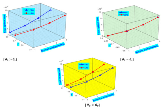
Figure 7. Graphical representation of total cost under a number of shipments.

In Table 7, the following changes are observed:

• If the rate of deterioration of OW is greater than RW, then if the retailer increases the number of shipments, then the total cost increases and the total cost decreases if the retailer decreases the number of shipments, and the policy suggested is FIFO.
• If the degradation rate in OW is equal to the rate in RW and if the retailer increases the number of shipments, then the overall cost will rise significantly. And if the retailer increases the number of shipments, then the total cost decreases more and in this situation, suggests FIFO or LIFO as the appropriate policy.
• If the retailer increases the number of shipments and the rate of degradation of OW is lower than that of RW, in this situation, the overall cost will increase. And suppose the retailer reduces the number of shipments. In that case, the overall cost of the inventory system falls even further, and the suggested policy, in this case, is LIFO, as shown in Figure 7.

Table 8 shows the total optimal cost of the proposed warehouse inventory system for various values of interval-valued parameter $\lambda$ under different deterioration rates. A decision-maker can choose the value of the interval-valued parameter $\lambda$ based on real market conditions. If the retailer increases the value of parameter $\lambda$, the optimal quantity, the optimal replenishment cycle, and the optimal cost decrease both policies. However, the optimal cost decreases up to $\lambda =0.75$, but the value of the total optimal cost increases for the value of $\lambda$ above 0.75, as can be seen in Figure 8. So, for this numerical example, $\lambda =0.75$ gives less optimal cost but choosing $\lambda$ value is the decision-maker’s choice.

Table 8. Optimal cost of inventory system for different interval-valued parameter $\lambda$.

$\mathit{\lambda }$	Deterioration	${\mathit{K}}_{\mathit{F}}^{\ast }$	${\mathit{T}}^{\ast }\left(\mathbf{Year}\right)$	$\mathit{T}\mathit{A}{\mathit{C}}_{\mathit{F}}^{\ast }$	${\mathit{K}}_{\mathit{L}}^{\ast }$	${\mathit{T}}^{\ast }\left(\mathbf{Year}\right)$	$\mathit{T}\mathit{A}{\mathit{C}}_{\mathit{L}}^{\ast }$	Policy Suggested
0	${\theta }_o>{\theta }_r$ ${\theta }_o={\theta }_r$ ${\theta }_o<{\theta }_r$	1487.52 1402.32 925.376	0.748099 0.705743 0.537326	521,374 521,037 521,853	1194.36 1401.10 1128.34	0.650779 0.705353 0.605140	522,121 521,041 521,358	FIFO Either LIFO
0.25	${\theta }_o>{\theta }_r$ ${\theta }_o={\theta }_r$ ${\theta }_o<{\theta }_r$	1419.96 1333.48 885.381	0.742951 0.698246 0.530991	511,191 510,822 511,603	1132.82 1332.41 1089.70	0.640643 0.697877 0.603392	511,935 510,825 511,115	FIFO Either LIFO
0.5	${\theta }_o>{\theta }_r$ ${\theta }_o={\theta }_r$ ${\theta }_o<{\theta }_r$	1347.32 1259.77 846.659	0.736153 0.688915 0.523788	507,257 506,846 507,582	1066.17 1259.77 1047.65	0.628792 0.688915 0.601486	507,992 506,846 507,106	FIFO Either LIFO
0.75	${\theta }_o>{\theta }_r$ ${\theta }_o={\theta }_r$ ${\theta }_o<{\theta }_r$	1269.72 1181.45 800.333	0.727912 0.6779600.515958	512,342 511,876 512,556	996.072 1184.67 1003.14	0.616104 0.679244 0.600098	513,059 511,866 512,095	FIFO Either LIFO
1	${\theta }_o>{\theta }_r$ ${\theta }_o={\theta }_r$ ${\theta }_o<{\theta }_r$	1187.90 1099.57 750.394	0.719202 0.666433 0.508592	530,806 530,263 530,874	926.441 1110.46 958.499	0.605131 0.671070 0.601070	531,490 530,230 530,429	FIFO Either LIFO

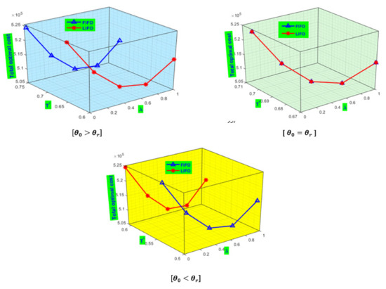
Figure 8. Graphical representation of total cost under various values of $\lambda$.

Sensitivity analysis was carried out by changing one parameter value −20% to 20% and keeping other parameters constant. Under the same holding and deterioration costs of both OW and RW, the total quantity, replenishment cycle, and cost are the same in both FIFO and LIFO policies. The following facts emerged as a result of the parameters’ sensitivity analysis:

• Suppose the selling price ($\tilde{P})$ rises by 20%. The optimal total average cost of the warehouse inventory system decreases moderately due to increasing the selling price, and sales of the product reduce moderately. Consequently, the optimal cycle length increases because the demand for this warehouse inventory system depends on the selling price. Similarly, if the retailer decreases the selling price, then the optimal cost increases and the optimal cycle length decreases (Figure 9).
  

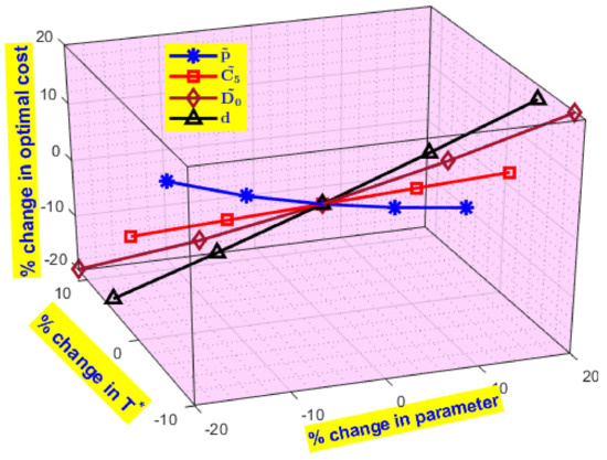  Figure 9. Changes in optimal cost by variations of inventory parameters.
• The presented inventory model is less sensitive to purchasing cost ${\tilde{C}}_5$. It shows that if the purchasing cost of the item increases (decreases), then the total cost increases (decreases) but a very less amount. Increasing or decreasing the purchasing cost shows negligible changes in the replenishment cycle and optimal quantity.
• Suppose transportation distance $d$ increases, then the transportation cost increases so that the optimal cost of the inventory system increases highly. The cycle length and ideal amount are substantially reduced with an increase in the transportation distance. In the same way, the transportation distance $d$ decreases, and then the transportation cost decreases so that the total cost decreases.
• If the tax ($\tilde{\varphi }$) for emitted carbon increases, then the optimal cost of the inventory system increases in lesser quantity, as shown in Figure 10.
  

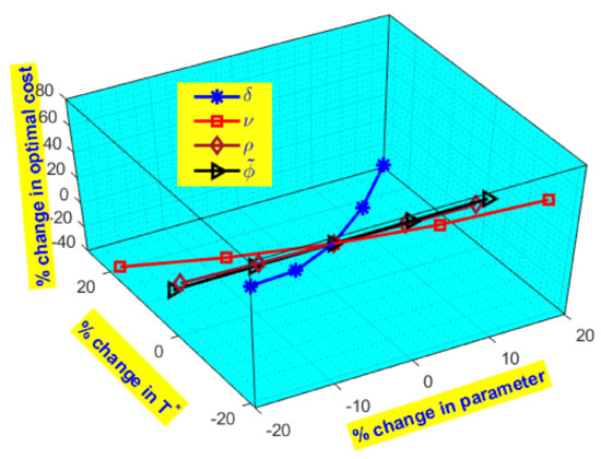  Figure 10. Variations in optimal cost due to changes in system parameters.
• The proposed two-warehouse inventory system’s demand depends on the price-sensitive parameter. From Table 9, we can observe that the optimal total cost is highly sensitive to the price-sensitive parameter $\left(\delta \right)$. This study shows that when a commodity’s price sensitivity rises, demand for the commodity declines rapidly, which lowers order quantities and the inventory system’s optimal total cost while lengthening the replenishment cycle.
  Table 9. Sensitivity analysis of the total inventory cost under the same holding and deterioration costs of both OW and RW.

  Parameter	% Change	${\mathit{K}}_{\mathit{F}}^{\ast }\left(={\mathit{K}}_{\mathit{L}}^{\ast }\right)$	$\% \mathbf{Change} {\mathit{K}}_{\mathit{F}}^{\ast }\left(={\mathit{K}}_{\mathit{L}}^{\ast }\right)$	${\mathit{T}}^{\ast }\left(\mathbf{Year}\right)$	$\% \mathbf{Change} {\mathit{T}}^{\ast }$	$\mathit{T}\mathit{A}{\mathit{C}}_{\mathit{F}}^{\ast }$$(=\mathit{T}\mathit{A}{\mathit{C}}_{\mathit{L}}^{\ast })$	$\% \mathbf{Change} \mathit{T}\mathit{A}{\mathit{C}}_{\mathit{F}}^{\ast }$$(=\mathit{T}\mathit{A}{\mathit{C}}_{\mathit{L}}^{\ast })$
  $\tilde{P}$	−20 −10 10 20	1346.30 1299.90 1224.56 1193.30	6.87 3.19 −2.79 −5.28	0.645072 0.667866 0.708509 0.726866	−6.36 −3.06 2.84 5.51	578,102 539,307 479,193 455,288	14.06 6.40 −5.46 −10.17
  ${\tilde{C}}_5$	−20 −10 10 20	1270.63 1265.17 1254.43 1249.14	0.86 0.43 −0.42 −0.84	0.692906 0.690899 0.686953 0.685014	0.60 0.29 −0.28 −0.57	495,735 501,290 512,401 517,957	−2.19 −1.00 1.10 2.19
  $d$	−20 −10 10 20	1348.69 1302.22 1220.80 11184.85	7.06 3.37 −3.09 −5.95	0.720896 0.704096 0.675125 0.662541	4.64 2.20 −2.00 −3.82	417,420 462,136 551,550 596,249	−17.64 −8.82 8.82 17.64
  $\tilde{\varphi }$	−20 −10 10 20	1267.56 1263.65 1255.94 1252.15	0.62 0.31 −0.30 −0.60	0.691181 0.690039 0.687808 0.686718	0.33 0.16 −0.16 −0.32	499,079 502,963 510,729 514,612	−1.53 −0.77 0.77 1.53
  $\delta$	−20 −10 10 20	1606.80 1422.57 1115.95 988.955	27.55 12.92 −11.42 −21.50	0.541359 0.610811 0.776645 0.875043	−21.42 −11.34 12.73 27.02	820,890 644,791 398,780 314,115	61.96 27.22 −21.32 −38.03
  $\rho$	−20 −10 10 20	1210.61 1234.30 1287.26 1317.055	−3.90 −2.02 2.18 4.55	0.675093 0.681648 0.696995 0.706007	−2.01 −1.05 1.17 2.48	560,142 533,496 480,193 453,537	10.52 5.26 −5.26 −10.52
  $\nu$	−20 −10 10 20	1079.00 1165.80 1361.50 1471.59	−14.35 −7.46 8.08 18.90	0.802917 0.743816 0.637946 0.590650	16.55 7.97 −7.40 −14.26	373,103 434,769 591,094 689,572	−26.39 −14.22 16.62 36.05
  $a$	−20 −10 10 20	1057.91 1158.34 1360.89 1460.35	−16.02 −8.05 8.03 15.92	0.615433 0.651613 0.726790 0.764641	−10.67 −5.41 5.50 11.00	507,542 507,180 506,542 506,268	0.12 0.07 −0.06 −0.11
  $b$	−20 −10 10 20	1255.75 1257.95 1261.27 1262.50	−0.32 −0.14 0.12 0.22	0.687752 0.688389 0.689348 0.689705	−0.17 −0.08 0.06 0.11	510,927 508,683 505,342 504,110	0.8 0.36 −0.30 −0.54
  $D_o$	−20 −10 10 20	1126.17 1194.83 1321.54 1380.55	−18.90 −9.45 9.45 18.89	0.769678 0.725941 0.657041 0.629224	11.72 5.37 −4.63 −8.67	406,034 456,449 557,228 607,598	−19.89 −9.94 9.9419.88

• The amount of carbon emission due to green technology ($\rho$) increases, then the total cost of the inventory system decreases moderately but cycle length and optimal quantity increase, but the increasing rate is less. If the impact of advertisement ($\nu$) increases, then the sales of the product increase so that the total inventory cost and optimal quantity increase is high, but the cycle length decreases due to the rise in sales of the product as well as emptying the warehouse quickly as shown in Figure 10.
• If controlling parameter of preservation technology ($a$) in both OW and RW increases, then the cycle length and optimal quantity increase greatly because under controlling parameter, the deterioration reduces so that the cycle length and quantity increase greatly and total cost decreases.
• If the efficiency of greener technology (b) increases, then the total cost decreases but optimal cycle length and quantity increase.
• If the product’s initial demand $D_o$ increases, then the optimal total cost of the warehouse inventory system increases and optimal quantity also increases, but the replenishment cycle length decreases moderately. Since sales have increased, the inventory has been holding less time in the warehouses, so cycle length decreases automatically. If the demand decreases, then the sales of the product reduce so that automatically total cost and quantity reduce greatly, but the cycle length increases moderately due to less demand; the product stays for a prolonged period in the warehouses so that the total cycle length increases gradually.

Managerial Implications

The implications of this study is generally for the proposed two-warehouse inventory management where the following scenarios will happen: (i) The deterioration of RW is less than the OW due to extra facilities of RW; (ii) sometimes the deterioration of OW is less than the RW; (iii) in general, the holding cost of OW is less than the RW; (iv) due to the competition of warehouse marketing, the holding cost of RW is less than or equal to the OW rarely; and (v) the items in RW are stored only after entirely utilizing the capacity of OW. All these managerial concepts are validated in this study.

This model explains all these scenarios and suggests a suitable dispatch policy for the two-warehouse inventory management systems. This study was developed by taking the capacity of OW as fixed, but in reality, retailer shows interest in storing items in RW due to the high facilities of RW even though the unlimited capacity of OW. So, this concept can expend by considering the unlimited storage capacity of OW.

The green warehouse model may help in making decisions to advance the sustainable warehouse inventory system by optimizing cycle time and order quantity. Incorporating carbon emission costs into the model will also help firms concentrate on reducing the warehouse’s overall inventory. That will lower the cost of storing products while reducing carbon emissions. As the vehicle’s fuel usage rises, the overall cost also grows, which is another concern. The entire cost of the inventory system concurrently reduces as the efficiency of green technology (b) increases. Lower inventory’s total cost is the result of higher efficiency.

Proper utilization of warehouse inventory systems plays a significant role in business management. This study can apply to storing highly deteriorated items such as vegetables, milk, fruits, etc. The implementation of the proposed green warehouse inventory management is an eco-friendly concept. Recently, many companies have shown interest in making their warehouses green to make this study more beneficial.

7. Conclusions

This paper presented price-sensitive demand, i.e., if the item has a high price, then the majority of the customers are not interested in buying it. As a result, the demand for that commodity will fall and directly impact the inventory management system for such a decline in order (Table 9). In recent trends, the need for herbal products has increased because herbal or natural products are made using natural resources. Furthermore, herbal or natural products do not have harmful chemicals, so they do not have any side effects. Many people are conscious about their health, so if the product contains herbal or natural ingredients, the product demand increases; at the same time, if the product contains chemical ingredients, then the demand decreases. Mainly, this study may be much more appropriate for such order of skin care, hair care, body care, and food ingredients commodities (Table 6).

Advertising plays an important role in the awareness of today’s society. Most of the product’s demand depends on the impact of the promotion. This study described the effects of advertising if the product’s info reaches the customer quickly, then the sales of the product increase, i.e., the demand rate increases (Figure 10). In two-warehousing inventory systems, deterioration of the item is a common phenomenon that the stock of the inventory system spoils. This study revealed the impact of additional preservation facilities on both OW and RW in order to overcome such a circumstance. Holding cost plays the most crucial role in two-warehousing systems. Generally, the holding cost of RW is greater than the OW, but this study has shown the competition in the warehouse market by considering the holding cost of RW is less than or equal to OW, and then considering all those circumstances attempted to suggest suitable dispatch policy as shown in Table 5.

The space of warehouses of large operational companies may vary for different items because of the need to arrange various things in different shapes of shelves. Here this model considered the composition of the storage capacity of OW to be a triangular Pythagorean fuzzy shape. However, this model is also useful for the other fuzzy capacities of owned warehouses. Recently, most businesses are governed to operate in a green environment to avoid pollution in warehouses, production units, shopping malls, marketplaces, etc. This warehouse inventory system was developed based on a sustainable environment under a carbon tax policy. This study considered emissions released from transporting, holding, and deteriorating items in OW and RW. The effect of the use of green technology to keep the environment less polluted has been discussed. This research interlined the investment in green technology even though the optimal cost is reduced (Table 4).

By altering one parameter while keeping the others constant, this model performed sensitivity analyses for both FIFO and LIFO strategies. Under sensitivity, the results show that a higher carbon tax benefits the environment along with green technology (Figure 10). The two-warehouse inventory systems may be expanded in a number of ways for future studies by incorporating the variable capacity of OW and RW. For further study, one can consider the related inventory costs, preservation, and green parameters as interval or fuzzy numbers. Additionally, the demand may be shown as a function of the price, advertising, and other factors, with the coefficients represented as interval numbers.

There are certain limitations to the proposed sustainable model. This model considers the carbon emission cost under a simple carbon-tax policy. At the same time, some models ([56,59]) computed carbon tax using a cap and trade, cap and reward, and strictly permitted cap policies. Hence, future research may develop two-warehouse models under various carbon tax policies. This model combinedly invested green technology investment in OW and RW. So, this model can further develop by individually investing in green technology investment to OW and RW.

References

- Ishii, H.; Nose, T. Perishable inventory control with two types of customers and different selling prices under the warehouse capacity constraint. Int. J. Prod. Econ. 1996, 44, 167–176. [Google Scholar] [CrossRef]
- Dye, C.Y.; Ouyang, L.Y.; Hsieh, T.P. Deterministic inventory model for deteriorating items with capacity constraint and time proportional backlogging rate. Eur. J. Oper. Res. 2007, 178, 789–807. [Google Scholar] [CrossRef]
- Das, B.; Maity, K.; Maiti, M. A Two Warehouse Supply-Chain Model under Possibility/Necessity/Credibility Measures. Math. Comput. Model. 2007, 46, 398–409. [Google Scholar] [CrossRef]
- Liang, Y.; Zhou, F. A two-warehouse inventory model for deteriorating items under conditionally permissible delay in payment. Appl. Math. Model. 2011, 35, 2221–2231. [Google Scholar] [CrossRef]
- Bhunia, A.K.; Jaggi, C.K.; Sharma, A.; Sharma, R. A two-warehouse inventory model for deteriorating items under permissible delay in payment with partial backlogging. Appl. Math. Comput. 2014, 232, 1125–1137. [Google Scholar] [CrossRef]
- Pasandideh, S.H.R.; Niaki, S.T.A.; Nobil, A.H.; Cárdenas-Barrón, L.E. A multi product single machine economic production quantity model for an imperfect production system under warehouse construction cost. Int. J. Prod. Econ. 2015, 169, 203–214. [Google Scholar] [CrossRef]
- Zhou, J.R.; Zhang, H.J.; Zhou, H.L. Localization of pallets in warehouses using passive RFID system. J. Cent. South Univ. 2015, 22, 3017–3025. [Google Scholar] [CrossRef]
- Chakraborty, D.; Jana, D.K.; Roy, T.K. Two-warehouse partial backlogging inventory model with ramp type demand rate, three-parameter Weibull distribution deterioration under inflation and permissible delay in payments. Comput. Ind. Eng. 2018, 123, 157–179. [Google Scholar] [CrossRef]
- Jaggi, C.K.; Verma, P.; Gupta, M. Ordering policy for non-instantaneous deteriorating items in two warehouse environment with shortages. Int. J. Logist. Syst. Manag. 2015, 22, 103–124. [Google Scholar] [CrossRef]
- Tsao, Y.C. Designing a supply chain network for deteriorating inventory under preservation effort and trade credits. Int. J. Prod. Res. 2016, 54, 3837–3851. [Google Scholar] [CrossRef]
- Giri, B.; Pal, H.; Maiti, T. A vendor-buyer supply chain model for time-dependent deteriorating item with preservation technology investment. Int. J. Math. Oper. Res. 2017, 10, 431–449. [Google Scholar] [CrossRef]
- Rong, M.; Mahapatra, N.K.; Maiti, M. A two warehouse inventory model for a deteriorating item with partially/fully backlogged shortage and fuzzy lead time. Eur. J. Oper. Res. 2008, 189, 59–75. [Google Scholar] [CrossRef]
- Lee, C.C.; Hsu, S.L. A two-warehouse production model for deteriorating inventory items with time-dependent demands. Eur. J. Oper. Res. 2009, 194, 700–710. [Google Scholar] [CrossRef]
- Bhavani, G.D.; Georgise, F.B.; Mahapatra, G.; Maneckshaw, B. Neutrosophic Cost Pattern of Inventory System with Novel Demand Incorporating Deterioration and Discount on Defective Items Using Particle Swarm Algorithm. Comput. Intell. Neurosci. 2022, 2022, 7683417. [Google Scholar] [CrossRef]
- Govindan, K.; Khodaverdi, R.; Vafadarnikjoo, A. Intuitionistic fuzzy based DEMATEL method for developing green practices and performances in a green supply chain. Expert Syst. Appl. 2015, 42, 7207–7220. [Google Scholar] [CrossRef]
- Mahapatra, G.S.; Adak, S.; Kaladhar, K. A fuzzy inventory model with three parameter Weibull deterioration with reliant holding cost and demand incorporating reliability. J. Intell. Fuzzy Syst. 2019, 36, 5731–5744. [Google Scholar] [CrossRef]
- Wu, K.S.; Ouyang, L.Y.; Yang, C.T. An optimal replenishment policy for non-instantaneous deteriorating items with stock dependent demand and partial backlogging. Int. J. Prod. Econ. 2006, 101, 369–384. [Google Scholar] [CrossRef]
- Das, S.K.; Pervin, M.; Roy, S.K.; Weber, G.W. Multi-objective solid transportation-location problem with variable carbon emission in inventory management: A hybrid approach. Ann. Oper. Res. 2021. [Google Scholar] [CrossRef]
- Taleizadeh, A.A.; Hazarkhani, B.; Moon, I. Joint pricing and inventory decisions with carbon emission considerations, partial backordering and planned discounts. Ann. Oper. Res. 2020, 290, 95–113. [Google Scholar] [CrossRef]
- Murmu, V.; Kumar, D.; Sarkar, B.; Mor, R.S.; Jha, A.K. Sustainable inventory management based on environmental policies for the perishable products under first or last in and first out policy. J. Ind. Manag. Optim. 2022. [Google Scholar] [CrossRef]
- Milewska, B.; Milewski, D. Implications of Increasing Fuel Costs for Supply Chain Strategy. Energies 2022, 15, 6934. [Google Scholar] [CrossRef]
- Jaggi, C.; Tiwari, S.; Shafi, A. Effect of deterioration on two-warehouse inventory model with imperfect quality. Comput. Ind. Eng. 2015, 88, 378–385. [Google Scholar] [CrossRef]
- Sanni, S.; Chukwu, W. An Economic order quantity model for Items with Three-parameter Weibull distribution Deterioration, Ramp-type Demand and Shortages. Appl. Math. Model. 2013, 37, 9698–9706. [Google Scholar] [CrossRef]
- Kumar, A.; Chanda, U. Two-warehouse inventory model for deteriorating items with demand influenced by innovation criterion in growing technology market. J. Manag. Anal. 2018, 5, 198–212. [Google Scholar] [CrossRef]
- Jaggi, C.K.; Verma, P. A deterministic order level inventory model for deteriorating items with two storage facilities under FIFO dispatching policy. Int. J. Procure. Manag. 2010, 3, 265–278. [Google Scholar] [CrossRef]
- Ouyang, L.Y.; Ho, C.H.; Su, C.H.; Yang, C.T. An integrated inventory model with capacity constraint and order-size dependent trade credit. Comput. Ind. Eng. 2015, 84, 133–143. [Google Scholar] [CrossRef]
- Howard, C.; Marklund, J.; Tan, T.; Reijnen, I. Inventory control in a spare parts distribution system with emergency stocks and pipeline information. Manuf. Serv. Oper. Manag. 2015, 17, 142–156. [Google Scholar] [CrossRef]
- Gong, F.; Wei, Z. Warehouse goods inventory optimization based on the improved adaptive genetic algorithm. J. Comput. Inf. Syst. 2015, 11, 5293–5306. [Google Scholar] [CrossRef]
- Budiawan, R.; Simanjuntak, J.; Rosely, E. Inventory management application of drug using FIFO method. Test Eng. Manag. 2020, 83, 7785–7791. [Google Scholar]
- Shu, J.; Wu, T.; Zhang, K. Warehouse location and two-echelon inventory management with concave operating cost. Int. J. Prod. Res. 2015, 53, 2718–2729. [Google Scholar] [CrossRef]
- Diabat, A.; Theodorou, E. A location-inventory supply chain problem: Reformulation and piecewise linearization. Comput. Ind. Eng. 2015, 90, 381–389. [Google Scholar] [CrossRef]
- Huang, H.; He, Y.; Li, D. Pricing and inventory decisions in the food supply chain with production disruption and controllable deterioration. J. Clean. Prod. 2018, 180, 280–296. [Google Scholar] [CrossRef]
- Yang, C.T.; Dye, C.Y.; Ding, J.F. Optimal dynamic trade credit and preservation technology allocation for a deteriorating inventory model. Comput. Ind. Eng. 2015, 87, 356–369. [Google Scholar] [CrossRef]
- Yadav, D.; Kumari, R.; Kumar, N.; Sarkar, B. Reduction of waste and carbon emission through the selection of items with cross-price elasticity of demand to form a sustainable supply chain with preservation technology. J. Clean. Prod. 2021, 297, 126298. [Google Scholar] [CrossRef]
- Sepehri, A.; Mishra, U.; Sarkar, B. A sustainable production-inventory model with imperfect quality under preservation technology and quality improvement investment. J. Clean. Prod. 2021, 310, 127332. [Google Scholar] [CrossRef]
- Mishra, U.; Wu, J.Z.; Tsao, Y.C.; Tseng, M.L. Sustainable inventory system with controllable non-instantaneous deterioration and environmental emission rates. J. Clean. Prod. 2020, 244, 118807. [Google Scholar] [CrossRef]
- Jaggi, C.K.; Khanna, A.; Verma, P. Two-warehouse partial backlogging inventory model for deteriorating items with linear trend in demand under inflationary conditions. Int. J. Syst. Sci. 2011, 42, 1185–1196. [Google Scholar] [CrossRef]
- Singh, T.; Pattnayak, H. A two-warehouse inventory model for deteriorating items with linear demand under conditionally permissible delay in payment. Int. J. Manag. Sci. Eng. Manag. 2014, 9, 104–113. [Google Scholar] [CrossRef]
- Lee, Y.P.; Dye, C.Y. An inventory model for deteriorating items under stock-dependent demand and controllable deterioration rate. Comput. Ind. Eng. 2012, 63, 474–482. [Google Scholar] [CrossRef]
- Jaggi, C.K.; Pareek, S.; Verma, P.; Sharma, R. Ordering policy for deteriorating items in a two-warehouse environment with partial backlogging. Int. J. Logist. Syst. Manag. 2013, 16, 16–40. [Google Scholar] [CrossRef]
- Shastri, A.; Singh, S.; Yadav, D.; Gupta, S. Supply chain management for two-level trade credit financing with selling price dependent demand under the effect of preservation technology. Int. J. Procure. Manag. 2014, 7, 695–718. [Google Scholar] [CrossRef]
- Sanni, S.S.; Chukwu, W.I.E. An Inventory Model with Three-Parameter Weibull Deterioration, Quadratic Demand Rate and Shortages. Am. J. Math. Manag. Sci. 2016, 35, 159–170. [Google Scholar] [CrossRef]
- Jaggi, C.K.; Goel, S.K.; Tiwari, S. Two-warehouse inventory model for non-instantaneous deteriorating items under different dispatch policies. Investig. Oper. 2017, 38, 343–365. [Google Scholar]
- Dye, C.Y.; Yang, C.T.; Wu, C.C. Joint dynamic pricing and preservation technology investment for an integrated supply chain with reference price effects. J. Oper. Res. Soc. 2018, 69, 811–824. [Google Scholar] [CrossRef]
- Shaikh, A.; Cárdenas-Barrón, L.; Tiwari, S. A two-warehouse inventory model for non-instantaneous deteriorating items with interval-valued inventory costs and stock-dependent demand under inflationary conditions. Neural Comput. Appl. 2019, 31, 1931–1948. [Google Scholar] [CrossRef]
- Xu, C.; Zhao, D.; Min, J.; Hao, J. An inventory model for nonperishable items with warehouse mode selection and partial backlogging under trapezoidal-type demand. J. Oper. Res. Soc. 2021, 72, 744–763. [Google Scholar] [CrossRef]
- Sarkar, B.; Dey, B.K.; Sarkar, M.; Kim, S.J. A smart production system with an autonomation technology and dual channel retailing. Comput. Ind. Eng. 2022, 173, 108607. [Google Scholar] [CrossRef]
- Maiti, M.K.; Maiti, M. Fuzzy inventory model with two warehouses under possibility constraints. Fuzzy Sets Syst. 2006, 157, 52–73. [Google Scholar] [CrossRef]
- Panda, D.; Maiti, M.K.; Maiti, M. Two warehouse inventory models for single vendor multiple retailers with price and stock dependent demand. Appl. Math. Model. 2010, 34, 3571–3585. [Google Scholar] [CrossRef]
- Guchhait, P.; Maiti, M.K.; Maiti, M. Two storage inventory model of a deteriorating item with variable demand under partial credit period. Appl. Soft Comput. 2013, 13, 428–448. [Google Scholar] [CrossRef]
- Shabani, S.; Mirzazadeh, A.; Sharifi, E. A two-warehouse inventory model with fuzzy deterioration rate and fuzzy demand rate under conditionally permissible delay in payment. J. Ind. Prod. Eng. 2016, 33, 134–142. [Google Scholar] [CrossRef]
- Wang, H.; Zhang, F.; Ullah, K. Waste Clothing Recycling Channel Selection Using a CoCoSo-D Method Based on Sine Trigonometric Interaction Operational Laws with Pythagorean Fuzzy Information. Energies 2022, 15, 2010. [Google Scholar] [CrossRef]
- Dorfeshan, Y.; Allah Taleizadeh, A.; Toloo, M. Assessment of risk-sharing ratio with considering budget constraint and disruption risk under a triangular Pythagorean fuzzy environment in public–private partnership projects. Expert Syst. Appl. 2022, 203, 117245. [Google Scholar] [CrossRef]
- Paul, A.; Pervin, M.; Roy, S.K.; Maculan, N.; Weber, G.W. A green inventory model with the effect of carbon taxation. Ann. Oper. Res. 2022, 309, 233–248. [Google Scholar] [CrossRef]
- Pan, J.L.; Chiu, C.Y.; Wu, K.S.; Yang, C.T.; Wang, Y.W. Optimal Pricing, Advertising, Production, Inventory and Investing Policies in a Multi-Stage Sustainable Supply Chain. Energies 2021, 14, 7544. [Google Scholar] [CrossRef]
- Sarkar, B.; Kar, S.; Basu, K.; Guchhait, R. A sustainable managerial decision-making problem for a substitutable product in a dual-channel under carbon tax policy. Comput. Ind. Eng. 2022, 172, 108635. [Google Scholar] [CrossRef]
- Daryanto, Y.; Wee, H.M.; Wu, K.H. Revisiting sustainable EOQ model considering carbon emission. Int. J. Manuf. Technol. Manag. 2021, 35, 1–11. [Google Scholar] [CrossRef]
- Li, Z.; Hai, J. Inventory management for one warehouse multi-retailer systems with carbon emission costs. Comput. Ind. Eng. 2019, 130, 565–574. [Google Scholar] [CrossRef]
- Che, C.; Zheng, H.; Geng, X.; Chen, Y.; Zhang, X. Research on Carbon Emission Reduction Investment Decision of Power Energy Supply Chain—Based on the Analysis of Carbon Trading and Carbon Subsidy Policies. Energies 2022, 15, 6151. [Google Scholar] [CrossRef]
- Shen, L.; Olfat, L.; Govindan, K.; Khodaverdi, R.; Diabat, A. A fuzzy multi criteria approach for evaluating green supplier’s performance in green supply chain with linguistic preferences. Resour. Conserv. Recycl. 2013, 74, 170–179. [Google Scholar] [CrossRef]
- Jaggi, C.K.; Pareek, S.; Khanna, A.; Sharma, R. Credit financing in a two-warehouse environment for deteriorating items with price-sensitive demand and fully backlogged shortages. Appl. Math. Model. 2014, 38, 5315–5333. [Google Scholar] [CrossRef]
- Cheng, C.; Qi, M.; Wang, X.; Zhang, Y. Multi-period inventory routing problem under carbon emission regulations. Int. J. Prod. Econ. 2016, 182, 263–275. [Google Scholar] [CrossRef]
- Xu, X.; Bai, Q.; Chen, M. A comparison of different dispatching policies in two-warehouse inventory systems for deteriorating items over a finite time horizon. Appl. Math. Model. 2017, 41, 359–374. [Google Scholar] [CrossRef]
- Huang, Y.S.; Fang, C.C.; Lin, Y.A. Inventory management in supply chains with consideration of Logistics, green investment and different carbon emissions policies. Comput. Ind. Eng. 2020, 139, 106207. [Google Scholar] [CrossRef]
- San-José, L.A.; Sicilia, J.; Abdul-Jalbar, B. Optimal policy for an inventory system with demand dependent on price, time and frequency of advertisement. Comput. Oper. Res. 2021, 128, 105169. [Google Scholar] [CrossRef]
- Rana, R.; Kumar, D.; Prasad, K. Two warehouse dispatching policies for perishable items with freshness efforts, inflationary conditions and partial backlogging. Oper. Manag. Res. 2021, 15, 28–45. [Google Scholar] [CrossRef]
- Khara, B.; Dey, J.; Mondal, S. An integrated imperfect production system with advertisement dependent demand using branch and bound technique. Flex. Serv. Manuf. J. 2021, 33, 508–546. [Google Scholar] [CrossRef]
- Hasan, M.R.; Roy, T.C.; Daryanto, Y.; Wee, H.M. Optimizing inventory level and technology investment under a carbon tax, cap-and-trade and strict carbon limit regulations. Sustain. Prod. Consum. 2021, 25, 604–621. [Google Scholar] [CrossRef]
- Ruidas, S.; Seikh, M.R.; Nayak, P.K. A production inventory model with interval-valued carbon emission parameters under price-sensitive demand. Comput. Ind. Eng. 2021, 154, 107154. [Google Scholar] [CrossRef]
- Bhavani, G.D.; Meidute-Kavaliauskiene, I.; Mahapatra, G.S.; Činčikaitė, R. A Sustainable Green Inventory System with Novel Eco-Friendly Demand Incorporating Partial Backlogging under Fuzziness. Sustainability 2022, 14, 9155. [Google Scholar] [CrossRef]
- Yager, R.R. Pythagorean Membership Grades in Multicriteria Decision Making. IEEE Trans. Fuzzy Syst. 2014, 22, 958–965. [Google Scholar] [CrossRef]
- Umer, R.; Touqeer, M.; Omar, A.; Ahmadian, A.; Salahshour, S.; Ferrara, M. Selection of solar tracking system using extended TOPSIS technique with interval type-2 pythagorean fuzzy numbers. Optim. Eng. 2021, 22, 2205–2231. [Google Scholar] [CrossRef]
- Roubens, M. Inequality Constraints between Fuzzy Numbers and Their Use in Mathematical Programming. In Stochastic versus Fuzzy Approaches to Multiobjective Mathematical Programming under Uncertainty; Springer: Dordrecht, The Netherlands, 1990; pp. 321–330. [Google Scholar] [CrossRef]
- Mahapatra, G.S.; Mandal, T.K. Posynomial Parametric Geometric Programming with Interval Valued Coefficient. J. Optim. Theory Appl. 2012, 154, 120–132. [Google Scholar] [CrossRef]
- Cambini, A.; Martein, L. Generalized Convexity and Optimization: Theory and Applications; Springer: Berlin/Heidelberg, Germany, 2009. [Google Scholar]
Publisher’s Note: MDPI stays neutral with regard to jurisdictional claims in published maps and institutional affiliations. |
© 2022 by the authors. Licensee MDPI, Basel, Switzerland. This article is an open access article distributed under the terms and conditions of the Creative Commons Attribution (CC BY) license (https://creativecommons.org/licenses/by/4.0/).