Recurrent Neural Network-Based Nonlinear Optimization for Braking Control of Electric Vehicles

Abstract

In this paper, electro-hydraulic braking (EHB) force allocation for electric vehicles (EVs) is modeled as a constrained nonlinear optimization problem (NOP). Recurrent neural networks (RNNs) are advantageous in many folds for solving NOPs, yet existing RNNs’ convergence usually requires convexity with calculation of second-order partial derivatives. In this paper, a recurrent neural network-based NOP solver (RNN-NOPS) is developed. It is seen that the RNN-NOPS is designed to drive all state variables to asymptotically converge to the feasible region, with loose requirement on the NOP’s first-order partial derivative. In addition, the RNN-NOPS’s equilibria are proved to meet Karush–Kuhn–Tucker (KKT) conditions, and the RNN-NOPS behaves with a strong robustness against the violation of the constraints. The comparative studies are conducted to show RNN-NOPS’s advantages for solving the EHB force allocation problem, it is reported that the overall regenerative energy of RNN-NOPS is 15.39% more than that of the method for comparison under SC03 cycle.

1. Introduction

The momentum of the development of pure electric vehicles (EVs) has been increasing due to the shortage of foreseeable fossil fuel and the air pollution caused from fossil fuel combustion. Limited battery power, however, has become one of the main shortcomings influencing EVs’ further commercialization. Recently, many efficient energy management strategies have been developed, offering a significant improvement of EV’s performance. It has been shown that in urban driving, the energy consumed in braking is almost half of the total traction power [1]. Therefore, an effective electro-hydraulic braking (EHB) force allocation strategy is required for achieving optimal regenerative energy while guaranteeing the braking safety.

Various optimization and control algorithms have been developed for regenerative braking control. In [2], given the desired yaw moment and road friction coefficient, the regenerative and EHB torque can be designed by using a genetic algorithm (GA). It is noted that the quality of a GA’s solution could be improved by using a larger initial population, which, however, would increase GA’s computational cost; GA also suffers from premature convergence [3]. A regenerative braking control method based on model predictive control (MPC) was proposed in [4], where maximization of energy recuperation and wheel slip regulation are achieved. However, it has been noted that high-quality system models built with accurate measurement data are required by MPC, which may increase model complexity and computational cost [5].

To attain optimal recovered energy with braking safety guaranteed, the EHB force allocation problem of EVs has been treated as a nonlinear optimization problem (NOP) recently. The NOP is widely used in portfolio optimization [6,7,8], system control [9,10,11,12], and machine learning [13]. For solving NOPs, many numerical algorithms have been proposed over decades [14,15]. It has been noted that the NOP algorithms’ computing cost is highly affected by the dimension of the state variable vector and the complexity of the NOP solvers’ structures and thus, most of these algorithms are less effective in real-time applications as pointed out in [16,17].

Since Tank and Hopfield’s work [18], many recurrent neural networks (RNNs) have been available for solving NOPs. The benefits of the RNN-based methods are threefold: (i) the availability of electronic implementation by using very large-scale integration (VLSI) chips, (ii) the capability of solving NOPs with time-varying parameters, (iii) the efficiency of applying the numerical ordinary differential equation (ODE) techniques for solving NOPs [17]. Variants of RNN such as long short-term memory (LSTM) have been employed for battery state of health and power consumption forecasting [19]. Since the proposal of neural differential equations [20], where Residual NN [21] was proposed to be a discretized ODE. It has been a trend to bridge neural networks and ODEs and exploit off-the-shelf researches on ODEs for further enhancing deep learning strategies. Other neural network-based algorithms, such as an SGTM neural-like structure can also be used to process large amounts of data from a variety of industries [22].

In [16], an RNN was proposed for solving NOPs and it was proved that the state variables can all converge to an exact Karush–Kuhn–Tucker (KKT) point with an assumption on the convexity of both the objective function and constraints. Moreover, a single-layered RNN was developed for solving NOPs in [23], where it is required that the gradients of all inequality constraints equal to 0 and are linearly independent, and other conditions are also necessary for exact penalty. In [24], a neurodynamic model based on an augmented Lagrangian function was proposed; the states of the model are asymptotically stable at a strict local minimum given that the second-order sufficiency conditions (SOSC) [25] holds. In addition to the above typical RNNs, two projection neural networks with reduced model complexity (RDPNNs) for solving NOPs were proposed in [26], where RDPNNs were proved to be globally convergent to the points satisfying the reduced optimality condition, under the condition that the Hessian matrix of the associated Lagrangian function is positive definite at each KKT point.

In this paper, a novel RNN-based NOP solver (RNN-NOPS) is proposed for solving the EHB force allocation of EVs. It will be shown that an RNN-NOPS is not only able to solve NOPs with constraints fully met and optimality guaranteed, but also suitable for a wide category of timely industrial applications. The distinctive contributions of this paper are summarized as follows:

• It is proved that, given the constraint violated, the only equilibrium at the origin of the constraint mapping space ${\mathfrak{R}}^m$ is globally asymptotically stable in the Lyapunov sense, ensuring that all the RNN-NOPS’s state variables are able to reach the feasible region from the outside. This property only requires a first-order partial derivative of the NOP, whose verification costs less computation compared to existing methods.
• The RNN-NOPS’s equilibria are designed to hold the KKT condition and, therefore, the valid local minima of the NOP can be obtained.
• The comparative studies in the simulation section show the advantages of the RNN-NOPS for solving the problem under different braking processes with guaranteed constraints and optimality, compared with the existing optimization-solving approaches discussed in [16].
• The RNN-NOPS is based on the neural network model with parallel structure, which is competent for industrial applications where real-time solutions are required. RNN-NOPS is not only able to solve NOPs with constraints fully met and optimality guaranteed, but also suitable for a wide category of timely industrial applications.

The remainder of this paper is organized as follows. In Section 2, the background of RNN-based optimization approaches and the EHB force allocation problem are briefly introduced. In Section 3, the mechanism and theoretical properties of the RNN-NOPS are discussed in detail. The results of algorithmic comparative studies on EHB force allocation problem are presented in Section 4, followed by the conclusion given in Section 5.

2. Background and Problem Formulation

2.1. RNN-Based Optimization

Consider the following nonlinear optimization problem (NOP) [17]:

$$\begin{array}{l}\min f(x)\\ s.t. c_j(x)\le 0, j=1, ..., m\\ x_i\ge 0, i=1, ..., n\end{array}$$

(1)

where $x={[x_1, ..., x_n]}^T$ is the decision variable vector, $f:R^n\to R$, $c_j:R^n\to R$, $f$ and all $c_j$ are assumed to be twice differentiable.

Given the Lagrangian function of the NOP of the form:

$$L(x, y)=f(x)+{\displaystyle \sum _{j=1}^m{y}_j{c}_j(x)}$$

(2)

where $y={[y_1, ..., y_j, ..., y_m]}^T$ is the Lagrangian multiplier vector. If $x^{*}$ is a local optimal point, then there exists $y^{*}\in R^m$ such that $(x^{*}, y^{*})$ is a Karush–Kuhn–Tucker (KKT) point satisfying [22,27].

$$\left\{\begin{array}{l}\nabla f(x^{*})+{\displaystyle \sum _{j=1}^m\nabla c_j(x^{*})y_j^{*}}=0\\ c_j(x^{*})y_j^{*}=0\\ c_j(x^{*})\le 0\\ y_j^{*}\ge 0, x_i^{*}\ge 0\end{array}\right.$$

(3)

where $\nabla c_j(x^{*})$ and $\nabla f(x^{*})$ are the gradients of the functions $c_j(x)$ and $f(x)$ at $x=x^{*}$, $y=y^{*}$.

Definition 1.

Let $x^{*}$satisfy all the constraints in Equation (1) and $J(x^{*})$is a set of index $j$with $c_j(x^{*})=0$. If the gradients $\nabla c_j(x^{*})$with $j\in J(x^{*})$are linearly independent, then $x^{*}$is called regular point [28].

Lemma 1.

Consider the NOP in Equation (1) with the Lagrangian function in Equation (2). Suppose that $x^{*}$is a regular point of the NOP in Equation (1), $x^{*}$is a strict local minimum of the NOP if (i) there exists $y^{*}$such that $(x^{*}, y^{*})$satisfies KKT conditions in Equation (3); (ii) for any $d\ne 0, d\in {\mathfrak{R}}^n$such that$\nabla c_j{(x^{*})}^{T}d=0$for every $j\in J(x^{*})$, it follows that [28]:

$$d^T[{\nabla }^{2}f(x^{*})+{\displaystyle \sum _j{y}_j^{*}{\nabla }^2{c}_j(x^{*})}]d>0$$

(4)

(iii)$y^{*}$satisfies the strict complementary assumption given by:

$$y_j^{*}>0, \forall j\in J(x^{*})$$

(5)

The conditions (i), (ii) and (iii) in Lemma 1 are called second-order sufficient conditions (SOSC).

In [28], the following augmented Lagrangian function is defined:

$$L_c(x, y)=f(x)+{\displaystyle \sum _{j=1}^m{y}_j^2{c}_j(x)}+\frac{c}{2}{\displaystyle \sum _{j=1}^m{(y_j{c}_j(x))}^2}$$

(6)

where $c$ is a positive penalty parameter. A Lagrange-type neural network is then constructed as:

$$\frac{d{x}_i}{dt}=-{\nabla }_{x_i}{L}_c(x, y), i=1, ..., n$$

(7a)

$$\frac{d{y}_j}{dt}=2y_j{c}_j(x), j=1, ..., m$$

(7b)

It is easy to show that, under SOSC, $(x^{*}, y^{*})$ is a strict local minimum of the augmented Lagrangian function. Furthermore, the neural network modeled in Equation (7a,b) is locally asymptotically stable at its local minimum.

Remark 1.

The discussions in Equations (6) and (7b) describe a generalized framework for designing RNNs. It should be addressed that the augmented Lagrangian function determines both the dynamics of KKT pairs and the stability of the RNN in Equation (7a,b) in a Lyapunov sense. By reasonably constructing the penalty function or the regulating rule, the KKT points could correspond to the largest invariant set in LaSalle’s invariance principle [28,29] and the dynamics of the designed RNN are able to globally converge to the KKT pairs.

Further in [17], an RNN for solving NOP was proposed with the following state equations:

$$\frac{d}{dt}\left(\begin{array}{l}x\\ y\end{array}\right)=\lambda \left(\begin{array}{l}-x+{(x)}^{+}-\nabla f(x^{+})-\nabla c(x^{+})y^{+}\\ -y+y^{+}+c(x^{+})\end{array}\right)$$

(8)

with the output equation:

$$v=x^{+}$$

(9)

Given that (i) ${\nabla }_x^{2}L(x, y^{*})$ is positive semidefinite on ${\mathfrak{R}}_{+}^n$, (ii) ${\nabla }_x^{2}L(x^{*}, y^{*})$ is positive definite, (iii) for initial point $z(t_0)=(x(t_0), y(t_0))$, ${\nabla }_x^{2}L(x, y)$ is positive definite on ${\mathfrak{R}}_{+}^n\times S_0$, where $L(x, y)=f(x)+y^{T}c(x)$ is the Lagrangian function, $S_0=\left\{y\in {\mathfrak{R}}^m|y={(y_0(t)+e^{t_0-t}y(t_0))}^{+}, t\in [t_0, \infty )\right\}$ and $y_0(t)$ is the second state trajectory of Equation (8) with zero initial point. Then it was proved that the output trajectory of the network converges to the optimal solution of the NOP.

In [16], an RNN was proposed for nonlinear convex programming and regarded as an extended projection neural network (EPNN) based on the model proposed in [30]. EPNN’s state space equations are given as:

$$\frac{d}{dt}\left(\begin{array}{l}x\\ y\end{array}\right)=\left(\begin{array}{l}-x+{(x-\alpha (\nabla f(x)+\nabla c(x)y))}^{+}\\ -y+{(y+\alpha c(x))}^{+}\end{array}\right).$$

(10)

It was proved that the solution of Equation (10) converges to a KKT point under the conditions that the objective function is convex and all constraint functions are strictly convex, or the objective function is strictly convex and the constraint function is convex. In fact, [16] has provided with a generalized projection network framework and it is possible to develop EPNN-like NOPS with mild requirements on the NOP’s convexity.

In practice, the above RNN-based optimization solving methods are hardware-implementable by using very large-scale integrated circuit chips, characterized with powerful parallel process functions, More importantly, these optimization solvers can be widely used in networked autonomous vehicles, power grids, communication systems, and the Internet of Things (IoT) infrastructures [31] for solving optimal engineering design issues.

2.2. EHB Force Allocation Problem Formulation

Consider a front-wheel-drive (FWD) pure electric vehicle on level ground, whose acting forces are shown in Figure 1, where $F_{resis}$ is the resistance, including aerodynamic drag and rolling resistance, $T_{reg}$ is the regenerative braking torque on the front axle, while $T_{ff}$ and $T_{rf}$ denote frictional braking torque on the front and rear axle, respectively. $F_{bf}$ and $F_{br}$ are the tire-ground braking forces acting on the front and rear axles, respectively, and for the corresponding tire-ground braking torques $T_{bf}$ and $T_{br}$, we have:

$$T_{bf}=T_{reg}+T_{ff}; T_{br}=T_{rf}; F_{bf}=\frac{T_{bf}}{r}; F_{br}=\frac{T_{br}}{r}.$$

(11)

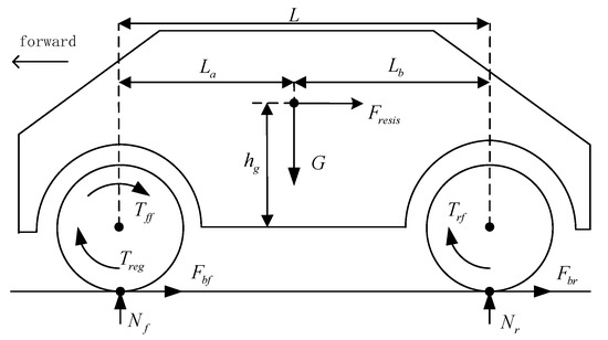
Figure 1. Forces acting on a vehicle while braking on the level ground [32].

Meanwhile, for $T_{reg}$, we have:

$$T_{reg}=F_{reg}r$$

(12)

where $r$ is the wheel radius and $F_{reg}$ is the regenerative braking force. The braking forces $F_{bf}$ and $F_{br}$ can then be written as [32]:

$$F_{bf \max }=\frac{\varphi G(L_b+z{h}_g)}{L}$$

(13)

$$F_{br \max }=\frac{\varphi G(L_a-z{h}_g)}{L}$$

(14)

where $F_{bf \max }$ and $F_{br \max }$ are the maximum braking forces acting on front and rear axles, respectively; $\varphi$ is the tire-ground adhesion coefficient, $z$ is the braking rate given by:

$$z=\frac{a}{g}$$

(15)

where $a$ is the deceleration of the vehicle, $g$ denotes the gravitational acceleration (9.8 N/kg). We can then express the deceleration $a$ as:

$$a=\frac{g(F_{bf}+F_{br}+F_{resis})}{G}.$$

(16)

with $G$ the weight of vehicle and $F_{resis}$ the resistance including air drag and force of friction.

In order to ensure the stability and the braking safety of the vehicle, the regulation (ECE-R13) established by the United Nations Economic Commission [33,34] suggests that the adhesion coefficients should satisfy the following relationships [32]:

$${\varphi }_f\ge {\varphi }_r$$

(17)

for $z\in [0.15, 0.8]$, and

$${\varphi }_f, {\varphi }_r\le \frac{z+0.07}{0.85}$$

(18)

for $z\in [0.1, 0.61]$, where ${\varphi }_f$ and ${\varphi }_r$ are the adhesion coefficients of front wheels and rear wheels, respectively.

Since electric motors features a wider operational range with higher efficiency compared to internal combustion engine, the conventional variable transmissions are not necessarily required. Then, in this paper, considering EV’s physical properties and braking safety, we formulate the EHB force allocation as the following NOP:

$$\begin{array}{l}\min f(x)\\ s.t. c_j(x)\le 0 j=1, ..., 11\end{array}$$

(19)

where $x={[F_{reg}, F_{ff}]}^T$, $f(x)=\frac{1}{1+F_{reg}^2}$ with constraints as:

$$\left\{\begin{array}{l}{c}_1(x)=F_{bf}-F_{bf \max }; c_2(x)=-F_{bf};\\ c_3(x)=F_{br}-F_{br \max }; c_4(x)=-F_{br};\\ c_5(x)={\varphi }_r-{\varphi }_f; (z\in [0.15, 0.8]) \\ c_6(x)={\varphi }_f-\frac{z+0.07}{0.85}; (z\in [0.1, 0.61])\\ c_7(x)={\varphi }_r-\frac{z+0.07}{0.85}; (z\in [0.1, 0.61]) \\ c_8(x)=T_{reg}-T_{reg \max }; c_9(x)={\omega }_m-{\omega }_{m \max }; \\ c_{10}(x)=-F_{reg}; c_{11}(x)=-F_{ff};\end{array}\right.$$

(20)

where ${\omega }_m$ and $P_m$ are the motor rotational speed and the motor power, bounded by ${\omega }_{m \max }$ and $P_{m \max }$, respectively.

The vehicle model is employed from the EV model in ADVISOR (Advanced Vehicle Simulator) software, where the RNN-NOPS is implemented as the braking strategy embedded in the vehicle control module. Important parameters of the considered vehicle given in ADVISOR are listed in Table 1, other parameters can also be found in the software. In this paper, the vehicle model is employed from the pure EV specified in ADVISOR, which is shown in Figure 2.

Table 1. Parameters of the considered vehicle.

Symbol	Meaning	Quantity
$m_v$	Vehicle mass	1144 kg
$m_c$	Vehicle cargo mass	136 kg
$h_g$	Height of the vehicle center of mass	0.5 m
$L$	Wheelbase	2.6 m
$L_a$	Longitudinal distance from the mass center to the front axle	1.04 m
$L_b$	Longitudinal distance from the mass center to the rear axle	1.56 m
$r$	Wheel radius	0.282 m
$F_A$	Frontal area	2 m2
$C_d$	Coefficient of aerodynamic drag	0.335
$f$	Coefficient of rolling resistance	0.009
$i_{gb}$	Ratio of the single speed transmission	2.9362

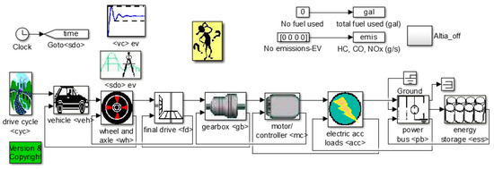
Figure 2. Pure EV model in ADVISOR.

3. RNN-NOPS Design

In this section, the design of RNN-NOPS is presented in detail. It will be shown that the RNN-NOPS is capable of driving the state variable that violates the constraints to converge to the feasible region with sufficient number of iterations, and KKT conditions hold at RNN-NOPS’s equilibria. Then the EHB force allocation problem will be confirmed to be solvable by using the RNN-NOPS.

3.1. Formulation of RNN-NOPS

In this section, the generalized framework of the RNN-NOPS is described as follows. Considering the NOP in Equation (1) with the Lagrangian function in Equation (2), the RNN-NOPS can be modelled by the following state equations:

$${\dot{x}}_i=-{\lambda }_1\left\{\frac{\partial f(x)}{\partial x_i}+{\displaystyle \sum _{k=1}^m\frac{\partial c_k(x)}{\partial x_i}\left[y_k+{(c_k(x))}^{+}\right]}\right\}$$

(21a)

$${\dot{y}}_k={\lambda }_2\left\{-y_k+{\left[y_k+\left(-2\cdot sign(c_k(x))+1\right)\cdot \left(-sign(y_k)-{(c_k(x))}^{+}\right)\right]}^{+}\right\}$$

(21b)

with:

$$\left\{\begin{array}{c}{x}_i(0)\in R, i=1, ..., n\\ y_k(0)\in R, k=1, ..., m\end{array}\right.$$

(21c)

where $x_i(0)$ and $y_k(0)$ are the initial values of $x_i$ and $y_k$, respectively, with the state vector $x$ defined as:

$$x={(x_i, ..., x_n)}^T$$

(22)

$y_k$ is the Lagrange multiplier corresponding to the constraint $c_k(x)$, ${(x_i)}^{+}=\max \{0, x_i\}$, ${(c_k(x))}^{+}=\max \{0, c_k(x)\}$, and $sign(\cdot )$ is the sign function, ${\lambda }_1$ and ${\lambda }_2$ are the positive learning rates.

Remark 2.

Because of the nonlinearity in Equation (21b), the stability of $y_k$can be analyzed piece-wisely as follows:

For $c_k(x)>0$:

Equation (21b) can be expressed as:

$${\dot{y}}_k={\lambda }_2\left\{-y_k+{\left[y_k+sign(y_k)+c_k(x)\right]}^{+}\right\}$$

(23)

If$y_k>0$,Equation (23) becomes:

$${\dot{y}}_k={\lambda }_2\left(1+c_k(x)\right)>0$$

(24a)

Equation (24a) indicates that $y_k\to \infty$as $t\to \infty$.

If$y_k=0$, Equation (23) can be written as:

$${\dot{y}}_k={\lambda }_2{c}_k(x)>0$$

(24b)

$y_k$will then move away from the origin $y_k=0$and go to infinity as time $t\to \infty$.

If $y_k<0$,Equation (23) is of the form:

$$\begin{array}{c}{\dot{y}}_k={\lambda }_2\left\{-y_k+{\left[y_k-1+c_k(x)\right]}^{+}\right\}\\ \hspace{1em}\hspace{1em}\hspace{1em}={\lambda }_2\left\{-y_k+{\left[-(\left|y_k\right|+1)+c_k(x)\right]}^{+}\right\}\end{array}$$

(24c)

In this case, $y_k$will move toward $y_k=0$.

The above analysis shows that, when the constraint $c_k(x)$is violated with $c_k(x)\ge 0$, the corresponding $y_k$either goes to infinity ($y_k\ge 0$) or converges to 0 ($y_k<0$).

For $c_k(x)=0$:

Equation (21b) becomes:

$${\dot{y}}_k={\lambda }_2\left\{-y_k+{\left[y_k-sign(y_k)\right]}^{+}\right\}$$

(25)

and then Equation (25) can be written as:

$$\begin{array}{l}{\dot{y}}_k={\lambda }_2\left[-y_k+{\left(y_k-1\right)}^{+}\right]\\ =\left\{\begin{array}{l}-{\lambda }_2<0, y_k>1\\ -{\lambda }_2{y}_k<0, 0<y_k\le 1\\ 0, \hspace{1em} y_k=0\\ {\lambda }_2>0, -1\le y_k<0\\ -{\lambda }_2{y}_k>0, y_k<-1\end{array}\right.\end{array}$$

(26a)

According to Lyapunov theory [35], Equation (26a) means that, with a selected Lyapunov function $V_{y_k}=0.5y_k^2$, we have:

$${\dot{V}}_{y_k}=y_k{\dot{y}}_k<0$$

(26b)

for $y_k\ne 0$, and ${\dot{V}}_{y_k}=0$if and only if $y_k=0$, therefore $y_k$can then asymptotically converge to zero.

Similarly, for $c_k(x)<0$, Equation (21b) can be written as:

$$\begin{array}{l}{\dot{y}}_k={\lambda }_2\left\{-y_k+{\left[y_k-3sign(y_k)\right]}^{+}\right\}\\ =\left\{\begin{array}{l}-3{\lambda }_2<0, \hspace{1em} y_k>3\\ -{\lambda }_2{y}_k<0, \hspace{1em}0<y_k\le 3\\ 0, \hspace{1em}\hspace{1em} y_k=0\\ 3{\lambda }_2>0, -3\le y_k<0\\ -{\lambda }_2{y}_k>0, -\infty \le y_k<-3\end{array}\right.\end{array}$$

(27)

Using Lyapunov stability theory, we can easily prove that, when the constraint $c_k(x)<0$, $y_k$asymptotically converges to zero. □

Assumptions 1.

For the NOP given by Equation (1), the following assumptions are made: (i) The partial derivative of objective $f(x)$with respect to $x_i$, $\frac{\partial f(x)}{\partial x_i}$, is bounded for all $i$; (ii) When $x$is out of the feasible region with $c_a(x)>0$, there always exists $x_i$making $\partial c_a(x)/\partial x_i\ne 0$holds, $i=1, ..., n$.

Based on the Assumptions 1, we have Proposition 1 as follows:

Proposition 1.

Consider the RNN-NOPS in Equation (21a–c) for solving the constrained NOP in Equations (1) and (2). If, a system state is out of the feasible region with the $a$th constraint violated, that is, $c_a(x)>0$, after sufficient number of iterations, RNN-NOPS will drive $x$to move to the feasible region satisfying $\frac{d{c}_a(x)}{dt}<0$, ensuring that all the constraints are within the feasible region.

Proof. 

Firstly, assuming that, at some sub-region of the state space, the $a$ th constraint is violated, that is, $c_a(x)>0$. According to Remark 2, if the corresponding $y_a$ we have ${\dot{y}}_a>0$; for other constraints with $c_k(x)\le 0$, after sufficient number of iterations, $y_k=0$. Then according to Equation (21a), any constraints $c_k(x)$ satisfying $c_k(x)\le 0$, have no effect on the updates on $x_i$. Therefore, after sufficient number of iterations, Equation (21a) becomes:

$$\begin{array}{l}{\dot{x}}_i=-{\lambda }_1\left\{\frac{\partial f(x)}{\partial x_i}+{\displaystyle \sum _{k=1}^m\left[\frac{\partial c_k(x)}{\partial x_i}\left(y_k+{(c_k(x))}^{+}\right)\right]}\right\}\\ =-{\lambda }_1\left\{\frac{\partial f(x)}{\partial x_i}+\frac{\partial c_a(x)}{\partial x_i}\left[y_a+{(c_a(x))}^{+}\right]\right\}\end{array}$$

(28)

Since $\frac{\partial f(x)}{\partial x_i}$ is assumed to be bounded, when the violated constraint $c_a(x)>0$ makes ${\dot{y}}_a>0$, $y_a$ will continuously increase such that, after a large number of iterations, the following inequality is held:

$$\left|\frac{\partial c_a(x)}{\partial x_i}\left[y_a+{(c_a(x))}^{+}\right]\right|\gg \left|\frac{\partial f(x)}{\partial x_i}\right|$$

(29)

then we have:

$${\dot{x}}_i\approx -{\lambda }_1\frac{\partial c_a(x)}{\partial x_i}\left[y_a+{(c_a(x))}^{+}\right]$$

(30)

Equation (30) means that all $x_i$ will move approximately along the negative gradient direction of $c_a(x)$, which is similar to gradient descent approach, and the positive ${\lambda }_1\left[y_a+{(c_a(x))}^{+}\right]$ in Equation (28) can be regarded as updating step size. From Assumptions 1, $\exists x_i$ making $\partial c_a(x)/\partial x_i\ne 0$ holds, and then

$${\dot{x}}_i\frac{\partial c_a(x)}{\partial x_i}\approx -{\lambda }_1{\left(\frac{\partial c_a(x)}{\partial x_i}\right)}^2\left[y_a+{(c_a(x))}^{+}\right]<0, i=1, ..., n$$

(31)

Adding $n$ equations of Equation (31) for $i=1, ..., n$, we obtain:

$$\begin{array}{l}\frac{d{c}_a(x)}{dt}={\displaystyle \sum _{i=1}^n\left[{\dot{x}}_i(\frac{\partial c_a(x)}{\partial x_i})\right]}\\ \approx -{\lambda }_1{\displaystyle \sum _{i=1}^n\left\{{\left(\frac{\partial c_a(x)}{\partial x_i}\right)}^2\left[y_a+{(c_a(x))}^{+}\right]\right\}}<0\end{array}$$

(32)

Equation (32) means that there exists a time $t_0$, with $t>t_0$, we have $c_k(x)\le 0$. □

Remark 3.

It is seen from Proposition 1 that the RNN-NOPS proposed in this paper has the following remarkable robustness and convergence properties:

(i) If the state variable vector is out of the feasible region with some constraint violated ($c_a(x)>0$), the RNN-NOPS is capable of continuously increasing the values of the corresponding Lagrangian multipliers (the state variables) such that, after a number of iterations with the large variable step sizes, the changing rate of the violated constraints becomes negative ($c_a(x)>0$). This process is named as the “constraint recovering process”;

(ii) After all constraints are valid within the feasible region, the RNN-NOPS drives all Lagrangian multipliers to converge to zero ($y_k=0$) in the Lyapunov sense. Then the original constrained optimization, as specified in Equation (1), behaves as an unconstrained optimization. This process can be considered as the “objective optimizing process”.

3.2. KKT Condition and Convergence Analysis

In this section, two theorems regarding RNN-NOPS’s convergence and optimality are presented.

Theorem 1.

Consider the RNN-NOPS in Equation (21a–c) for solving the constrained NOP in Equations (1) and (2). If $(x,y)$is an equilibrium of the RNN-NOPS, $(x,y)$is a KKT point of the optimization problem.

Proof. 

Let $(x^{*},y^{*})$ be a KKT point, from Equation (3) we have:

$$\left\{\begin{array}{l}\nabla f(x^{*})+{\displaystyle \sum _{k=1}^m\nabla c_k(x^{*})y_k^{*}}=0\\ c_k(x^{*})y_k^{*}=0\\ y_k^{*}\ge 0\\ c_k(x^{*})\le 0\end{array}\right.$$

(33)

where $x_i^{*}\ge 0$ is included in $c_k(x^{*})\le 0$.

Given $(x,y)$ is an equilibrium with ${\dot{x}}_i={\dot{y}}_k=0$, according to Remark 2, ${\dot{y}}_k=0$ is met only if $c_k(x)\le 0$, then given ${\dot{y}}_k=0$ we have $c_k(x)\le 0$, that is the 4th KKT condition in Equation (33) is met.

According to Remark 2, when $c_k(x)\le 0$, $y_k$ is only stable at $y_k=0$, so given ${\dot{y}}_k=0$, $y_k=0$ is obtained, that is the 3rd KKT condition in Equation (33) is satisfied.

Given $(x,y)$ is an equilibrium, ${\dot{x}}_i=0$ for all $i$, then Equation (21a) yields:

$$\begin{array}{l} {\lambda }_1\left\{\frac{\partial f(x)}{\partial x_i}+{\displaystyle \sum _{k=1}^m\left[\frac{\partial c_k(x)}{\partial x_i}\left(y_k+{(c_k(x))}^{+}\right)\right]}\right\}\\ ={\lambda }_1\left[\frac{\partial f(x)}{\partial x_i}+{\displaystyle \sum _{k=1}^m\left(\frac{\partial c_k(x)}{\partial x_i}{y}_k\right)}\right]\\ =0\end{array}$$

(34)

that is, the 1st KKT condition in Equation (33) is satisfied.

Finally, from $c_j(x)\le 0$ along with Remark 2, $y_j$ is stable only if $y_j=0$, then $y_j=0$ and $c_j(x)y_j=0$, that is, the 2nd KKT condition in Equation (33) holds.

Thereby, the proof is finished. □

Remark 4.

Based on the Lyapunov theory along with Assumptions 1, the convergence of RNN-NOPS is ready to be investigated. Firstly, a constraint mapping variable $w={[w_1, ..., w_k, ..., w_m]}^T$is defined with $w_k={(c_k(x))}^{+}$, then $w_k=0$given $c_k(x)\le 0$; and according to Remark 2, $y_k$is stable only if $y_k=0$and $c_k(x)\le 0$.

For a constraint recovering process, there is single equilibrium $0$ at the space ${\mathfrak{R}}^m$ where $w$ locates. $0$ can be seen as the mapping of the whole feasible region, therefore for the upcoming objective optimizing process, $w$ is stable at $w=0$. Then, the theorem on RNN-NOPS’s convergence is given as follows:

Theorem 2.

For a whole solving process of RNN-NOPS consisting of one constraints recovering process and one objective optimization process, on the basis of Assumptions 1, when there is one constraint $c_a(x)>0$,$0$in ${\mathfrak{R}}^m$where $w$locates is asymptotically stable.

Proof. 

Consider a Lyapunov function $V$:

$$V=\frac{1}{2}{w}^{T}w$$

(35)

where $w={[w_1, ..., w_k, ..., w_m]}^T$, $w_k={(c_k(x))}^{+}$, we have $V\ge 0$ and $V$ is radically unbounded. When the state vector $x$ is within the feasible region $\Omega =\left\{x\right|c_k(x)\le 0, k=1, ..., m\}$, $w$ is stable at ${\mathfrak{R}}^m$ space equilibrium $0$ and $V=0$, $V$ reaches its minimum value. Then we have:

$$V=\frac{1}{2}{\displaystyle \sum _{k=1}^m{w}_k^2}$$

(36)

And

$$\dot{V}={\displaystyle \sum _{k=1}^m{w}_k}\frac{d{w}_k}{dt}$$

(37)

where $\dot{V}$ is the sum of $m$ terms, $w_k=0$ when $c_j(x)\le 0$. Only if there is $c_a(x)>0$, there could be $w_a{\dot{w}}_a\ne 0$, and in this case we also have $w_a=c_a(x)$ and ${\dot{w}}_a=\frac{d{c}_a(x)}{dt}$. That is, the value of $\dot{V}$ is determined by $c_a(x)$ and its corresponding multiplier $y_a$:

$$\dot{V}=w_a{\dot{w}}_a=c_a(x)\frac{d{c}_a(x)}{dt}$$

(38)

According to Proposition 1, $c_a(x)>0$ makes its corresponding $y_a$ keeps increasing until sufficiently large, making Equation (38) hold, that is $\frac{d{c}_a(x)}{dt}<0$, then we have:

$$\dot{V}=c_a(x)\frac{d{c}_a(x)}{dt}<0$$

(39)

Therefore, equilibrium $0$ in ${\mathfrak{R}}^m$ space where $w$ locates is globally asymptotically stable.

Thereby, the proof is finished. □

Remark 5.

The convergence properties discussed in the above are based on Assumptions 1, where the first condition could be easily realized by properly constructing the objective function. For example, if $f(x)=\frac{1}{F_{reg}^2}$instead of $f(x)=\frac{1}{1+F_{reg}^2}$, the $\partial f(x)/\partial x_i\to \infty$when $F_{reg}=0$. The second condition in the Assumptions 1 is also mild and valid for the optimization problem formulated in Equations (19) and (20).

3.3. Analysis of the NOP to Be Solved

In this section, the EHB force allocation problem in NOP form is verified to fit Assumptions 1.

Remark 6.

The partial derivatives of $f(x)$and $c_j(x)$,$j=1, ..., m$with respect to $F_{reg}$and$F_{ff}$are given in Table 2. Substituting the parameters’ values, it is seen that the denominator of $\partial f(x)/\partial F_{reg}$is always positive and the numerator is bounded, and that $\partial f(x)/\partial F_{ff}=0$. Meanwhile, for any $c_k(x)$, $\partial f(x)/\partial F_{reg}$and$\partial f(x)/\partial F_{ff}$are not equal to 0 at the same time. For example,$\partial c_5(x)/\partial F_{reg}=\partial c_5(x)/\partial F_{ff}=0$if and only if $L_a-h_{g}z=-\left(L_b+h_{g}z\right)$, and there is no solution for$z$. Therefore, conditions in Assumptions 1 are all satisfied. It is also worth noting that the only exception, $c_9(x)$, is always satisfied with the driving cycle not exceeding the operating limit of the vehicle, therefore $c_9(x)$has no effect on the update of state variables.

Table 2. First order partial derivative of the objective function and constraints with respect to $x_i$.

$\partial f(x)/\partial F_{reg}$	$\partial c_1(x)/\partial F_{reg}$	$\partial c_2(x)/\partial F_{reg}$	$\partial c_3(x)/\partial F_{reg}$	$\partial c_4(x)/\partial F_{reg}$	$\partial c_5(x)/\partial F_{reg}$
$-\frac{2F_{reg}}{{\left(F_{reg}^2+1\right)}^2}$	1	−1	−1	1	$-\frac{L}{G\left(L_a-h_{g}z\right)}-\frac{L}{G\left(L_b+h_{g}z\right)}$
$\partial c_6(x)/\partial F_{reg}$	$\partial c_7(x)/\partial F_{reg}$	$\partial c_8(x)/\partial F_{reg}$	$\partial c_9(x)/\partial F_{reg}$	$\partial c_{10}(x)/\partial F_{reg}$	$\partial c_{11}(x)/\partial F_{reg}$
$\frac{L}{G\left(L_b+h_{g}z\right)}$	$-\frac{L}{G\left(L_a-h_{g}z\right)}$	1	0	−1	0
$\partial f(x)/\partial F_{ff}$	$\partial c_1(x)/\partial F_{ff}$	$\partial c_2(x)/\partial F_{ff}$	$\partial c_3(x)/\partial F_{ff}$	$\partial c_4(x)/\partial F_{ff}$	$\partial c_5(x)/\partial F_{ff}$
0	1	−1	−1	1	$-\frac{L}{G\left(L_a-h_{g}z\right)}-\frac{L}{G\left(L_b+h_{g}z\right)}$
$\partial c_6(x)/\partial F_{ff}$	$\partial c_7(x)/\partial F_{ff}$	$\partial c_8(x)/\partial F_{ff}$	$\partial c_9(x)/\partial F_{ff}$	$\partial c_{10}(x)/\partial F_{ff}$	$\partial c_{11}(x)/\partial F_{ff}$
$\frac{L}{G\left(L_b+h_{g}z\right)}$	$-\frac{L}{G\left(L_a-h_{g}z\right)}$	0	0	0	−1

4. Simulations and Discussion

In this section, the comparative study of the EHB force allocation problem is carried out under both predefined braking process and standard driving cycle. The aforementioned extended projection neural network (EPNN) [16] is implemented as comparison.

4.1. Learning Performance Evaluation

In this section, EHB force allocation strategies are conducted in the EV under a designed braking process, with the initial speed set as 18 m/s, the acceleration set as −1 m/s² in 1–4 s, −2 m/s² in 4–7 s and −3 m/s² in 7–10 s, and the EV is stationary at the 10th second. By doing this, the strategy can be validated under various velocities and braking rates.

The simulation step is set as 0.1 s. At every simulation step, RNN-NOPS and EPNN are aligned 5 × 10⁴ iterations to make sure the training is sufficient. The learning rates of RNN-NOPS are set as ${\lambda }_1={\lambda }_2=0.04$, as for EPNN, $\alpha =0.42$, $y_k$ are all initialized as 0. $F_{reg}$ and $F_{ff}$ are initialized as −100, respectively, making $c_5(x)>0$ at some steps with $z\in [0.1, 0.61]$, so that the training process of all networks must take constraints into consideration.

The speed of the designed braking process and the EV’s actual speed with RNN-NOPS are shown in Figure 3, where it is shown that the vehicle speed under control of RNN-NOPS follows the target speed with delay and the overall trends are consistent. Speed following results with EPNN are similar.

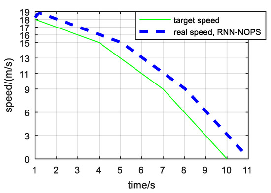
Figure 3. Speed of the EV during the braking process under control of RNN-NOPS.

Take 2 representative constraints, $c_5(x)$ and $c_6(x)$ as examples, their 59 training trajectories (representing 59 training sample times considering $c_5(x)$ and $c_6(x)$) at first 5 × 10⁴ iterations of RNN-NOPS and EPNN are shown in Figure 4. It is seen that $c_5(x)$ is often positive at initial iterations, representing ${\varphi }_r$ exceeds ${\varphi }_f$. Since the braking ratio is fixed at every step, according to Equation (20), increasing ${\varphi }_f$ is the feasible way to recover the violated $c_5(x)$, which means $c_6(x)$ must be increased. From Figure 4b,d, it is seen that negative $c_6(x)$ is increased but within its feasible range, indicating that all the algorithms effectively find a way to recover violated constraints.

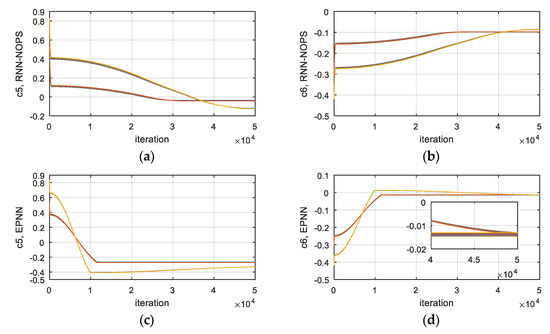
Figure 4. $c_5(x)$ and $c_6(x)$ ’s trajectories of (a), (b) RNN-NOPS and (c), (d) EPNN, respectively.

Overall results during the designed braking process are shown in Table 3, where it is shown that all the constraints are perfectly obeyed by both algorithms. With regard to the overall regenerative energy, RNN-NOPS recovers 6.77% more energy than EPNN.

Table 3. Overall results under the designed braking process in terms of regenerative energy and constraint violation.

	RNN-NOPS	EPNN
Overall regenerative energy (J)	5.3954 × 104	5.0532 × 104
Overall constraint violation	0	0

4.2. Braking Performance Evaluation

It is found that for both strategies, the braking time is from 1.3 s to 10.9 s. The braking results are shown in Figure 5, where the following observations can be seen:

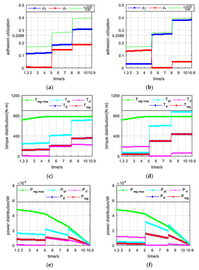
Figure 5. Braking performance of RNN-NOPS and EPNN in terms of adhesion utilization in (a,b), respectively; torque allocation in (c,d), respectively; power allocation in (e,f), respectively.

(i) Adhesion utilization results of RNN-NOPS and EPNN are shown in Figure 5a,b, respectively. When $z=0.1$, $(z+0.07)/0.85=0.2$; when $z=0.15$, $(z+0.07)/0.85$ is about 0.2588. Then from Equation (20), given $(z+0.07)/0.85<0.2588$, $c_5(x)$ is not involved in the NOP and ${\varphi }_r>{\varphi }_f$ is allowed; and when $(z+0.07)/0.85<0.2$, $c_6(x)$ and $c_7(x)$ are not considered and ${\varphi }_f, {\varphi }_r>(z+0.07)/0.85$ is allowed.

The $c_5(x)$ is not involved in 1.3–5.0 s, so it is seen from Figure 5a,b that ${\varphi }_r>{\varphi }_f$ during this time. The difference is that in this case, ${\varphi }_r$ of RNN-NOPS is much lower than that of EPNN, indicating that RNN-NOPS decreases torque consumed by friction on the rear axle and brings more energy on the front axle for possible regeneration.

The $z$ is higher in 5.1–10.9 s, when $c_5(x)$, $c_6(x)$ and $c_7(x)$ are all involved. EPNN concentrates more torque on front axle at this time.

(ii) Torque allocation results of RNN-NOPS and EPNN are shown in Figure 5c,d, respectively. It is seen that $T_{reg}\le T_{reg \max }$ holds for both algorithms, $T_{ff}$ and $T_{reg}$ are close in both pictures. However, in 1–4 s, $T_{reg}$ of EPNN is almost 0, while that of RNN-NOPS is much higher. This is because EPNN tends to allocate more braking force/torque to the rear axle, where all energy is dissipated by friction of hydraulic braking. This result explains the different regenerative energy of both algorithms.

(iii) Power allocation results of RNN-NOPS and EPNN are shown in Figure 5e,f, respectively. It is seen that, as the braking process tends to complete, the rotational speed of the motor decreases, which makes the energy available for regeneration decrease. At this time, EPNN concentrates more torque on front axle but does not regenerate much more energy than RNN-NOPS. This is verified by the results in Table 3.

4.3. Performance under Standard Driving Cycle

In this section, the comparative study with a few existing RNN algorithms for solving NOPs is conducted under a standard driving cycle, which reflects the practical environment and the driver’s behavior.

SC03 Supplemental Federal Test Procedure (SFTP) is a testing cycle proposed by the Environmental Protection Agency (EPA) in 2007, and it is chosen as the testing cycle in this section. The simulation step size is set as 1 s, where 1 × 10⁴ iterations are allocated for both algorithms. The learning rates of RNN-NOPS are selected as ${\lambda }_1={\lambda }_2=0.32$, and $\alpha =2$ in EPNN. Other settings are similar to Section 4.1.

The speed-following results are shown in Figure. 6, where the speed of SC03 and speed under control of RNN-NOPS are shown in Figure 6a, and the speed-following error is shown in Figure 6b. It is seen that SC03 is well-followed.

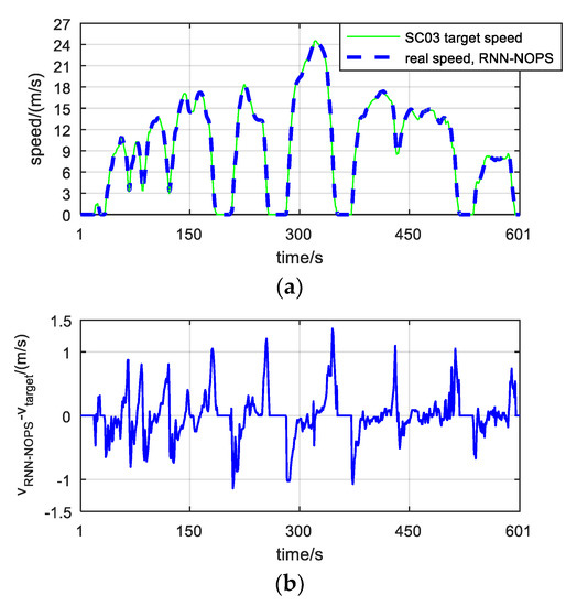
Figure 6. SC03 speed and real speed under control of RNN-NOPS in (a), and speed-following error in (b).

The trajectories of $c_5(x)$ and $c_6(x)$ are shown in Figure 7, where the results of RNN-NOPS are illustrated in Figure 7a,b, and those of EPNN are shown in Figure 7c,d. The first 600 iterations of RNN-NOPS and 8000 iterations of EPNN are given, respectively. In Figure 7a,c, 13 training trajectories representing 13 sample times with $z\in [0.15, 0.8]$ considering $c_5(x)$, are given, respectively. In Figure 7a,c, 34 training trajectories representing 34 sample times with $z\in [0.1, 0.61]$ considering $c_6(x)$, are given, respectively. Initial $c_5(x)$ is sometimes violated, and finally the trajectories are all stable at valid negative values for both algorithms, indicating reliable learning performance.

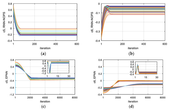
Figure 7. Trajectories during training process of RNN-NOPS and EPNN under SC03 cycle in terms of constraint 5 in (a) and (c), respectively, and constraint 6 in (b) and (d), respectively.

Finally, the overall results in terms of regenerative energy and constraint violation are shown in Table 4, where it is seen that all constraints are obeyed for both algorithms. Yet the overall regenerative energy of RNN-NOPS is 15.39% more than that of EPNN.

Table 4. Results of algorithms under SC03 in terms of regenerative energy and constraint violation.

	RNN-NOPS	EPNN
Overall regenerative energy (J)	1.3822 × 105	1.1978 × 105
Overall constraint violation	0	0

5. Conclusions

In this paper, an RNN-NOPS has been proposed and applied for EHB force allocation of EVs. The RNN-NOPS has been designed to ensure that the state variables converge to the feasible region and the equilibria meet KKT conditions of the NOP. The network’s update consists of two processes dealing with constraints and the objective function, respectively. It is reported that the overall regenerative energy of RNN-NOPS is 15.39% more than that of the method for comparison under SC03 cycle. The main benefits of the proposed RNN-NOPS are threefold: (1) The RNN-based method with parallel computation is suitable for timely industrial applications; (2) Guaranteed optimality can be obtained by RNN-NOPS with the constraints met, with a requirement on the first-order partial derivative of the NOP; (3) The simulation results of the EHB force allocation problem under different braking processes have demonstrated the excellent performance of the RNN-NOPS regarding the convergence, braking safety, regenerative energy, etc. Yet the limitation of RNN-NOPS is that the solving result is sensitive to parameters setting; not all constraints are satisfied before convergence with an inappropriate learning rate. The further work on RNN-based NOP-solving models aims at broadening the application scope with reduced model complexity and less sensitivity to parameters.

References

- Gao, Y.; Chen, L.; Ehsani, M. Investigation of the Effectiveness of Regenerative Braking for EV and HEV; SAE Transactions: Warrendale, PA, USA, 1999; pp. 3184–3190. [Google Scholar]
- Kim, D.H.; Kim, J.M.; Hwang, S.H.; Kim, H.S. Optimal brake torque distribution for a four-wheel drive hybrid electric vehicle stability enhancement. Proc. Inst. Mech. Eng. Part D J. Automob. Eng. 2007, 221, 1357–1366. [Google Scholar] [CrossRef]
- Katoch, S.; Chauhan, S.S.; Kumar, V. A review on genetic algorithm: Past, present, and future. Multimed. Tools Appl. 2021, 80, 8091–8126. [Google Scholar] [CrossRef] [PubMed]
- Satzger, C.; de Castro, R. Predictive brake control for electric vehicles. IEEE Trans. Veh. Technol. 2017, 67, 977–990. [Google Scholar] [CrossRef]
- Behrooz, F.; Mariun, N.; Marhaban, M.H.; Radzi, M.A.M.; Ramli, A.R. Review of control techniques for HVAC systems—nonlinearity approaches based on fuzzy cognitive maps. Energies 2018, 11, 495. [Google Scholar] [CrossRef]
- Liu, Q.; Guo, Z.; Wang, J. A one-layer recurrent neural network for constrained pseudoconvex optimization and its application for dynamic portfolio optimization. Neural Netw. 2012, 26, 99–109. [Google Scholar] [CrossRef]
- Cui, X.; Li, X.; Li, D. Unified framework of mean-field formulations for optimal multi-period mean-variance portfolio selection. IEEE Trans. Autom. Control 2014, 59, 1833–1844. [Google Scholar] [CrossRef]
- Leung, M.-F.; Wang, J. Minimax and biobjective portfolio selection based on collaborative neurodynamic optimization. IEEE Trans. Neural Netw. Learn. Syst. 2020, 32, 2825–2836. [Google Scholar] [CrossRef]
- Pan, Y.; Wang, J. Model predictive control of unknown nonlinear dynamical systems based on recurrent neural networks. IEEE Trans. Ind. Electron. 2011, 59, 3089–3101. [Google Scholar] [CrossRef]
- Yan, Z.; Wang, J. Robust model predictive control of nonlinear systems with unmodeled dynamics and bounded uncertainties based on neural networks. IEEE Trans. Neural Netw. Learn. Syst. 2013, 25, 457–469. [Google Scholar] [CrossRef]
- Yan, Z.; Wang, J. Nonlinear model predictive control based on collective neurodynamic optimization. IEEE Trans. Neural Netw. Learn. Syst. 2015, 26, 840–850. [Google Scholar] [CrossRef]
- Peng, Z.; Wang, J.; Wang, D. Distributed maneuvering of autonomous surface vehicles based on neurodynamic optimization and fuzzy approximation. IEEE Trans. Control. Syst. Technol. 2017, 26, 1083–1090. [Google Scholar] [CrossRef]
- Xia, Y.; Wang, J. A One-layer recurrent neural network for support vector machine learning. IEEE Trans. Syst. Man Cybern. Part B (Cybernetics) 2004, 34, 1261–1269. [Google Scholar] [CrossRef] [PubMed]
- Solodov, M.V.; Tseng, P. Modified projection-type methods for monotone variational inequalities. SIAM J. Control Optim. 1996, 34, 1814–1830. [Google Scholar] [CrossRef]
- Konnov, I.V. A Class of combined iterative methods for solving variational inequalities. J. Optim. Theory Appl. 1997, 94, 677–693. [Google Scholar] [CrossRef]
- Xia, Y.; Wang, J. A Recurrent neural network for nonlinear convex optimization subject to nonlinear inequality constraints. IEEE Trans. Circuits Syst. I Regul. Pap. 2004, 51, 1385–1394. [Google Scholar] [CrossRef]
- Xia, Y.; Feng, G.; Wang, J. A novel recurrent neural network for solving nonlinear optimization problems with inequality constraints. IEEE Trans. Neural Netw. 2008, 19, 1340–1353. [Google Scholar]
- Tank, D.; Hopfield, J. Simple ‘neural’ optimization networks: An A/D converter, signal decision circuit, and a linear programming circuit. IEEE Trans. Circuits Syst. 1986, 33, 533–541. [Google Scholar] [CrossRef]
- Khan, N.; Haq, I.U.; Ullah FU, M.; Khan, S.U.; Lee, M.Y. CL-Net: ConvLSTM-Based Hybrid Architecture for Batteries’ State of Health and Power Consumption Forecasting. Mathematics 2021, 9, 3326. [Google Scholar] [CrossRef]
- Chen, R.T.; Rubanova, Y.; Bettencourt, J.; Duvenaud, D.K. Neural ordinary differential equations. Adv. Neural Inf. Process. Syst. 2018, 31, 6572–6583. [Google Scholar]
- He, K.; Zhang, X.; Ren, S.; Sun, J. Deep residual learning for image recognition. In Proceedings of the IEEE Conference on Computer Vision and Pattern Recognition, Las Vegas, NV, USA, 27–30 June 2016; pp. 770–778. [Google Scholar]
- Tkachenko, R.; Izonin, I.; Vitynskyi, P.; Lotoshynska, N.; Pavlyuk, O. Development of the non-iterative supervised learning predictor based on the ito decomposition and SGTM neural-like structure for managing medical insurance costs. Data 2018, 3, 46. [Google Scholar] [CrossRef]
- Li, G.; Yan, Z.; Wang, J. A one-layer recurrent neural network for constrained nonconvex optimization. Neural Netw. 2015, 61, 10–21. [Google Scholar] [CrossRef]
- Che, H.; Wang, J. A collaborative neurodynamic approach to global and combinatorial optimization. Neural Netw. 2019, 114, 15–27. [Google Scholar] [CrossRef] [PubMed]
- Bazaraa, M.S.; Sherali, H.D.; Shetty, C.M. Nonlinear Programming: Theory and Algorithms; John Wiley & Sons: Hoboken, NJ, USA, 2013. [Google Scholar]
- Xia, Y.; Wang, J.; Guo, W. Two projection neural networks with reduced model complexity for nonlinear programming. IEEE Trans. Neural Netw. Learn. Syst. 2019, 31, 2020–2029. [Google Scholar] [CrossRef] [PubMed]
- Granville, S.; Rodrigo de Miranda Alves, F. Active-reactive coupling in optimal reactive dispatch: A solution via Karush-Kuhn-Tucker optimality conditions. IEEE Trans. Power Syst. 1994, 9, 1774–1779. [Google Scholar] [CrossRef]
- Huang, Y. Lagrange-type neural networks for nonlinear programming problems with inequality constraints. In Proceedings of the 44th IEEE Conference on Decision and Control, Seville, Spain, 15 December 2005; pp. 4129–4133. [Google Scholar]
- La Salle, J.P. The Stability of Dynamical Systems; Society for Industrial and Applied Mathematics: Philadelphia, PA, USA, 1976. [Google Scholar]
- Xia, Y.; Leung, H.; Wang, J. A projection neural network and its application to constrained optimization problems. IEEE Trans. Circuits Syst. I Fundam. Theory Appl. 2002, 49, 447–458. [Google Scholar]
- Dall'Anese, E.; Simonetto, A.; Becker, S.; Madden, L. Optimization and learning with information streams: Time-varying algorithms and applications. IEEE Signal Process. Mag. 2020, 37, 71–83. [Google Scholar] [CrossRef]
- Guo, J.; Wang, J.; Cao, B. Study on braking force distribution of electric vehicles. In Proceedings of the 2009 Asia-Pacific Power and Energy Engineering Conference, Wuhan, China, 27–31 March 2009; pp. 1–4. [Google Scholar]
- Ma, K.; Chu, L.; Yao, L.; Wang, Y. Study on control strategy for regenerative braking in a pure electric vehicle. In Proceedings of the 2nd International Conference on Electronic & Mechanical Engineering and Information Technology, Shenyang, China, 7 September 2012; pp. 1875–1878. [Google Scholar]
- ECE/324/Rev.1/Add.12/Rev.8, Addendum 12: Regulation No.13, Agreement Concerning the Adoption of Uniform Technical Prescriptions for Wheeled Vehicles, Equipment and Parts which can be Fitted and/or be Used on Wheeled Vehicles and the Conditions for Reciprocal Recognition of Approvals Granted on the Basis of these Prescriptions. United Nations. 3 March 2014. Available online: https://www.unece.org/fileadmin/DAM/trans/main/wp29/wp29regs/updates/R013r8e.pdf (accessed on 10 February 2021).
- Khalil, H. Nonlinear Systems; Prentice-Hall: Hoboken, NJ, USA, 2002. [Google Scholar]
Publisher’s Note: MDPI stays neutral with regard to jurisdictional claims in published maps and institutional affiliations. |
© 2022 by the authors. Licensee MDPI, Basel, Switzerland. This article is an open access article distributed under the terms and conditions of the Creative Commons Attribution (CC BY) license (https://creativecommons.org/licenses/by/4.0/).