Abstract
The radioactive gas radon is ubiquitous in the environment and is a major contributor to the human inhalation dose. It is the second leading cause of lung cancer after smoking. Radon concentrations are particularly high in the air of radon-hazardous facilities—uranium mines and radioactive waste repositories containing radium. To reduce the dose load on the staff, air in these premises should be continuously or periodically purified of radon. Carbon adsorbers can be successfully used for this purpose. The design of sorption systems requires information on both equilibrium and kinetic parameters of radon dynamic adsorption. The traditional way of obtaining such characteristics of the sorbent is to analyze the breakthrough curves. The present paper proposes a simple alternative method for determining parameters of dynamic radon adsorption (Henry’s constant and equilibrium adsorption layer thickness) from the results of a layer-by-layer gamma-spectrometric measurement of the sorbent. The analytical equation for smooth distribution of radon activity in the sorbent layer is obtained based on equilibrium adsorption layer theory for elute chromatography (pulsed injection of radon into the column). Using the dynamic adsorption of 222Rn on AG-3 activated carbon as an example, both equilibrium (Henry’s constant) and kinetic (thickness of the equilibrium adsorption layer) parameters of the adsorption dynamics were calculated. It was shown that the exposure duration of the column bed in the air flow and superficial gas velocity do not affect the result of the Henry’s constant calculation. The dependence of the equilibrium adsorption layer thickness on the superficial gas velocity over a wide range of values (5–220 cm/min) is described by the van Deemter equation. It was shown that the optimum air flow velocity, which corresponds to the maximum effectiveness of the bed, is 15–30 cm/min. This corresponds to the minimum of the equilibrium adsorption layer thickness (about 0.6 cm). The developed mathematical model makes it easy to define both equilibrium and kinetic parameters of dynamic adsorption of radon based on discrete distribution of its activity over the sections of the adsorption column. These parameters can then be used to calculate and design gas delay systems. It can be useful for studying the sorption capacity of various materials relative to radon.
1. Introduction
The problem of radon is global since the longest-lived isotope—222Rn—is part of the natural radioactive family 238U and is distributed almost everywhere. This radioactive gas makes the main contribution to the collective radiation dose of the population. According to [1], worldwide the average annual dose of radiation to the population consists of medical irradiation (21%), man-made (1%), and natural (79%), the bulk of which (52–54%) is due to inhalation of air containing radon isotopes and their decay products. The national average individual annual effective radiation dose to the population due to all natural sources of radiation is about 3.4 mSv/y, and most of it is formed due to irradiation of the population with radon isotopes in indoor air—an average of about 58% [1]. Thus, the exposure of radon to the population is significantly higher than that due to man-caused and medical sources of ionizing radiation. There is now a rich source of experimental data and long-term observations showing a link between the lung cancer risks and inhalation of radon and its decay products [2].
The main sources of radon in civilian facilities are natural water, the soil under the building, natural gas, and construction materials containing 226Ra and 232Th. The main man-made sources of radon are uranium mines, radioactive waste (RAW), and spent nuclear fuel (SNF) storage facilities. Radon enters the air of these facilities from uranium and thorium compounds located there, as well as decommissioned radium sources of gamma radiation. Since in such underground structures the surrounding rocks and materials constantly emit significant amounts of radon, forced ventilation is ineffective in reducing its concentration. The simplest and most effective way to purify air from radon can be considered the adsorption method, since the sorption capacity of several industrial adsorbents (such as activated carbons) in relation to radon is quite high [3].
Radon adsorption on activated carbon is quite widely covered in the scientific literature [3,4,5,6,7]. However, most publications are confined to calculating adsorption coefficients (Henry’s constants) under static or dynamic conditions. Papers describing the quantitative characteristics of the radon dynamic adsorption are much less [8]. No matter how accurately the radon adsorption coefficient is known, without factors describing the radon mass transfer process inside the adsorption bed, it is impossible to say how well the adsorbent will work. This is important to consider, for example, in the design or calculation of a cyclic radon removal system. Thus, to obtain a complete characteristic of the suitability of a particular adsorbent, it is necessary to know both equilibrium and kinetic adsorption parameters.
The traditional way to calculate the parameters of radon adsorption is the mathematical processing of the breakthrough curve—the time dependence of the volumetric activity of radon in the air, leaving the column. Typically, the radon breakthrough curve is obtained for the frontal adsorption mode when radon is continuously fed into the air stream. This embodiment of the experiment requires a constantly operating source of radon of sufficient volumetric activity. For this purpose, so-called radon rooms (chambers) are usually used, i.e., large-volume containers (usually as large as several cubic meters) containing radon-emanating materials [3,4,6,9]. In some works, other sources of radon are described: in [10], air containing radon was supplied by a diaphragm pump from the soil outside the laboratory from a depth of 1 m, and in [7] the air flow was saturated with radon, bubbling a solution of radium chloride. There is a known method for producing radon by passing air over a melt of radium salt in a eutectic [11]. None of these methods can be considered convenient enough and suitable for wide application in research laboratories.
The parameters of the dynamic adsorption of radon (Henry’s constant, kinetic coefficient) can also be obtained by mathematical processing of an elution breakthrough curve. Unlike the frontal variant of adsorption, such an experiment involves a short-pulse injection of radon into the air flow passing through the sorbent. This makes it possible to significantly reduce the requirements for the activity of the radon source and simplify its design. In fact, the simplest and most suitable method for the pulsed injection of radon into the adsorption column seems to be an isotope periodic generator, in which the required amount of radon is formed during the decay of 226Ra in periods between experiments. However, even in this case, the experimental facility for studying radon adsorption should include radiometric equipment—a flow-through particle counter or a gamma-spectrometer. The need to measure the volumetric activity of the air flow complicates the installation scheme and imposes some restrictions on the concentration of radon in the input pulse: it must be sufficient to reliably measure the activity of the air flow in real time (continuously or periodically). In addition, deposition on the flow-through detector of alpha- and gamma-emitting decay products of radon can lead to distortion of the shape of the breakthrough curve. In [8], the authors had to compensate this effect using sophisticated mathematical processing of the detector signal in experiments with the passage of radon through the adsorbent bed and in parallel idle experiments (without an adsorbent).
Layer-by-layer measurement of radon activity or its daughter decay products in the sorbent has several advantages over continuous radiometry of the air flow. In this version, expensive equipment is excluded from the hardware scheme of the experimental facility. The duration of the experiment can also be reduced several times. Radiometry of the sorbent and the conduct of the adsorption experiment itself can be separated in time, which makes it possible to ensure sufficient accuracy of activity measurement by selecting the appropriate measurement duration of each portion of the sorbent. The adsorbed radon can be measured directly by γ-spectrometry of its decay products or desorbed when heated into a solvent (e.g., toluene) to measure α-radioactivity in α-scintillation cells [12]. The first approach (γ-spectrometry) is simple to implement, but the second one is much more sensitive.
It can be noted that the state standard of the Russian Federation for testing sorbents used for radioiodine removal from gaseous radioactive waste at nuclear power plants is based on layer-by-layer γ-spectrometry of the sorbent [13]. In a former paper [14], measurement of the activity of daughter decay products of adsorbed 220Rn (thoron) was proposed as a promising way of express comparison of various sorption materials with each other on the ability to trap radon under dynamic conditions.
2. Experimental and Methods
2.1. Isotope Generator 222Rn
A natural source of radon can logically be compounds of its initial nuclide, 226Ra, which is most suitable for use in an isotope generator. At the same time, the use of radium solutions is undesirable for safety reasons (risk of spillage, formation of radioactive aerosols during bubbling). The efficiency of using crystalline salts of radium is limited by the low rate of diffusion of radon in a solid. Most of the radon produced during the decay of radium atoms inside crystal grains will not have time to leave the solid phase and will decay inside salt crystals.
In the present work, for use in an isotopic generator, radium was adsorbed on a strongly acidic sulphocationite KU-2-8 with grain sizes of 0.5–1 mm. For this purpose, 0.5 g of dry cationite in the H-form was placed in a plastic column, and 2 mL of 226Ra solution in 0.5 M HNO3 was passed through it. The column was washed with 1 mL of 0.1 M HNO3, and the washing solution was added to the filtrate. This procedure (passing the solution through the column and washing) was repeated several times, and each time the activity of the radium solution was controlled by γ-spectrometry. The process was completed when the activity of 226Ra (gamma-line 186.211 keV) decreased to background activity. Radium activity in the original solution determined by alpha-spectrometry was 30 kBq.
Cationite with adsorbed 226Ra was washed with distilled water, air-dried, and then it was placed into a 2 mL glass vial, equipped with a screw-on porous lid with a pore size of 100 μm. The vial with cationite was placed in a plastic medical syringe with a sealed cap and a PTFE-made insert to minimize dead volume (Figure 1).
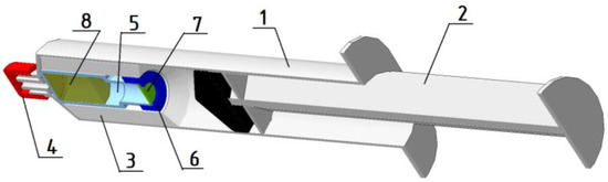
Figure 1.
Section of 3D model of the 222Rn isotope generator: 1—body (30 cm3 medical syringe); 2—syringe plunger; 3—PTFE insert; 4—sealed cap; 5—2 cm3 glass vial; 6—vial cap; 7—porous membrane; 8—cation exchanger KU-2-8 with 226Ra.
The radium form used in this work has a number of advantages over its solid salts: radium ions adsorbed on cationite are fixed on surface ionogenic groups, as a result of which the radon formed during their decay easily and with sufficient yield passes into the gas phase. This eliminates the need to work with radioactive powders, and the performance of the 222Rn generator can easily be increased by adsorption of an additional amount of 226Ra.
2.2. Experimental Facility for the Radon Dynamic Adsorption
The study of radon adsorption under dynamic conditions was carried out at an experimental research facility (Figure 2).
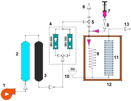
Figure 2.
Scheme of the experimental facility for studying of the radon dynamic adsorption: 1—compressor; 2—column with indicator silica gel; 3—column with activated carbon; 4—air flow control and measurement unit; 5—three-way L-shaped valve; 6—air discharge into the ventilation; 7 –222Rn input point; 8—shut-off valve; 9—metal heat exchanger; 10—overpressure meter at the entrance to the adsorption column; 11—sectioned adsorption column; 12—dry air thermostat; 13—air output from the column to the exhaust ventilation system.
During the experiment, the air from the laboratory is supplied by the compressor (1) to two columns connected in series filled with an indicator silica gel (2) and activated carbon (3), where water vapor and impurities of volatile organic compounds are removed. Volumetric air flow is regulated in unit (4), including electronic rotameters Bronkhorst MassView MV-304 (measuring range 0.04–20 l/min) and MV-302 (measuring range 0.02–2 l/min). The former was used for an air flow of up to 2 l/min or more, while the latter was used to measure and regulate lower flows. Switching between rotameters was performed by a three-way L-shaped valve. Radon was impulsively injected into the air stream from an isotopic generator connected to input point (7). Then, air flow passed through a corrugated metal heat exchanger (9), placed in a dry air thermostat (12), where it was heated to a predetermined temperature. Overpressure measurement point (10) is provided before the adsorption column inlet (11). The overpressure value was used to calculate the value of flow through the adsorbent bed, since the temperature and pressure of the gas in the adsorption column (11) differ from the standard (20 °C, 101,325 Pa). The coefficient of expansion/compression of the air flow entering the column was calculated according to Equation (1), assuming that the laws of the ideal gas were applicable:
where ke—the coefficient of expansion/contraction of the air flow in the column, Tc—column temperature, °C, Pa—atmospheric pressure, Pa, and ΔPc—overpressure in the column entrance, Pa.
The collapsible adsorption column is made of stainless steel and consists of 15 sections, with an inner diameter of 50 mm and a height of 11.5 mm each [15,16]. The bottom of the sections is a metal mesh with a cell size of 1 mm. Rubber gaskets between the sections serve to seal the entire structure. Before each experiment, 10 g of adsorbent a was poured into the column section, after which the sections were tightened with steel screws. Before radon was supplied, the column with the sorbent was thermostated for two hours at the experimental temperature (30 ± 0.1 °C) in a dry air stream with a given flow rate. Then, 222Rn was injected into the system with a short (1–2 s) pulse. The radon in the air flow was divided into sections of the sorbent column due to adsorption/desorption processes. The air pump was stopped after a set time, and the column was removed from the thermostat and disassembled. Activated carbon samples from each section were quickly poured into sealed plastic containers and thoroughly mixed with shaking.
2.3. Radiometry
222Rn itself practically does not emit γ-photons during decay (the output of γ-quants with an energy of 510 keV is only 0.076% [17]). 222Rn was measured by its daughter decay product, 214Pb:
Before measurement, the containers with the sorbent were kept for at least 5 h (the time required to establish a radioactive equilibrium between 214Pb and 222Rn). It should be noted that radon decay can lead to distortion of the results when column sections are measured for a long time. For example, if the total measurement time of all 15 sections is 10 h, radon activity in the last section will decrease by 7.3% of the original by the time it is measured. In this case, it is necessary to correct the measurement results for radon decay (to bring about the start of the measurement of the first section). The corrected value of the counting speed is calculated according to Equation (2), which also takes into account the decay of radon during the measurement of the section:
where Jc—section count rate after correction (brought to the beginning of all measurements), J—measured section count rate, J0—background count rate, λRn—decay constant of 222Rn, tm—section measurement duration, and ts—section measurement start time (counted from the beginning of all measurements).
All measurements were carried out on a Multirad-Gamma γ-spectrometer. The multichannel analyzer “Multirad Gamma” on the basis of the detector Nal(TI) registers radiant energy in the range of 60–3000 (keV) using characteristic (particular) gamma lines. The energy resolution for a line of 0.661 MeV was not more than 8.5%. The minimum measured activity (per caesium-137 count) was 3 Bq. The required duration of each measurement was calculated according to Equation (3). The relative mean square deviation of the sample count rate, due to the statistical nature of radioactive decay, did not exceed 2%. For low-activity samples (calculated tm > 1 h), the measurement time was limited to 1 h.
where ω—relative mean square deviation.
2.4. Determination of the Characteristics of the Adsorbent Bed
Activated carbon AG-3 (ENPO Neorganica JSC) was used as an adsorbent. These were dark gray cylindrical granules with a diameter of 1.5–2.2 mm and a 2.3–6.8 mm length. Bulk density (the ratio of the mass of the material to the volume it occupies, considering the space between the particles) was measured on the AUTOTAP (Quantachrome Instruments) bulk density analyzer. It was necessary to know the solid density of sorbent particles to calculate the fraction of the external free volume. That is, the ratio of their mass to the volume they occupy (including the volume of pores), without considering the free space between them. The measurement was carried out by hydrostatic weighing in ethanol of a sample saturated with molten paraffin according to the procedure described in [18,19]. The external porosity in the adsorbent bed was calculated based on the values of bulk and apparent density:
where ε—the external porosity in the sorbent bed, ρs—the solid density, g/cm3, and ρb—the bulk density, g/cm3.
For activated carbon AG-3, the solid and bulk densities were 0.449 and 0.799 g/cm3, respectively, and the external porosity in the adsorbent bed was 0.439.
3. Results and Discussion
3.1. Solution of the Inverse Problem of Radon Adsorption Dynamics
The inverse problem of adsorption dynamics is to find unknown parameters (equilibrium and kinetic) according to the experimentally obtained output curve or the measured distribution of the adsorbate concentration in the adsorbent bed. The use of output curves to solve the inverse problem of radon adsorption dynamics is described in the literature for both frontal [3,10] and elution chromatography [5,8] modes. All these approaches are based on the mathematical treatment of the experimentally obtained time dependence of the radon concentration at the outlet of the column of a known length. However, it is often difficult to accurately measure the profile of the output curve at low-volume gas activity. It seems more convenient to measure the activity of radon or its daughter nuclides in a sectioned column with a sorbent, for example, by the method of γ-spectrometry. Splitting the sorbent into layers is arbitrary, as the thickness of the layer is determined by the thickness of the column section. As a result, the inverse problem of radon adsorption dynamics can be reduced to the calculation of unknown model parameters, not by the output curve, but by the discrete distribution of activity within the column.
The effect of radioactive decay of radon on its distribution by column sections during pulse injection will be negligible as the rate of adsorption equilibrium is much higher than the decay rate of 222Rn (T1/2 = 3.8235 days [17]).
The measured radon activity in each section was divided by the total activity of all sections of the column, thus obtaining the distribution of relative activity by sections:
where An—measured activity of the column section with the number n, AEx(n)—experimental relative activity of the n-th section of the column, and N—total number of sections in a column.
On the other hand, a similar distribution of radon in sections can be obtained by integrating the function of the theoretical distribution of activity along the sorbent bed:
where h—thickness of the adsorbent bed in each section, AT(n)—theoretically calculated relative activity of the n-th section of the column, and a(x,t)—theoretical function of distribution of radon activity in the adsorbent bed.
The functions a(x,t) and AT(n) in Equation (6) implicitly depended on the Henry’s constant, the kinetic parameters of the model, and the constant parameters of the experiment (external porosity in the bed, gas linear velocity, experiment duration, etc.).
To find the parameters of the dynamic adsorption of radon, the problem of nonlinear optimization (least squares method) was solved:
where KH—Henry’s constant and Params—set of kinetic parameters of the model.
Minimization of the functional F in Equation (7) can be easily carried out using various numerical algorithms (gradient descent method, nonlinear conjugate gradient method, etc.).
The number of unknown kinetic parameters, as well as the type of function, a(x,t), in Equation (6), are determined by the theoretical model of adsorption dynamics.
We used the equilibrium adsorption layer model that contains a single kinetic parameter—the thickness of the equilibrium adsorption layer. This model is described in detail in papers by the author A.V. Larin [20,21,22,23,24]. In the column, at any given time, the thickness of the adsorbent layer (Le) can be determined, for which the condition is fulfilled: the average amount of adsorption in this layer, (ā), is the equilibrium to concentration at the outlet. Thus, at any time, t, these two quantities are related by the adsorption isotherm equation:
where x0—coordinate of the beginning of the equilibrium adsorption layer, ā(x0,t)—average value of adsorption in a layer of thickness Le with the beginning at x0 at time t, L—thickness of the equilibrium adsorption layer, a(x,t)—adsorbate concentration in the solid phase at the point with coordinate x at time t, c(x,t)—adsorptive concentration in the gas flow at the point with coordinate x at time t, and f—a function of the adsorption isotherm equation (for a linear isotherm f(c) = KH·c).
Equation (8) is carried out with any arbitrary selection of the adsorption layer beginning, x0.
To quantify the dynamics of adsorption on a column of arbitrary length, the latter is divided into k elementary layers, Le (k = L/Le, L—column length). In this case, for each i-th layer, the equation of material balance at any given time will be as follows:
where —average concentration in the mobile phase and the average adsorption in the i-th layer, ci-1(t)—adsorptive concentration at the entrance to layer i (at the exit from layer i-1) at time t, ci(t)—adsorptive concentration at the outlet of the i-th layer at time t, ε—external porosity of the column bed, u—superficial (referred to the total section of the layer) linear flow velocity, v—volumetric air flow at the column inlet, and d—inner diameter of the column.
The values of concentration and adsorption here refer to the volume of the gas and solid phases, respectively.
The solution of the system of k differential equations allows us to fully describe the distribution of the adsorbed substance in the entire column at any given time. Important advantages of the described approach are the simple numerical solution of the system for any type of adsorption isotherm, the presence of a single kinetic constant (Le) in the model, and its independence from the degree of adsorbent filling within the wide range of the concentration change (last confirmed experimentally in [23]).
In the case where the adsorption isotherm is linear, the solution of the system of material balance (Equation (9)) can be represented in analytical form [25,26]:
where c0—the adsorptive concentration at the exit from the first equilibrium adsorption layer at the initial moment of time.
The validity of Equation (11) for arbitrary (real) values of n was shown in [27] when replacing the factorial in the denominator with the Euler gamma-function through the ratio z! = Γ(z + 1). This makes it possible to calculate the concentration in the stream for an arbitrary axial x coordinate:
It should be noted that the model described above operates on the average adsorption value in each Le layer, thus being discrete with respect to the axial coordinate. However, the thickness of the discrete layers for a particular physical column is constant (determined by its design) and generally does not coincide with Le. Therefore, it is necessary to know the analytical form of the function a(x,t) to solve the inverse problem. Obviously, the real function of radon activity distribution along the adsorbent bed should be smooth. Below, we derive an analytical expression for the smooth activity distribution function of adsorbed radon in the adsorbent bed. To simplify the recording, we will, where possible, omit the second argument (time), since we are referring to the state of the column at a particular point in time.
Any layer of equilibrium adsorption (Le) can be divided into an arbitrarily large number of q sublayers, each with a thickness of ∆x = Le/q. Then, we can write the Equation (15) for the i-th layer using the mean value of the function on the segment (14), the additivity property of a definite integral, and Equation (9):
where —average adsorption value in the i-th layer, a(x)—adsorbate concentration in the solid phase at a distance x from the beginning of the column, and c(x)—adsorptive concentration in the gas flow at a distance x from the beginning of the column.
Here, we consider the case of a linear isotherm for which the kind of function, c(x,t), is given by Equation (13).
Let the column consist of Ne layers, Le, and, respectively, Ne·q sublayers of ∆x thickness. On each j-th sublayer , the function a(x) will also have an average value :
Since the choice of the origin of coordinates in the column, from which the equilibrium adsorption layers are counted, can be arbitrary, Relations (18)–(19) will be valid:
Substituting (18) into (19) gives (20):
Since , we can replace on each sublayer with the value a(x) B in its middle. Then, Equation (20) can be rewritten as follows for an arbitrary axial x coordinate:
It is obvious that the limit on the right side of Equation (21) is equivalent to the definition of the derivative of the function c(x) at point x, taken with the negative sign:
Thus, the value of the function a(x) at an arbitrary point can be expressed in terms of its value at a point shifted to the right by the value of Le, and its derivative at that point:
Using the recurrence Relation (23), one can express a(x) in terms of its value, at a point located to the right of any number, ν, of integer layers:
Since with the pulsed injection of radon into the column , we can write:
Differentiating (13) by x, we express the derivative in Equation (24) explicitly through the digamma-function Ψ:
As a result, we came to an analytical expression for calculating a(x,t) at any arbitrary point in the column at time t:
Since series (28) is convergent, to construct a smooth curve a(x,t), it is sufficient to sum according to Formula (29) until the contribution of the next term to the result becomes less than the predetermined level of the error of the calculations. At the same time, the value of the sum must be positive. The desired smooth function a(x,t) in (28) depends on the equilibrium (KH) and kinetic (Le) parameters of the model, as well as on the parameters of the experiment—the gas superficial linear velocity and the external porosity of the column bed (included in b). Numerical experiments have shown that the basic equation of the model (8) is satisfied for the function a(x,t) given by Equation (28) at arbitrary values of the parameters (KH, Le, t, u, ε). With a given value of the calculation error of 10−8%, the discrepancy between the right and left parts of Equation (8) did not exceed 10−10.
Note that in order to calculate the theoretical distribution of radon in a column according to Equation (6), we need to calculate not the function a(x,t) itself, but its definite integral. Since the antiderivative of the derivative of a function is the function itself, the definite integral a(x,t) can be expressed from (25) using the Newton–Leibniz formula as follows:
Substituting (29) and (13) into (6) gives:
The infinite series included in (30) can be expressed in terms of gamma functions as follows:
Here, Γ(x,z) is an upper incomplete gamma function.
Substituting Equation (31) into (30), we finally obtain a simple analytical expression that allows us to calculate the theoretical distribution of adsorbed radon in the column at an arbitrary point of time:
For the first section of the column, the second term in the first multiplier in (33) turns to zero. The coefficient b here includes the parameters of the model and the conditions of the experiment, and it is calculated by Equation (12).
Using Equation (33) it is possible to calculate the value of the functional (7) for any set of parameters (KH, Le). Minimizing the functional (7) will result in values of the Henry’s constant and the thickness of the equilibrium adsorption layer, allowing to best describe the experimentally obtained distribution of radon activity by column sections. This will be the solution of the inverse problem of radon adsorption dynamics.
3.2. Calculation of Radon Henry’s Constant and Thicknesses of the Equilibrium Adsorption Layer
The parameters of radon dynamic adsorption were determined on activated carbon AG-3 by an illustration of the possibilities of the developed approach. Before the experiment, the activated carbon was dried in the air stream at 170 °C for 10 h (to constant mass) to remove adsorbed water. The amount of activated carbon in each column section was 10.0 g. The volume flow of the carrier gas (dry air) was kept constant in the column (2.0 l/min). The experiment time after the pulse input of 222Rn was different. In the second series, both parameters, the air flow and the experiment time, were varied. The total volume of air passing through the column (120 l) was kept constant. For example, if the gas flow rate was cut by 4 times, the exposure time of the column was multiplied, etc.
The relative activity values of radon in columns according to Equation (5) are presented in Figure 3 and Figure 4. Each experimental data bar is provided with a confidence interval for a confidence probability of 95%. This considers the uncertainty of radiometry caused by the statistical nature of radioactive decay.
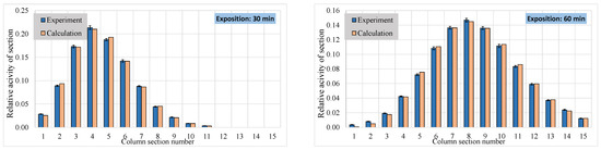
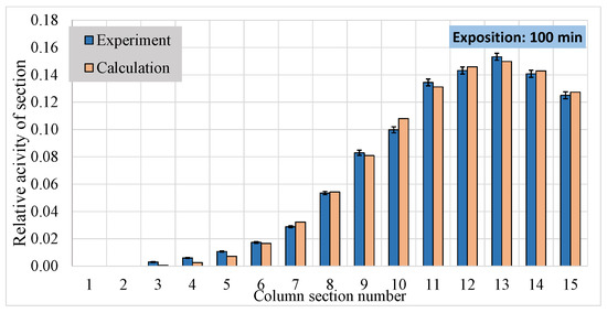
Figure 3.
Experimental and calculated distribution of 222Rn by column sections in the first series of experiments (No. 1–3 in Table 1).
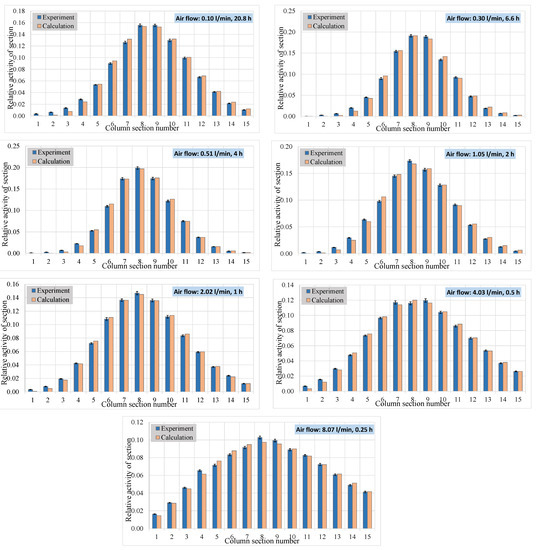
Figure 4.
Experimental and calculated distribution of 222Rn by column sections in the second series of experiments (No. 4–9 in Table 1).
These values were used to calculate the Henry’s constant and the thickness of the equilibrium adsorption layer according to Equations (7) and (33), which correspond to minimal mismatch between the calculation and experimental data. All calculations were carried out in the PTC MathCAD Prime 8 Massachusetts, USA. The theoretical (calculated) distribution of 222Rn activity into column sections was obtained using KH and Le for each experiment according to (33). The results of the comparison of calculated and experimental data are presented in Figure 3 and Figure 4. The values of parameters of dynamic radon adsorption are provided in Table 1. It also shows the standard deviation (S) of the calculation results (AT) from the experimental data (AEx).

Table 1.
Parameters of dynamic adsorption of radon on AG-3 (at 30 °C).
Henry’s constant (KH) in Equations (16)–(29) and Table 1 is a dimensionless quantity and has the physical meaning of the equilibrium concentration constant. The results of the calculation are quite well-matched and do not depend on the radon distribution by sections of the column.
The average Henry’s constants in the first and second series of experiments were 1382 ± 37 and 1336 ± 39, respectively (confidence intervals were calculated for a confidence probability of 95%). The results suggest that the volumetric velocity of the gas flow at a sufficiently wide interval does not significantly affect the results of the Henry’s constant calculation. Increased contact time of the column with the air flow after the injection of radon causes the shift of the maximum distribution of radon towards the exit of the column with simultaneous broadening (Figure 3). However, despite significant differences in the radon distribution within the column, the results of Henry’s constant in the former experiments were also close and well-correlated with the results of the latter experiments.
The parameter Le is a kinetic constant of dynamic adsorption and is close in a physical sense to the height of the equivalent theoretical plate (HETP), first proposed by the authors of the plate theory of liquid chromatography [28]. By analogy with HETP, Le is the sum of the individual terms expressing the constants of elementary kinetic stages (adsorption kinetics, longitudinal transport, etc.) [22]. Le can serve (like HETP) as an indicator of the efficiency of the sorbent bed: the smaller it is, the faster the processes of distribution of the substance between the phases proceeds and the more efficiently the adsorption column works.
Le (as opposed to Henry’s constant) depends on the gas linear velocity (see Table 1). This dependence is similar to the dependence of HETP on the gas linear velocity and is due to the same factors. Numerically, it can be expressed by the van Deemter equation, first proposed for HETP in [29]:
where A, B, and C are coefficients that consider vortex, longitudinal diffusion, and mass transfer, respectively.
Coefficients in (34) depend on the temperature, as well as the properties of the solid and mobile phases. This issue is considered in detail, for example, in [29,30].
Graphically, the dependence of Le on the air flow velocity is shown in Figure 5. The parameters A, B, and C in (34) were found using the least squares method. They were 0.353, 2.86, and 6.99 × 10⁻³, respectively.
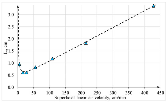
Figure 5.
Dependence of the equilibrium adsorption layer thickness on the superficial air velocity. Dots—experiment, dashed line—calculation according to Equation (33).
From Figure 5 it follows that with a decrease in the air linear velocity from 430 to 5 cm/min, the efficiency of the granular bed first increased, passed through the maximum, and then decreased. The optimal air linear velocity with the sorbent under study was about 20 cm/min. In this case, the efficiency of the granular bed was maximum (and corresponding to the minimum of Le). With a decrease in the air linear velocity to 5 cm/min, the efficiency of the column decreased due to an increase in the contribution of diffusion factors.
Using the found parameters of dynamic adsorption (Table 1), smooth curves of the radon activity distribution along the adsorbent bed were calculated for different experimental conditions, such as column exposure time and air flow rate (Figure 6 and Figure 7). The calculation was carried out for the adsorbent bed thickness of 25 cm, which exceeds the physical amount of activated carbon in the experimental column. The function a(x,t) was calculated from Equation (28) by applying an integral normalization to it:
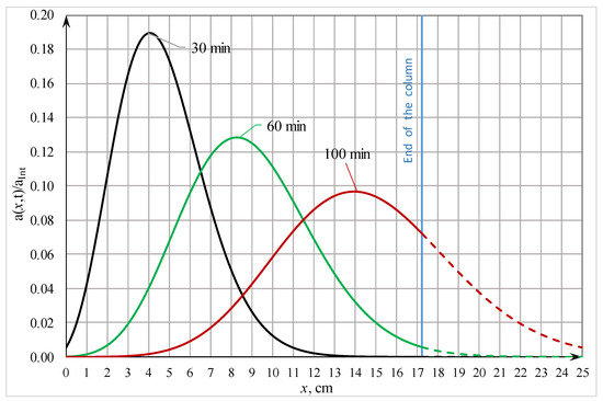
Figure 6.
Calculated distribution of 222Rn activity in the carbon bed according to the first series of experiments (No. 1–3 in Table 1).
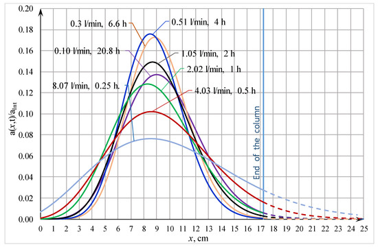
Figure 7.
Calculated distribution of 222Rn activity in the carbon bed according to the second series of experiments (No. 4–9 in Table 1).
Using relations (29) and (31), it is easy to show that aInt = KH·Le.
The dependencies of radon distribution along the adsorbent bed on the axial coordinate are close to Gaussian curves with a slight asymmetry, which increases with the displacement of curves to the ordinate axis (decrease in exposure time with constant air flow, Figure 6).
Figure 6 makes it possible to trace the evolution of the radon concentration profile in the sorbent with an increase in exposure time: as radon moved to the exit from the column, the profile of its concentration stretched along the abscissa axis, contracting simultaneously in the direction of the ordinate axis.
A series of curves in Figure 7 correspond to conditions of different efficiency of the adsorbent bed. With an increase in the air flow rate, the efficiency of the bed decreased, which led to an increase in Le and a stretching of the radon activity profile along the abscissa axis. As a result, the radon breakthrough occurred much earlier with the same total amount of air supplied to the system. A similar result was also caused by a decrease in volumetric air flow to 0.1 l/min (corresponding to a superficial gas linear velocity of 5.2 cm/min). The optimal value of air flow through the experimental column was 0.3–0.5 l/min (air superficial linear velocity, 15–30 cm/min). The profile of radon activity in the bed in this case was the narrowest. From a practical point of view, this means that the smallest amount of sorbent will be required to achieve a given degree of purification at this flow rate.
4. Conclusions
Based on the theory of the equilibrium adsorption layer, an analytical expression was obtained for calculating the smooth function of the adsorbed radon distribution in the column bed for the eluent chromatographic mode (the adsorptive is injected into the gas flow by a short pulse). The developed mathematical model was applied to the study of the dynamic adsorption of 222Rn on activated carbon in a layer-by-layer measurement of the activity of its γ-radiating daughter product (214Pb). An algorithm for calculating the Henry’s constant (KH) and the thickness of the equilibrium adsorption layer (Le) was proposed based on data of the discrete distribution of adsorbed radon over sections of a collapsible column. Two series of experiments were carried out. In each series, either the exposure test time (30 to 100 min) or the superficial linear gas velocity (5 to 430 cm/min) varied. The results showed that neither parameter had a significant influence on the calculation of Henry’s constant. The average values in the first and second series of experiments (1382 ± 37 and 1336 ± 39, respectively) were quite close.
It was shown that the kinetic adsorption parameter (Le) in a wide range of gas flow velocities (from 5 to 430 cm/min) was described by the van Deemter equation. The optimal air linear velocity with the studied sorbent was 15–30 cm/min, which meets the minimum thickness of the equilibrium adsorption layer and, accordingly, the maximum efficiency of the column bed. The developed approach is characterized by the simplicity of the experiment and can be used to study the dynamic adsorption of radon on other adsorbents or to calculate gas-cleaning equipment systems.
Author Contributions
Conceptualization, E.P.M. and A.O.M.; methodology, V.S.P. and A.V.O.; software, A.O.M.; validation, I.Y.L. and A.S.C.; resources, E.A.V.; data curation, A.O.M.; writing—original draft preparation, V.S.P. and A.V.O.; writing—review and editing, V.S.P. and A.V.O.; visualization, I.Y.L. and A.S.C.; supervision, E.P.M.; project administration, E.P.M.; funding acquisition, E.P.M. All authors have read and agreed to the published version of the manuscript.
Funding
This research received no external funding.
Data Availability Statement
Not applicable.
Conflicts of Interest
The authors declare no conflict of interest.
References
- Kiselev, S.M.; Zhukovsky, M.V.; Stamat, I.P.; Yarmoshenko, I.V. Radon: From Fundamental Research to Regulation Practice; FGBU SRC Burnasyan FMBC, FMBA of Russsia: Moscow, Russia, 2016; p. 432. [Google Scholar]
- United Nations Scientific Committee on the Effects of Atomic Radiation (UNSCEAR). Sources-to-Effects Assessment for Radon in Homes and Workplaces, Effects of Ionizing Radiation; UNSCEAR: Vienna, Austria, 2006; pp. 197–334. [Google Scholar]
- Kapitanov, Y.P.; Pavlov, I.V.; Semikin, N.P.; Serdyukova, A.S. Adsorption of radon on activated carbon. Int. Geol. Rev. 1970, 12, 873–878. [Google Scholar] [CrossRef]
- Wang, Q.; Qu, J.; Zhu, W.; Zhou, B.; Cheng, J. An Experimental Study on Radon Adsorption Ability and Microstructure of Activated Carbon. Nucl. Sci. Eng. 2011, 168, 287–292. [Google Scholar] [CrossRef]
- Pushkin, K.; Akerlof, A.; Anbajagane, D.; Armstrong, J.; Arthurs, M.; Bringewatt, J.; Lorenzon, W. Study of radon reduction in gases for rare event search experiments. Nucl. Instrum. Methods Phys. Res. A 2018, 903, 267–276. [Google Scholar] [CrossRef]
- Wang, M.; Gu, Y.; Li, F.; Ge, L.; Lu, H.; Luo, L. Study on the influence of the gas superficial velocity on the radon adsorption of activated carbon. J. Phys. Conf. Ser. 2019, 1423, 1–7. [Google Scholar] [CrossRef]
- Thomas, J.W. Evaluation of Activated Carbon Canisters for Radon Protection in Uranium Mines; Health and Safety Laboratory—United States Atomic Energy Commission (Office of Information Services, Technical Information Center): New York, NY, USA, 1974. [Google Scholar]
- Gaul, W.C.; Underhill, D.W. Dynamic adsorption of radon by activated carbon. Health Phys. 2005, 88, 371–378. [Google Scholar] [CrossRef] [PubMed]
- Yang, H.; Shan, J.; Li, J.; Jiang, S. Microwave desorption and regeneration methods for activated carbon with adsorbed radon. Adsorption 2019, 25, 173–185. [Google Scholar] [CrossRef]
- Guo, L.; Wang, Y.; Zhang, L.; Zeng, Z.; Dong, W.; Guo, Q. The temperature dependence of adsorption coefficients of 222Rn on activated charcoal: An experimental study. Appl. Radiat. Isot. 2017, 125, 185–187. [Google Scholar] [CrossRef]
- Panov, S.V.; Vlasov, A.A.; Dubovskoj, A.A.; Aristov, A.V.; Panova, O.A.; Aristova, I.A.; Panova, E.S. Radon generator with displacing gas pre-heating device. A61G 10/02 (2006.01) RU2690743C1, 5 June 2019. [Google Scholar]
- Prichard, H.M.; Mariën, K. Desorption of Radon from Activated Carbon into a Liquid Scintillator. Anal. Chem. 1983, 55, 155–157. [Google Scholar] [CrossRef]
- National standard of the Russian Federation. Iodine Sorbents for Nuclear Power Plants. Method for Determining the Sorption Capacity Index; Standartinform Publ.: Moscow, Russia, 2019. (In Russian) [Google Scholar]
- Magomedbekov, E.P.; Merkushkin, A.O.; Obruchikov, A.V.; Pokalchuk, V.S. Trapping of noble radioactive gases and their decay products under static and dynamic conditions by highly porous materials. Radioactive waste 2021, 17, 33–37. (In Russian) [Google Scholar] [CrossRef]
- Obruchikov, A.V.; Magomedbekov, E.P.; Merkushkin, A.O. The composite sorption material for radioiodine trapping from air stream and the method for its preparation. J. Radioanal. Nucl. Chem. 2020, 324, 331–338. [Google Scholar] [CrossRef]
- Obruchikov, A.V.; Merkushkin, A.O.; Magomedbekov, E.P.; Anurova, O.M. Radioiodine removal from air streams with impregnated UVIS® carbon fiber. Nucl. Eng. Technol. 2021, 53, 1717–1722. [Google Scholar] [CrossRef]
- LiveChart of Nuclides. IAEA Nuclear Data Services. 2022. Available online: https://www-nds.iaea.org/relnsd/vcharthtml/VChartHTML.html (accessed on 1 April 2022).
- Magomedbekov, E.P.; Merkushkin, A.O.; Obruchikov, A.V.; Pokalchuk, V.S. Argon, krypton and xenon adsorption coefficients on various activated carbons under dynamic conditions. J. Radioanal. Nucl. Chem. 2022, 33, 1091–1100. [Google Scholar] [CrossRef]
- Magomedbekov, E.P.; Merkushkin, A.O.; Obruchikov, A.V.; Sakharov, D.A. Comparison of the Sorption Capacity of Different Brands of Activated Carbon Relative to Argon, Krypton, and Xenon with the Natural Isotopic Composition under Static Conditions. Theor. Found. Chem. Eng. 2021, 55, 1152–1168. [Google Scholar] [CrossRef]
- Larin, A.V. Model of the equilibrium adsorption layer in chromatography. Communication 1. Statement of the problem and general mechanisms of nonideal chromatography for different sorption isotherms. Bull. Acad. Sci. USSR Div. Chem. Sci. 1984, 33, 1112–1115. [Google Scholar] [CrossRef]
- Larin, A.V. Application of the model of the layer of equilibrium adsorption to non-ideal non-linear chromatography. J. Chromatogr. A 1987, 388, 81–90. [Google Scholar] [CrossRef]
- Larin, A.V. Layer-by-layer method in adsorption dynamics. I. New variant of the method, initial equation, and the possibility of a numerical solution. Bull. Acad. Sci. USSR Div. Chem. Sci. 1983, 32, 1114–1118. [Google Scholar] [CrossRef]
- Larin, A.V. Layer-by-layer method in dynamics of adsorption. Communication 2. Solution of reverse problem. Bull. Acad. Sci. USSR Div. Chem. Sci. 1983, 32, 2391–2395. [Google Scholar] [CrossRef]
- Larin, A.V. Solution of the inverse problem and calculation of sorption isotherms in chromatography. J. Chromatogr. A 1986, 364, 87–95. [Google Scholar] [CrossRef]
- Larin, A.V. On the correct measurement of retention and Henry constant on short adsorbent layer. Prot. Met. Phys. Chem. Surf. 2011, 47, 743–747. [Google Scholar] [CrossRef]
- Larin, A.V. On calculation of the effectiveness of a low-length adsorbent layer. Prot. Met. Phys. Chem. Surf. 2013, 49, 642–645. [Google Scholar] [CrossRef]
- Larin, A.V. Elution on adsorbent beds of short length. Analytical solution. Russ. Chem. Bull. 2011, 60, 376. [Google Scholar] [CrossRef]
- Martin, A.J.P.; Synge, R.L.M. A new form of chromatogram employing two liquid phases. Biochem. J. 1941, 35, 1358–1368. [Google Scholar] [CrossRef]
- van Deemter, J.J.; Zuiderweg, F.J.; Klinkenberg, A. Longitudinal diffusion and resistance to mass transfer as causes of nonideality in chromatography. Chem. Eng. Sci. 1956, 5, 271–289. [Google Scholar] [CrossRef]
- Gritti, F.; Guiochon, G. The van Deemter equation: Assumptions, limits, and adjustment to modern high performance liquid chromatography. J. Chromatogr. A 2013, 1302, 1–13. [Google Scholar] [CrossRef] [PubMed]


Publisher’s Note: MDPI stays neutral with regard to jurisdictional claims in published maps and institutional affiliations. |
© 2022 by the authors. Licensee MDPI, Basel, Switzerland. This article is an open access article distributed under the terms and conditions of the Creative Commons Attribution (CC BY) license (https://creativecommons.org/licenses/by/4.0/).