1. Introduction
1.1. Background
Excessive noise emissions of hydraulic pumps are a known drawback of hydraulic control technology, which has limited its application or acceptance in various fields that involve human operators in proximity to a hydraulic system. This technology limitation has motivated the hydraulic fluid power community toward the development of solutions for noise mitigation, such as resonators or silencers. An extensive summary of the devices created during the last decade can be found in [
1]. An even higher effort has been put toward the ideation of design principles for pumps capable of reducing noise generation. As a result, several low noise solutions for the most popular pump designs (such as axial piston pumps and gear pumps) have been conceived. Focusing on the case of external gear pumps (EGPs), which is also the pump design considered in this study, in the literature it is possible to find several fundamental studies related to the principles of fluid-borne noise generation, as well as designs specifically conceived for so-called “low noise” pumps. In the first category of studies, particularly relevant are the works by Molton [
2] and Manring [
3], which assess the kinematic flow ripple on EGPs and provide criteria for reducing it by acting on the tooth profile. Borghi et al. [
4] also addressed the effects of the timing of the internal connections of the tooth space volumes, which also influence the fluid-borne noise. As described in [
5], a proper design of the internal porting connections can improve the noise generation of an EGP. Recently, Zhao and Vacca [
6] presented a generalized method to model the fluid-borne noise of EGPs through a simple lumped parameter approach.
The area of low-noise EGPs is widely populated in the literature and supported by several designs of commercial success. The most widely adopted low-noise pump solution consists of the dual-flank principle, first introduced by Negrini [
7], which is based on involute gears operating with zero backlash. Other design concepts that improve the noise emission of standard involute gear pumps are based on helical designs [
8,
9]. Unconventional tooth profiles were also recently commercialized specifically to reduce the kinematic flow ripple. Among these, the continuous contact design principle [
10,
11] and the asymmetric tooth profile design [
12,
13] are those that already found successful commercial applications.
Despite their effectiveness in reducing noise and vibration, the above-mentioned approaches and design solutions focus on minimizing the fluid-borne noise (FBN) source, which is frequently represented by outlet flow/pressure ripple, without taking a structural path into account or quantifying the radiated noise level. This can be a limitation in the context of further pushing the technology toward solutions capable of further reducing noise emissions. Particularly for EGPs, the need for quieter solutions has become more stringent in recent years as a consequence of the recent electrification trend affecting the market of mobile applications. In a conventional diesel-powered vehicle, the presence of the combustion engine has helped in masking the noise generated by the hydraulic system. When replacing the diesel engine with an electric prime mover, the noise and vibration by hydraulic pumps become instead a primary issue. Furthermore, the speed regulation flexibility of electric motors has allowed more widespread use of EGPs, which are fixed displacements, to replace the more expensive variable displacement piston pumps.
Therefore, there is a current need for a deeper understanding of the structure dynamic behaviors of EGP to further advance low noise technology. Moreover, the development of an accurate and computationally inexpensive numerical modal model is the first crucial step in developing an effective virtual prototyping tool for addressing the noise aspect during the design stage. In this light, this paper experimentally and numerically investigates the modal behaviors of hydraulic pumps with the reference of EGPs.
1.2. State of the Art
The available literature on experimental modal analysis (EMA) of positive displacement machines addresses different aspects. Most studies have conducted EMA as an intermediate step to validate structural models, which are parts of the numerical vibroacoustic models for the prediction of noise and vibration responses during machine operation [
14,
15,
16,
17,
18]. EMA has also been used to investigate the resonant behaviors of the system, to explore the contribution of noise sources to the structure- and air-borne noise [
19], or to achieve noise reduction by avoiding the coincidence between the excitation and resonant frequencies [
20]. To fulfill their objectives, these past studies show how important it is to identify the modal frequencies of the pump. However, the mode shapes of the pump body have been mostly overlooked and not thoroughly studied.
With respect to the subject of numerical modal analysis of hydraulic pumps, many past studies have employed finite element methods (FEM). There can be multiple sources of modeling uncertainties and difficulties in FE structural dynamics, which have been extensively discussed by Ibrahim [
21]. Among many of these challenges, the current study focuses on three aspects arising from the nature of the pump components assembly and mounting uncertainties of: (1) material properties of each component; (2) bolted joints; and (3) boundary conditions. The following paragraphs of this section discuss how these uncertainties were handled in previous studies, including fields other than pump analysis.
Few studies have addressed the uncertainties of material properties by using numerical modal analysis. Relevant examples are the works by Kouroussis [
22] and Tabatabaei [
23], who utilized FE modal analysis in comparison with experimentally measured modal parameters to estimate realistic material properties of timber beams and functionally-graded materials. However, except for one study by Xu [
17], this topic has not been often discussed in the existing hydraulic noise and vibration studies. Because hydraulic units are formed by several components, overlooking this aspect may serve as a non-negligible source of model inaccuracies.
Another important aspect related to the assembly of multiple components is the modeling of the bolted joints, as they introduce some complicated contacts at the interfaces between components [
21]. Opperwall and Schleihs utilized the bonded contact between the elements [
18,
24], which is the simplest way to account for the bolted connections, but this approach can result in large inaccuracies, as it usually introduces a larger stiffness than the actual one. Instead, Mucchi [
15], Xu [
17], and Pan [
25] presented more advanced models in which the bolt shank and thread parts are modeled as beam elements and the connections between bolt heads and neighboring elements are modeled with interpolation spiders. However, these works do not clarify how to treat the contact interface between bodies realized by bolted connections. On the contact due to the bolted joints, Fiebig [
20] briefly mentioned considering the presence of frictional contact at the interface in his modal model of a fluid power unit, although no modeling details were presented.
Lastly, the definition of the boundary conditions associated with pump mounting is not straightforward. A common practice that can be found in many existing studies is using idealized constraints, such as fixed boundary conditions [
16,
26,
27,
28]. However, this simple assumption of considering fixed boundary conditions can lead to large errors in the FE model, as discussed in [
29].
1.3. Limitation of Past Work
Past work on experimental modal analysis of hydraulic pumps lacks an investigation of the vibration mode shape characteristics. The understanding of the behavior of these mode shapes is crucial since they serve as the basis of vibration fields during operation. The vibration modes are often used to transform the governing equation from physical spaces into modal coordinates. After solving the equation in modal coordinates, the vibration field responses are obtained by transforming the modal solutions back to physical space, which is known as the modal superposition method [
30]. In modal superposition, the calculation of the modal response heavily depends on the interaction between the spatial distributions of the loads and mode shapes. During pump operation, however, the dynamic loads generated by the working fluid in physical space occur in a distributed manner from many different coherent sources, rather than a simple force acting on a point or a few points [
31]. Therefore, without a clear understanding of mode shapes, it is difficult to comprehend how the vibration field responds to distributed loads. Furthermore, depending on the mode shapes, each structural vibration mode has a different noise radiation efficiency and directivity pattern [
32]. As a consequence, it is also important for understanding the pump noise radiation characteristics and conducting noise control.
With respect to the numerical modal analysis of hydraulic pumps, the previous subsection highlights how three modeling challenges (uncertainties of material properties, bolted joints, and boundary conditions) are handled in the existing studies. The limitations of each aspect can be summarized by the following points.
The lack of consideration for uncertain material properties in most existing numerical analyses of hydraulic pumps implies that it is an easily overlooked topic. This is probably because the basic material properties of components, such as steel and cast iron, are usually well known. However, in practice, the actual material properties of each component may have differences, and this can lead to errors that stack up when multiple components are assembled.
Regarding bolted joints, previous studies used different modeling approaches with various levels of complication. Some of them were oversimplified. For advanced methodologies, on the other hand, what remains unclear is how to treat the contact interfaces between bodies realized by bolted connections. Using the FE model and leaving them untreated can result in possible penetration issues between bodies, which is clearly unrealistic.
Concerning the modeling boundary conditions, it is common practice to use an idealized fixed boundary condition. However, there is no such material that can provide a perfectly rigid structural foundation, so the parts assigned with the fixed constraints can still move, and this must be accounted for in order to increase model accuracy [
21,
29].
1.4. Research Objectives
The main goal of this research is to provide a methodology to perform a modal analysis for EGPs following both an experimental and numerical modal analysis approach. This main goal is accomplished by pursuing the following objectives on a specific EGP:
To experimentally characterize and categorize the modal behaviors of the pump, reflecting the specific mounting of the test rig used in this research, with an emphasis on the mode shape features.
To determine the mode shapes through vibration measurements and advanced post-processing. Although the modal parameter extraction theory is well established, the actual implementation usually requires some user interactions [
30], which is scarcely addressed in the hydraulic field. Therefore, some practical aspects of the modal parameter extraction technique that can be used for this purpose will be presented as well.
To propose a modeling methodology that addresses the challenges of uncertainties of material properties, bolted joints, and boundary conditions with minimal model complexity. The objective of the proposed model is to achieve good accuracy with minimal computational load, so that the model can be used in the future for design considerations and virtual prototyping.
By achieving the above-mentioned objectives, the proposed experimental and modeling approaches also aim to contribute to similar noise and vibration research of other types of hydraulic pumps because they address common aspects that other units have, although a single EGP is analyzed in this paper.
1.5. Structure of the Paper
This paper is structured as follows. The external gear pump taken as reference and the test apparatus including the pump mounting is introduced in
Section 2. The experimental modal analysis is discussed in
Section 3 from the experimental setup through the modal parameter extraction techniques and the main results. The numerical modeling strategies for modal analysis using FEM, as well as the validation against the modal parameters obtained with EMA, will be given in
Section 4.
2. Reference Unit and System
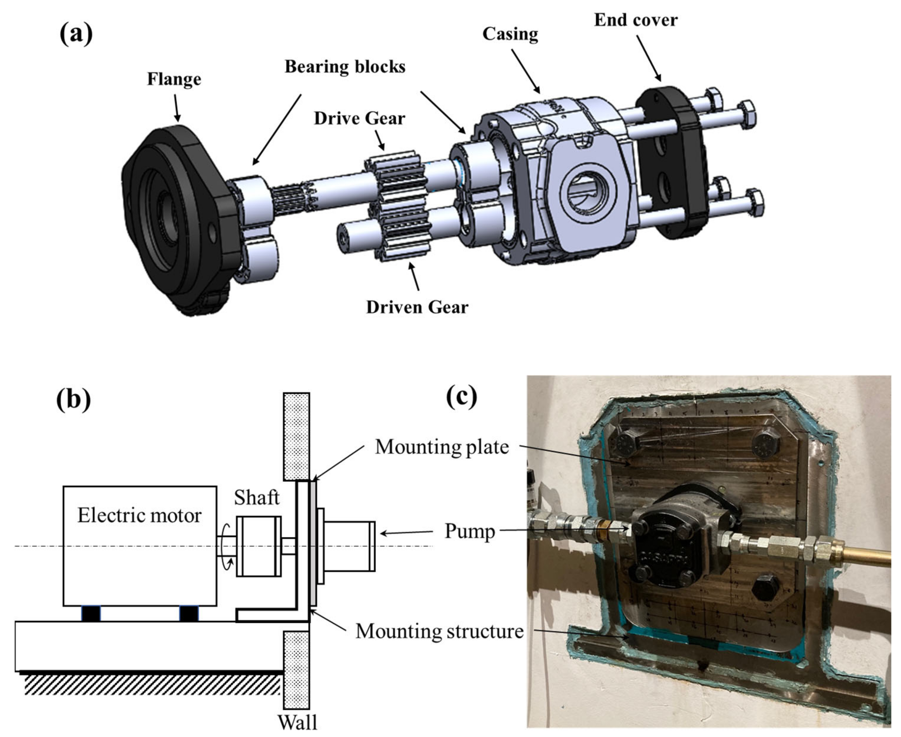
Figure 1a shows the exploded view of the reference external gear pump (Casappa model PHP20). Three exterior parts, the flange, casing, and end cover, form the complete housing connected by the four bolts. The inlet and outlet ports are located at each side of the casing. Inside the casing are two bearing blocks and a pair of standard involute spur gears (drive and driven gears), whose number of gear teeth is 12. The nominal displacement of the unit is 22 cc/rev, and it uses pressure-compensated lateral balancing mechanisms. The unit is for moderate- and high-pressure applications, which can be operated up to 250 bar for constant operation with a maximum speed of 3500 rpm.
The operating principle of EGPs, in brief, can be explained starting by defining the volumes enclosed by casing and gears as the tooth space volume (TSV). The flow enters from the inlet port due to the expansion of TSVs as the gear teeth move out of the meshing zone. The trapped fluid in the TSVs then travels around the casing toward the outlet. Finally, flow is discharged to the output port due to the contraction of the TSVs in the meshing region. A more detailed description of the working principle of EGPs can be found in [
33].
Figure 1b,c illustrates how the reference unit is mounted to the test rig—the semi-anechoic chamber at the authors’ lab, the Maha Fluid Power Research Center of Purdue University. Any hydraulic pump must be connected to a prime mover, in this case an electric motor, and couplings and fixtures are needed for this connection accommodating misalignment. In this study, the connection between them is realized with a mounting plate along with a mounting structure, along with the spline couplings for the shaft, as shown in the figure.
Of all these components, the modal behaviors of the pump body are of primary interest. However, those of the mounting plate are examined as well since prior research done by the authors has shown that the mounting has a great contribution to the radiated noise during the operation of the pump [
34,
35].
3. Experimental Modal Analysis
This section provides an overview of the experimental modal analysis (EMA) procedure and the results performed with the reference EGP mounted to the test rig. To better understand the vibration characteristics of the system, the experimental work is presented here first, followed by a discussion of the numerical modeling in
Section 4. This work uses an impact test, which is a frequently used approach for EMA, to extract modal parameters, such as modal frequencies, mode shapes, and modal damping. The main results will be provided at the end of the section after covering some practical aspects of experimental procedures and modal parameter extraction techniques.
3.1. Test Setup
Figure 2 shows the impact test setup for EMA. An impact hammer is used to excite the system and measure the impulsive force signal applied to the system. For a given excitation, the responses in terms of acceleration are measured using three triaxial accelerometers. The acceleration and force signals were acquired using a National Instruments data acquisition system with the software LabVIEW. The list of equipment and their specifications are provided in
Table 1.
3.2. Frequency Response Function (FRF)
The frequency response function (FRF) is a fundamental measurement used to extract modal parameters of the system. FRF is a transfer function of how much response the system has per unit excitation in the frequency domain [
30]. In this case, the excitation is the impulsive force measured with the impact hammer, and the response is the acceleration measured with accelerometers. The post-processing procedures to obtain FRFs from the measured force and acceleration signals are briefly discussed in the following paragraphs.
Once the force signal is measured, the force window is applied to the signal. This is because, after the impact, there is no excitation anymore to the system while the electrical noise will still be measured in the force signal. The force window removes this electric noise after the impact, allowing for clearer FRF. For a similar reason, the exponential window is applied to the acceleration signals to minimize the deterioration of the signal from the noise after the response has decayed from the system damping. After applying the corresponding windows to both signals, the power spectral density (PSD,
) and cross-spectral density (CSD,
) are estimated based on Welch’s method. Here, subscript
represents the response (acceleration) signal while
represents the excitation (force) signal. From these PSD and CSD, the FRF is finally calculated using the
estimation method since the
estimator is robust to the contamination of the response signal by noise.
More details about this procedure can be found in [
36].
There are three types of FRFs depending on what kind of response signal is used, namely receptance, mobility, and inertance. The FRF determined with the displacement is called the receptance. Likewise, if velocity and acceleration are used, the FRFs are called mobility and inertance, respectively. Although the measured signals with accelerometers are accelerations, the FRFs with acceleration (inertance) are converted into the receptance by taking integrals with respect to time twice because most of the modal parameter extraction theories are usually derived with the receptance. Thus, it should be noted that in this document, all measured FRFs represent the receptance unless otherwise mentioned.
Figure 3a presents the points of the measurements on the pump and mounting plate, and
Figure 3b shows all the measured FRFs in terms of the receptance at 52 points using triaxial accelerometers (52 points × 3 directions = 156 degrees of freedom) with the excitation at point 1. Some modal frequencies can be identified from the simple observations of the peak locations in the FRFs, but the estimation of modal damping ratios and modal vectors requires more advanced post-processing. Thus, the following sections discuss how the modal parameters are extracted from these FRFs.
3.3. Modal Parameter Extraction
As the name suggests, modal parameter extraction (also widely known as modal parameter estimation) is a method to extract modal information from a single FRF or a set of FRFs. In essence, the main idea is to curve-fit the mathematical expressions with the unknown modal parameters to the measured FRFs or the impulse responses. Many methods have been developed for modal parameter extraction from the FRF, such as the peak-picking (PP) method, circle-fit (CF) method, rational fraction polynomial (RFP) method, least-square complex exponential (LSCE) method, and Ibrahim time-domain (ITD) method [
30]. Among these methods, in the current study, the LSCE method is selected considering the adequacy of application to the system and the extent of complexity of implementation. For the implementation in this study, the built-in functions for LSCE provided by the MATLAB toolbox (System Identification Toolbox) are used.
3.3.1. Determination of the Model Order Using a Stabilization Diagram
One practical difficulty when applying most of the modal parameter extraction methods for the multi-degree of freedom system is the determination of the model order, indicating how many modes should appear in the measured FRFs. It would be straightforward if the system were simple and lightly damped, such that the peaks at the resonant frequencies were clearly visible in the measured FRFs. Then, one could simply count the number of peaks in the frequency range of interest and use it for the model order. For many cases, however, the measured FRFs may not display distinct and clear peaks when the structure is complex, having many parts with bolted joints and/or highly damped. Therefore, a more effective way to determine the model order is needed. Several methods have been developed to overcome this difficulty, but one of the most widely used methods is a stabilization diagram [
30]. The idea is to check the behaviors of the modal frequencies and damping factors with increasing model order. As the model order increases, the curve-fitting algorithm (LSCE in this study) identifies a greater number of modal frequencies. These identified modes can consist of two types of modes. One is the real (physical) modes, and the other is the ‘computational’ modes, which are numerically introduced to have the optimum curve fit to minimize the error. As the model order gets larger, the poles of the real modes remain substantially the same while those of the computational modes change. Using this fact, a stabilization diagram can be generated.
Figure 4 shows the stabilization diagram obtained from the measured FRFs at low-frequency regions. The red curve represents the magnitude of the FRF averaged with the FRFs of all degrees of freedom. The ordinate on the left side in blue shows the model order, and the blue dots with three different symbols (
) represent the modal frequencies determined by the poles with the corresponding model orders. The symbol is chosen according to specific criteria as follows. As mentioned before, if there are the physical poles among the poles with the model order
, then the values of the physical poles almost do not change, determined with the model order
. In this regard, the poles that do not change much as compared to the consecutive model order increase are considered “stable”. Note that the real part of these poles is related to the damping ratios, while the imaginary part is associated with the modal frequencies (
). Thus, how much change of the modal frequencies and damping ratios exhibit as compared to the next model order are the criteria to determine if the poles are stable. These criteria are set with the 1% change for the modal frequency and the 5% change for the damping ratio. The reason for the higher value of the criterion (meaning the loose criterion) for the damping ratio is that the damping ratios are more sensitive to the change of the model order. If both criteria are satisfied, the cross symbol (+) is used in the plot to indicate the stable poles. If the criterion for the modal frequency is met but not with the damping ratio criterion, the circle symbol (o) is used to indicate the partially stable poles. Lastly, if both criteria are not satisfied or the determined poles do not have the complex conjugate pair (
), the unstable poles are indicated with the dot symbol (
). As can be seen in the figure, the stable and partially stable poles form the straight vertical lines around the peaks of the averaged FRF graph. According to this plot, for the reference case, the model order is selected with 9. This procedure is repeated with a reasonable selection of the frequency interval up to 5 kHz.
Although the stabilization plot aids in determining model order, it is still not determined whether the choice provides reliable results. To check if the chosen model order is reasonable, the FRF at each point is compared. Once the modal parameters are determined, the corresponding FRF can be regenerated, and this regenerated FRF is then compared with the measured FRF. As an example,
Figure 5 shows the comparison between the measured FRFs (blue line) and the regenerated FRFs (red line) at one point on the plate (left) and another point on the pump (right). It is shown that both magnitude and phase of FRFs have a good agreement, which implies that the choice of the model order is satisfactory. In case of a mismatch, another choice can be made for the model order based on the stabilization diagram above, and the whole procedure can be repeated until reasonable results are achieved.
3.3.2. Decision on the Acceptance or Rejection of the Identified Modes
The previous part illustrated the model order selection. Even if this results from the stabilization diagrams and the regenerated FRF agrees well with the measured FRF, this does not necessarily imply that all of the identified poles are “good” poles corresponding to physical modes. The computational poles may still be included among the recognized poles, as discussed in
Section 3.3.1. Furthermore, although certain poles may be derived from physical modes, if they are not sufficiently excited (e.g., vertical bending modes excited with force in the horizontal direction), their reliability may be compromised owing to the poor signal-to-noise ratio at those modal frequencies. In this light, it is still necessary to choose which modes, among the detected poles, should be preserved or discarded. This was accomplished in this study by evaluating the mode shapes using the following logic.
Let us take an example of the identified poles obtained in the previous subsection. As shown in
Figure 6, the modal vectors corresponding to the identified poles may be displayed in the complex plane, and two modal vectors are provided in the figure for reference. Each dot in three distinct colors indicates the modal vector component in the x, y, and z directions. Technically, the mode shape should be real-valued, which means that all of the dots in the complex plane plot should be on the abscissa. However, because the measured FRFs are not exactly in line with the mathematical formulation, the modal vector obtained with the LSCE algorithm still outputs an imaginary component in the real measurement. To assess how close the modal vector components are to the real-valued, the regression line (illustrated by the green line in the figure) for each vector is generated based on total least squares in the complex plane. For a modal vector
of the length
, the slope (
) of the line can be obtained by using the singular value decomposition (SVD):
where
,
,
are
,
,
matrices that constitute the singular value decompositions, and
and
are (1,2) and (2,2) elements of the matrix
. The details of the total least squares can be found in [
37]. If the modal vector is physical, the slope of the green line should be close to zero, and most of the points sit on the line, as can be seen on the left side of the figure. This means that the real parts are far greater than the imaginary parts, so they are close to the real-valued. In this case, the mode is accepted. On the other hand, if the identified modal vector is not physical or obtained from “poor” measurement, such as the ones with a low signal-to-noise ratio, the points in the plane are usually scattered and the slope of the regression line is large, as shown on the right side of the figure. Therefore, this mode is rejected. In this study, the acceptance criterion is the absolute value of the slope angle being less than 15°, which was determined heuristically based on the observation from the measured data. These procedures are repeated for multiple intervals of the frequency range up to 5 kHz.
3.4. Experimental Modal Analysis Results
Table 2 summarizes the modal frequencies and damping ratios of the 38 modes identified up to 5 kHz, and
Figure 7 depicts the experimental mode shapes. For the sake of brevity, only the significant mode shapes are reported in the figure. The mode shapes are categorized based on the type of motions that the modes exhibit—vertical and horizontal binding, longitudinal, and torsional motions of the pump. The mode shapes that exhibit the far larger plate motions compared to the pump motions are also shown at the bottom of the figure, and they are referred to as the plate motion dominant modes. Some key observations can be made at this point. At low frequencies below 1 kHz, the vertical and horizontal bending motions are mainly observed. The modes in the frequency range from 1 to 2 kHz are mostly the modes with the dominant plate motions. Starting from 2 kHz, many torsional modes show up until around 4 kHz. As the frequency increases, many other modes with plate-dominant motions are observed again, and their deflections show higher spatial variations.
3.5. Discussion on Vibration Reduction Strategies during Pump Operation
Another important thing to note about the mode shapes is that the pump casing itself does not show any significant deformation up to 5 kHz. Instead, its motion is close to the rigid body motion. It has a significant implication that can aid in the development of vibration reduction strategies from the source level. According to previous research by authors [
35], the vibration field responses that the external gear pump exhibits during operation are similar to the superposition of the vibration modes observed in this study. This observation suggests that the overall structural vibrations can be reduced by suppressing the modal responses, which are proportional to the modal forces. The modal forces of each mode are obtained by taking the inner products between mode shapes and dynamic loads in space. However, there are multiple coherent sources of the dynamic loadings in external gear pumps occurring in a distributed manner during an operation inside the casing [
31]. If the mode shapes of the pump casing have large spatial variations as well, it is only after calculating the modal forces that it is possible to predict if design changes would lower modal responses. In this case, without taking the structural model into account, the simple reduction of the magnitudes of noise sources may not work well for vibration reduction. On the other hand, for a given mode whose mode shape is close to the rigid body motion, the modal force will be proportional to the net forces and moments acting on the mass center of the casing obtained with the distributed loads in physical space. As evaluating net forces and moments is relatively straightforward, it will enable the development of more intuitive vibration reduction solutions from the source level because the interaction between the distributed loads and mode shapes does not have to be considered.
4. Numerical Modal Analysis
This section addresses key challenges related to the development of numerical modal analysis tools for hydraulic pumps, according to what was also mentioned in the introduction:
Material properties. Even small errors in material properties for each component can bring to larger stack-up errors when the components are assembled.
Bolted joints. Oversimplifications of bolted joints in the model can lead to large errors, while advanced modeling methods usually involve nonlinear contacts and high computation costs.
Boundary conditions at constraints. Assuming simplistic boundary conditions to model the constraints, such as fixed boundary conditions, usually leads to large errors depending on the situation. This is because no material can provide a perfectly rigid structural base, so that the parts where the fixed boundary conditions are assigned can actually move.
In this regard, this section discusses how these three aspects are addressed in the model to capture the dynamic behaviors determined with the experimental modal analysis.
4.1. Modal Analysis of Each Component to Estimate Material Properties
The first step to achieving a realistic numerical modal model is to carefully determine the material properties without simply considering generic values provided by general sources. The real material properties may differ from these values. It would be ideal to access measurements of material properties taken from the tests of specimens of each element, although this is often impractical and it requires specialized test equipment. Therefore, in this study, the material properties are estimated by performing a numerical and experimental modal analysis of each component in a free boundary condition.
The material properties required for the structural dynamic analysis are density (), Young’s modulus (), and Poisson’s ratio (). Among them, the density is the simplest to measure; for each component, the weights can be measured with a scale, and the volumes are calculated from the CAD file. Then, the density is obtained by dividing the measured weight by the volume. Unlike the measurement of density, there is no simple and practical way to measure Young’s modulus and Poisson’s ratio without special equipment and sensors, such as tensile testing machines and strain gauges. Thus, in the free boundary condition, each element is tested with the impact test and two material properties are tuned in the numerical analysis until they have good agreement in terms of both the modal frequency and modal vectors.
Figure 8 shows the setup of the experimental modal analysis for each component with an example of the mounting plate. As shown in the picture, each component is hung up on the rack by the elastic rubber band, which is the common practice to realize the free boundary condition. Then, the impact test and post-processing are carried out with the same procedure described in
Section 3. After having the experimental results, Young’s modulus and Poisson’s ratio are manually estimated to minimize the error in corresponding modal frequencies.
Table 3 presents the comparison of numerical modal frequencies with the experimental modal frequencies obtained with the initial and estimated values of the material properties of the mounting plate. When initial values are used (default material properties provided by ANSYS,
,
,
), the numerical modal frequencies are underpredicted with a maximum error of 3.47%. Although it shows reasonable agreement, the small error may stack up when simulating the assembly of the pump with the mounting structure, so it can be a good practice to minimize the error at a component level. After using the estimated values of the material properties (
,
,
), the error in the modal frequencies could be reduced smaller than 0.25%. Moreover,
Figure 9 shows a comparison of experimental and numerical mode shapes. The modal assurance criterion (MAC) values are reported together in the figure to quantify the agreements between the modes. The MAC between two mode shape vectors
and
is defined as [
30,
38,
39]:
The MAC values range from zero to unity, with the two vectors with the high correlation having a value close to one. In this regard, the comparisons between the numerical and experimental mode shapes show reasonable agreement, with MAC values greater than 0.8. Although only the result with the mounting plate is presented here for brevity and confidentiality, the same procedure was followed for all other components in the system.
4.2. Modeling of Assembled Parts with Bolted Joints
The way the mechanical connections between the assembled parts are treated in the numerical model highly affects its results. The system under study makes significant use of bolted joints, and for this reason, these are the type of mechanical connections taken into consideration in this work. The simplest way to model the bolted joints is to bond the whole interface between the elements, which makes them act like a single body. For some simple systems, this method can provide reasonably accurate results. However, as will be demonstrated in this subsection, this simple assumption can lead to non-negligible errors for the reference case. Therefore, this study proposes a simple way to model bolted connections that provides reasonable accuracy without requiring a significant modeling effort.
Figure 10a shows the normal stress distribution when the clamping force is applied to the bolt for the connections of two elements, and it is the normal stress that holds two pieces together. The normal stress decreases as the distance from the bolt increases and eventually goes to zero [
40]. From this fact, it is assumed that the regions where the normal stress exist are glued to each other, as shown in
Figure 10b. Usually, this region looks like a conical frustum, and the angle made by the bolt head and the radius of this region is defined as the pressure angle (
). The pressure angle normally ranges between 25° and 33° [
41], and bonding the area of interfaces where normal stress exists is a common way to model bolted joints. However, what remains uncertain is how to treat the area of interface outside of this region. Without any treatment to the area outside of the merged region, there is a penetration issue, as there is no mechanical element to stop the movement of elements going toward each other in that region. There have been few past works discussing this penetration issue; in particular, a way to prevent the penetration aspect has been suggested by Yoo et al. [
42]. They introduced an array of springs to the area outside of the merged area, and the number and stiffness of the springs were determined by the design of the experiment (DOE) method. Based on this idea, a simpler alternative method is proposed in this study. In ANSYS software, when frictionless contact is applied to the contact region, it will put the springs between the contact area, as shown on the right side of
Figure 10c and the spring constants will be determined by the augmented Lagrange method [
43].
Figure 10d shows one mode shape of the pump without contact condition (left) and with frictionless contact (right). It shows that the penetration issue is resolved after the frictionless contact is applied, but still allows the sliding motion between parts.
The proposed method for modeling bolted connections using the merged conical frustum along with the frictionless contact is applied to the full assembly of the mounting plate and pump, and it is tested with the free boundary condition, as shown in
Figure 11. Starting with a typical value of 30°, the pressure angle for bonding at each interface is adjusted until it provides good agreement with the experimental results. To assess the improvement achieved with the proposed method, the numerical simulation is also done with the bonded contacts applied to all the interfaces.
Table 4 summarizes the comparison between experimental and numerical modal analysis results for the full assembly of the mounting plate and the pump in the free boundary condition. Note that the mode is listed with the ascending order of the experimental modal frequencies, and corresponding numerical modes after comparing the mode shapes are reported accordingly in the table. When the bonded contacts are applied to the whole interface between all the elements, the modal frequency shows a significant difference from the measurement. The simulation overpredicts the modal frequency due to the increased stiffness as the whole interfaces are assumed bonded while they are not. It can also be seen that the mode order differs from the measurement; the numerical modal frequency corresponding to the first experimental mode is greater than the one corresponding to the second experimental mode. However, after considering the bolted connections, the numerical mode orders are in the same order as the measurement. Furthermore, it shows a good agreement of both modal frequencies, as well as mode shapes, as shown in
Figure 12.
In summary, the proposed approach to simulate bolted connections is easy to implement and does not significantly increase the model complexity, and it is simpler compared to the more advanced model of existing studies using beam element and spider interpolation by Xu and Pan [
17,
25]. Although it is not directly comparable, the test configuration is similar to the one used by these authors in that the hydraulic pump assembly was tested in a free boundary condition. The achieved accuracy in their study is with the maximum error of 3.3% (average error of 1.0%) and 4.31% (average error of 1.67%), respectively. Considering that the maximum error in this study is 5.6% with an average error of 1.73%, it can be concluded that the proposed approach still provides comparable accuracy to the advanced one.
4.3. Numerical Modal Analysis Results
This subsection illustrates the most complete results of the numerical modal analysis, which mimics the scenario of the pump mounted to the test rig structure. The section also compares the simulation results with the experimental modal analysis. Before presenting the results, how the boundary condition is treated in the numerical model will be discussed.
Figure 13 shows the numerical and experimental modal analysis setup for the pump installed on the test rig. The assembly of the mounting plate and the pump in
Section 4.2 is mounted to the mounting structure via four bolted joints. For these connections, the same approach discussed in the previous subsection is used in the numerical model.
Figure 14 illustrates the assigned boundary condition for the bolted connections of the mounting structure. In fact, the mounting structure is connected through the bolted joints to the elastic base of the electric motor (see
Figure 1). Thus, to obtain a realistic model for the system, all of the components indicated in
Figure 1b, such as the base, electric motor, shaft couplings, and torque meter, should be incorporated in the model. However, this would require extensive modeling and significant computational resources, which is not necessary since their dynamic behaviors are not of interest in this study. Therefore, to simplify this aspect, the other structures are first assumed to be rigid. Then, to model the connections between the mounting structure and the rigid base, a similar approach of modeling bolted connections can be used; the conical frustum region may be created for the four bolt holes where the structures are connected. With this assumption, the easiest boundary condition that may be assigned is a fixed boundary condition at the frustrum area. However, as will be shown in the results, it results in a considerable discrepancy as compared to the experimental results due to the high stiffness. For the convenience of presenting results, this boundary condition is indicated as “fixed support”. To remedy the issue, instead, for those frustum areas, the elastic support boundary condition is assigned with the large foundation stiffness in the normal direction while the tangential directions are fixed (represented in purple in the figure) to imitate the bonded contact with the elastic body. For the area outside of the conical frustum area, the elastic support boundary condition in the normal direction with smaller foundation stiffness (represented in green in the figure) and no boundary conditions in tangential directions are assigned to imitate the frictionless boundary condition. This proposed boundary condition will be referred to as “elastic support”. These foundation stiffnesses for the elastic support boundary condition are properly calibrated to match the experimental results.
Table 5 presents the comparison between numerical and experimental modal frequencies of the first six modes. Note that the mode order here is based on the order of numerical modal frequencies of the elastic support case, and corresponding modes are identified by observing the mode shapes. When the results of the fixed support case are compared to the experimental results, the mode orders differ, and large discrepancies in the modal frequencies are observed up to 85% (average 37.1%). Moreover, the fact that most of the numerical modal frequencies are greater than the experimental ones implies that the fixed boundary conditions make the system stiffer than it is. The use of elastic supports can alleviate this problem; after updating the boundary conditions with the elastic support, the numerical and experimental results show reasonable agreement with an accuracy of less than 11% error (average 6%). Furthermore, the numerical results follow the same model order as the experimental results. Lastly,
Figure 15 compares the numerical and experimental mode shapes and shows good agreement between them.
5. Conclusions
This study presents a method for studying the dynamic characteristics of an external gear pump (EGP) considering their actual mounting, following both a numerical and an experimental approach for modal analysis.
An impact test is employed in the experimental modal analysis. Up to 5 kHz, a total of 38 modes have been identified, with the following characteristics. When it comes to modal damping, the majority of the modes have a relatively high damping ratio, greater than 1% and up to around 4%. Furthermore, the mode shapes are categorized depending on the type of motions that the modes exhibit—vertical and horizontal bending, longitudinal, and torsional motions of the pump, as well as the plate motion dominant modes. One thing to note about the mode shapes is that the pump casing itself does not show any substantial deformation but is close to the rigid body motion, whereas the mounting plate shows higher-order deformations. From this observation, it was discussed that the vibration reduction strategies can be developed in a straightforward manner; it implies that source level reduction (minimizing the net forces and moments acting on the mass center of the casing) during pump operation can be effective even if the structural model is not involved.
In the numerical modal analysis, three aspects are primarily considered in this work: (1) estimate of material properties; (2) bolted joint modeling; and (3) boundary conditions modeling. First, the material properties are estimated using values that provide the least amount of modal frequency error when compared to those obtained by experimental modal analysis of each component. Second, the proposed method for modeling bolted joints is tested with the full assembly of the mounting plate and the pump in free boundary conditions. In comparison to the case where the whole interfaces are bonded, the proposed approach provides better agreements with a significant reduction in maximum errors from 46.4% (average 20.8%) to 5.6% (average 1.73%). When compared to the advanced approach of bolted connections in the existing studies with higher modeling complexities, this approach still provides comparable accuracy. Finally, the case where the pump mounted to the test rig is modeled and tested. As the mounting structure is linked to the elastic base, assigning fixed boundary conditions (fixed support case) gives rise to large stiffness, resulting in significant errors in modal frequencies of up to 85% (average 37.1%). To relieve the strong constraints, the boundary conditions with the elastic support are proposed (elastic support case), and the maximum error could be decreased to 10.8% (average 6%).
As a final remark, it should be acknowledged that the novelty of this work lies in the way existing modeling approaches are combined for the first time to provide an effective method to address the main research goal. Moreover, the proposed experimental and modeling approaches can be applied to other types of hydraulic pumps as well. In this regard, this paper may serve as a guideline for modal analysis of hydraulic pumps.
Author Contributions
Conceptualization, S.W. and A.V.; methodology, S.W. and A.V.; software, S.W.; validation, S.W. and A.V.; formal analysis, S.W. and A.V.; investigation, S.W. and A.V.; resources, A.V.; data curation, S.W.; writing—original draft preparation, S.W.; writing—review and editing, S.W. and A.V.; visualization, S.W.; supervision, A.V.; project administration, A.V.; funding acquisition, A.V. All authors have read and agreed to the published version of the manuscript.
Funding
This research received no external funding.
Institutional Review Board Statement
Not applicable.
Informed Consent Statement
Not applicable.
Data Availability Statement
Not applicable.
Acknowledgments
The authors would like to thank Manuel Rigosi and Antonio Lettini of the R&D department of Casappa S.p.A., Italy, for providing the physical units and technical information.
Conflicts of Interest
The authors declare no conflict of interest.
Nomenclature
| Symbols | Description | Units |
| Acceleration signal | |
| Young’s modulus | |
| Frequency | |
| Force signal | |
| Power spectral density of an acceleration signal | |
| Cross spectral density between an acceleration signal and a force signal | |
| Power spectral density of a force signal | |
| frequency response function estimator | |
| Value of modal assurance criteria | - |
| Model order for modal parameter extraction | - |
| , , | matrices that constitute singular value decompositions | - |
| element of the matrix | - |
| Pressure angle (half-apex angle of cone shape stress field due to bolted joints) | ° |
| Slope of a regression line | - |
| Pole of -th mode () | |
| Damping ratio of -th mode | - |
| Poisson’s ratio | - |
| , | Mode shape vector | - |
| Density | |
| Modal frequency of -th mode | |
| Superscripts | Description | |
| Hermitian | |
| Complex conjugate | |
| Acronyms | Description | |
| CSD | Cross spectral density | |
| DOE | Design of experiment | |
| EGP | External gear pump | |
| EMA | Experimental modal analysis | |
| FBN | Fluid-borne noise | |
| FEM | Finite element method | |
| FRF | Frequency response function | |
| LSCE | Least-square complex exponential | |
| MAC | Modal assurance criterion | |
| PSD | Power spectral density | |
| SVD | Singular value decomposition | |
| TSV | Tooth space volume | |
References
- Danes, L.; Vacca, A. A frequency domain-based study for fluid-borne noise reduction in hydraulic system with simple passive elements. Int. J. Hydromechatron. 2021, 4, 203. [Google Scholar] [CrossRef]
- Molton, G.R. Techniques for reducing fluid borne noise from gear pumps and their circuits. SAE Tech. Pap. 1987, 96, 844–851. [Google Scholar] [CrossRef]
- Manring, N.D.; Kasaragadda, S.B. The theoretical flow ripple of an external gear pump. J. Dyn. Syst. Meas. Control 2003, 125, 396. [Google Scholar] [CrossRef]
- Borghi, M.; Paltrinieri, F.; Milani, M.; Zardin, B. The influence of cavitation and areation on gear pumps and motors meshing volumes pressures. In Proceedings of the American Society of Mechanical Engineers, The Fluid Power and Systems Technology Division, FPST, Chicago, IL, USA, 5–10 November 2006; American Society of Mechanical Engineers (ASME): New York, NY, USA, 2006; pp. 47–56. [Google Scholar]
- Devendran, R.S.; Vacca, A. Optimal design of gear pumps for exhaust gas aftertreatment applications. Simul. Model. Pract. Theory 2013, 38, 1–19. [Google Scholar] [CrossRef]
- Zhao, X.; Vacca, A. Theoretical investigation into the ripple source of external gear pumps. Energies 2019, 12, 535. [Google Scholar] [CrossRef] [Green Version]
- Negrini, S. A gear pump designed for noise abatement and flow ripple reduction. Proc. Int. Fluid Power Expo. Tech. Conf. 1996, 47, 23–25. [Google Scholar]
- Huang, K.J.; Chen, C.C.; Rd, W. Kinematic displacement optimization of external helical gear pumps. Chung Hua J. Sci. Eng. 2008, 6, 23–28. [Google Scholar]
- Ransegnola, T.; Zhao, X.; Vacca, A. A comparison of helical and spur external gear machines for fluid power applications: Design and optimization. Mech. Mach. Theory 2019, 142, 103604. [Google Scholar] [CrossRef]
- Zhao, X.; Vacca, A. Analysis of continuous-contact helical gear pumps through numerical modeling and experimental validation. Mech. Syst. Signal Process. 2018, 109, 352–378. [Google Scholar] [CrossRef]
- Zhao, X.; Vacca, A. Multi-domain simulation and dynamic analysis of the 3D loading and micromotion of continuous-contact helical gear pumps. Mech. Syst. Signal Process. 2022, 163, 108116. [Google Scholar] [CrossRef]
- Morselli, M.A. Rotating Machine Tool and Process for Cutting Gearwheels with Asymmetrical Teeth 2018. U.S. Patent Application No. 15/767776, 4 October 2018. [Google Scholar]
- Devendran, R.S.; Vacca, A. Design potentials of external gear machines with asymmetric tooth profile. In Proceedings of the ASME/BATH 2013 Symposium on Fluid Power and Motion Control, FPMC 2013, Sarasota, FL, USA, 8–11 October 2013; American Society of Mechanical Engineers: New York, NY, USA, 2013. [Google Scholar]
- Zhang, J.; Xia, S.; Ye, S.; Xu, B.; Zhu, S.; Xiang, J.; Tang, H. Experimental investigation on the sharpness reduction of an axial piston pump with reinforced shell. Appl. Acoust. 2018, 142, 36–43. [Google Scholar] [CrossRef]
- Mucchi, E.; Rivola, A.; Dalpiaz, G. Modelling dynamic behaviour and noise generation in gear pumps: Procedure and validation. Appl. Acoust. 2014, 77, 99–111. [Google Scholar] [CrossRef]
- Carletti, E.; Miccoli, G.; Pedrielli, F.; Parise, G. Vibroacoustic measurements and simulations applied to external gear pumps. An integrated simplified approach. Arch. Acoust. 2016, 41, 285–296. [Google Scholar] [CrossRef] [Green Version]
- Xu, B.; Ye, S.; Zhang, J. Numerical and experimental studies on housing optimization for noise reduction of an axial piston pump. Appl. Acoust. 2016, 110, 43–52. [Google Scholar] [CrossRef]
- Schleihs, C.; Murrenhoff, H. Modal analysis simulation and validation of a hydraulic motor. In Proceedings of the 9th JFPS International Symposium on Fluid Power, Matsue, Japan, 28–31 October 2014. [Google Scholar]
- Bonanno, A.; Pedrielli, F. A study on the structureborne noise of hydraulic gear pumps. Proc. JFPS Int. Symp. Fluid Power 2008, 2008, 641–646. [Google Scholar] [CrossRef]
- Fiebig, W.; Wrobel, J. System approach in noise reduction in fluid power units. In Proceedings of the BATH/ASME 2018 Symposium on Fluid Power and Motion Control, Bath, UK, 16–19 October 2018. [Google Scholar] [CrossRef]
- Ibrahim, R.A.; Pettit, C.L. Uncertainties and dynamic problems of bolted joints and other fasteners. J. Sound Vib. 2005, 279, 857–936. [Google Scholar] [CrossRef]
- Kouroussis, G.; Ben Fekih, L.; Descamps, T. Using experimental modal analysis to assess the behaviour of timber elements. Mech. Ind. 2017, 18. [Google Scholar] [CrossRef] [Green Version]
- Tabatabaei, S.J.S.; Fattahi, A.M. A finite element method for modal analysis of FGM plates. Mech. Based Des. Struct. Mach. 2020. [Google Scholar] [CrossRef]
- Opperwall, T.; Vacca, A. A combined FEM/BEM model and experimental investigation into the effects of fluid-borne noise sources on the air-borne noise generated by hydraulic pumps and motors. Proc. Inst. Mech. Eng. Part C J. Mech. Eng. Sci. 2014, 228, 457–471. [Google Scholar] [CrossRef]
- Pan, Y.; Li, Y.; Huang, M.; Liao, Y.; Liang, D. Noise source identification and transmission path optimisation for noise reduction of an axial piston pump. Appl. Acoust. 2018, 130, 283–292. [Google Scholar] [CrossRef]
- Rodionov, L.; Makaryants, G. Simulation of Gear Pump Noise Generation. In Proceedings of the 9th FPNI Ph.D. Symposium on Fluid Power, Florianópolis, Brazil, 26–28 October 2016; pp. 1–9. [Google Scholar]
- Schleihs, C.; Murrenhoff, H. Acoustical simulation of a hydraulic swash plate motor. In Proceedings of the ASME/BATH 2015 Symposium on Fluid Power and Motion Control, FPMC 2015, Chicago, IL, USA, 12–14 October 2015. [Google Scholar]
- Milind, T.R.; Mitra, M. A study on the flexible multibody dynamic modeling of an axial piston pump considering housing flexibility. Procedia Eng. 2016, 144, 1234–1241. [Google Scholar] [CrossRef] [Green Version]
- Shi, Z.; Hong, Y.; Yang, S. Updating boundary conditions for bridge structures using modal parameters. Eng. Struct. 2019, 196, 109346. [Google Scholar] [CrossRef]
- Ewins, D.J. Modal Testing: Theory, Practice and Application; John Wiley & Sons: West Sussex, UK, 2009; ISBN 0863802184. [Google Scholar]
- Woo, S.; Opperwall, T.; Vacca, A.; Rigosi, M. Modeling noise sources and propagation in external gear pumps. Energies 2017, 10, 1068. [Google Scholar] [CrossRef] [Green Version]
- Fahy, F.J.; Paolo, G. Sound and Structural Vibration; Elsevier: Oxford, UK, 2007; ISBN 9780081020739. [Google Scholar]
- Ivantysyn, J.; Ivantysynova, M. Hydrostatic Pumps and Motors: Principles, Design, Performance, Modelling, Analysis, Control and Testing; Tech Books International Pvt. Ltd.: Maharashtra, India, 2003. [Google Scholar]
- Woo, S.; Vacca, A.; Rigosi, M. A model based approach for the evaluation of noise emissions in external gear pumps. In Proceedings of the 11th International Fluid Power Conference (IFK), Aachen, Germany, 19–21 March 2018. [Google Scholar]
- Woo, S.; Vacca, A. Experimental Characterization and Evaluation of the Vibroacoustic Field of Hydraulic Pumps: The Case of an External Gear Pump. Energies 2020, 13, 6639. [Google Scholar] [CrossRef]
- Brandt, A. Noise and Vibration Analysis: Signal Analysis and Experimental Procedures; John Wiley & Sons: West Sussex, UK, 2011; ISBN 9780470746448. [Google Scholar]
- Van Huffel, S.; Vandewalle, J. The Total Least Squares Problem: Computational Aspects and Analysis; Society for Industrial and Applied Mathematics: Philadelphia, PA, USA, 1991. [Google Scholar]
- Allemang, R.J. The modal assurance criterion-Twenty years of use and abuse. Sound Vib. 2003, 37, 14–21. [Google Scholar]
- Pastor, M.; Binda, M.; Hararik, T. Modal Assurance Criterion. Procedia Eng. 2012, 48, 543–548. [Google Scholar] [CrossRef]
- Mikid, B.B. Areas of contact and pressure distribution in bolted joints. J. Manuf. Sci. Eng. Trans. ASME 1972, 94, 864–870. [Google Scholar] [CrossRef] [Green Version]
- Kim, J.; Yoon, J.-C.; Kang, B.-S. Finite element analysis and modeling of structure with bolted joints. Appl. Math. Model. 2007, 31, 895–911. [Google Scholar] [CrossRef]
- Yoo, J.; Hong, S.-J.; Choi, J.S.; Kang, Y.J. Design guide of bolt locations for bolted-joint plates considering dynamic characteristics. Proc. Inst. Mech. Eng. Part C J. Mech. Eng. Sci. 2009, 223, 363–375. [Google Scholar] [CrossRef]
- Kohnke, P. Theory Reference for the Mechanical APDL and Mechanical Applications; ANSYS, Inc.: Philadelphia, PA, USA, 2009. [Google Scholar]
Figure 1.
(a) Exploded view of the reference external gear pump, (b) schematic, and (c) picture of the reference unit mounted to the test rig.
Figure 1.
(a) Exploded view of the reference external gear pump, (b) schematic, and (c) picture of the reference unit mounted to the test rig.
Figure 2.
Test setup of experimental modal analysis.
Figure 2.
Test setup of experimental modal analysis.
Figure 3.
(a) Measurement points and (b) all measured FRFs with excitation at point 1.
Figure 3.
(a) Measurement points and (b) all measured FRFs with excitation at point 1.
Figure 4.
The stabilization diagram obtained with the measured FRFs.
Figure 4.
The stabilization diagram obtained with the measured FRFs.
Figure 5.
Comparison between the measured FRFs (blue line) and the regenerated FRFs based on the modal parameters (red line).
Figure 5.
Comparison between the measured FRFs (blue line) and the regenerated FRFs based on the modal parameters (red line).
Figure 6.
Modal vectors are represented in the complex plane to decide whether to accept or reject the modes.
Figure 6.
Modal vectors are represented in the complex plane to decide whether to accept or reject the modes.
Figure 7.
Experimental mode shapes.
Figure 7.
Experimental mode shapes.
Figure 8.
The setup of the experimental modal analysis for each component in free boundary conditions.
Figure 8.
The setup of the experimental modal analysis for each component in free boundary conditions.
Figure 9.
Comparison between experimental mode shapes and numerical mode shapes obtained with the estimated values of material properties.
Figure 9.
Comparison between experimental mode shapes and numerical mode shapes obtained with the estimated values of material properties.
Figure 10.
(
a) Qualitative illustrations of normal stress distribution when the clamping force is applied [
40], (
b) schematic of modeling bolted connection, (
c) graphical representation for the model in FEM when contact condition is not applied (
left) and frictionless contact is applied (
right) [
43], and (
d) the mode shape of the pump when contact condition to the area outside of the merged area for the bolted connections is not applied (
left) and frictionless contact is applied (
right).
Figure 11.
Numerical and experimental modal analysis setup for the assembly of the mounting plate and pump.
Figure 11.
Numerical and experimental modal analysis setup for the assembly of the mounting plate and pump.
Figure 12.
Comparison between experimental mode shapes and numerical mode shapes of the full assembly of the mounting plate and the pump after consideration of the bolted connections.
Figure 12.
Comparison between experimental mode shapes and numerical mode shapes of the full assembly of the mounting plate and the pump after consideration of the bolted connections.
Figure 13.
Numerical and experimental modal analysis setup for the pump mounted in the sound chamber.
Figure 13.
Numerical and experimental modal analysis setup for the pump mounted in the sound chamber.
Figure 14.
Illustrative representation of the assigned boundary condition for the bolted connections of the mounting structure.
Figure 14.
Illustrative representation of the assigned boundary condition for the bolted connections of the mounting structure.
Figure 15.
Comparison of numerical (elastic support case) and experimental mode shapes when the pump is mounted.
Figure 15.
Comparison of numerical (elastic support case) and experimental mode shapes when the pump is mounted.
Table 1.
List of equipment for the impact test.
Table 1.
List of equipment for the impact test.
| No. | Description | Details |
|---|
| 1 | Impact hammer | PCB model 086D05, sensitivity: 0.23 mV/N,
measurement range: ±22,240 N |
| 2 | Accelerometer | PCB model 356A16, sensitivity: 100 mV/g
measurement range: ±50 g,
frequency range: 0.5 Hz to 5 kHz |
| 3 | Data acquisition system | National Instrument, cDAQ-9178 with NI 9234 modules, maximum sampling rate: 51.2 kS/s,
24-bit resolution, ±5 V input |
Table 2.
The experimental modal frequencies and damping ratio.
Table 2.
The experimental modal frequencies and damping ratio.
| Mode # | Frequency (Hz) | Damping | Mode # | Frequency (Hz) | Damping |
|---|
| 1 | 159.9 | 2.86% | 20 | 1370.4 | 1.68% |
| 2 | 225.7 | 3.76% | 21 | 1414.9 | 1.28% |
| 3 | 255.7 | 2.72% | 22 | 1562.4 | 1.93% |
| 4 | 288.1 | 3.98% | 23 | 1777.5 | 1.16% |
| 5 | 333.5 | 2.45% | 24 | 2210.5 | 1.34% |
| 6 | 459.9 | 3.08% | 25 | 2343.6 | 0.57% |
| 7 | 531.3 | 2.83% | 26 | 2488.5 | 0.87% |
| 8 | 643.7 | 2.40% | 27 | 2569.7 | 0.42% |
| 9 | 722.6 | 2.90% | 28 | 2747.5 | 0.92% |
| 10 | 758.0 | 1.21% | 29 | 2877.3 | 1.53% |
| 11 | 809.5 | 1.25% | 30 | 3005.4 | 1.75% |
| 12 | 826.3 | 1.59% | 31 | 3129.4 | 1.43% |
| 13 | 895.2 | 2.22% | 32 | 3499.6 | 2.05% |
| 14 | 936.6 | 1.48% | 33 | 3636.1 | 1.49% |
| 15 | 946.8 | 1.79% | 34 | 4046.5 | 0.25% |
| 16 | 1069.3 | 1.21% | 35 | 4164.1 | 1.74% |
| 17 | 1131.1 | 0.49% | 36 | 4334.0 | 1.08% |
| 18 | 1195.5 | 1.15% | 37 | 4743.6 | 0.71% |
| 19 | 1298.2 | 2.55% | 38 | 4869.6 | 2.49% |
Table 3.
Comparison of numerical modal frequencies obtained with initial and estimated values of the material properties with the experimental modal frequencies of the mounting plate.
Table 3.
Comparison of numerical modal frequencies obtained with initial and estimated values of the material properties with the experimental modal frequencies of the mounting plate.
| | Experimental | Numerical
(Initial Values of Material Properties) | Numerical
(Estimated Values of Material Properties) |
|---|
| Frequency (Hz) | Frequency (Hz) | Error (%) | Frequency (Hz) | Error (%) |
|---|
| 1 | 568.2 | 566.3 | 0.34 | 569.1 | 0.16 |
| 2 | 748.1 | 722.1 | 3.47 | 747.4 | 0.09 |
| 3 | 1022.3 | 1019.7 | 0.25 | 1020.2 | 0.21 |
| 4 | 1427.8 | 1393.1 | 2.43 | 1431.4 | 0.25 |
| 5 | 1434.4 | 1394.6 | 2.77 | 1433.0 | 0.10 |
Table 4.
Comparison of numerical modal frequencies with the experimental modal frequencies before and after the consideration of the bolted connections. The tested object is the full assembly of the mounting plate and the pump.
Table 4.
Comparison of numerical modal frequencies with the experimental modal frequencies before and after the consideration of the bolted connections. The tested object is the full assembly of the mounting plate and the pump.
| | Experimental | Numerical—Fully Bonded | Numerical—Bolted Connections |
|---|
| Frequency (Hz) | Frequency (Hz) | Error (%) | Frequency (Hz) | Error (%) |
|---|
| 1 | 650.0 | 951.6 | 46.4% | 651.0 | 0.2% |
| 2 | 699.8 | 811.5 | 16.0% | 702.9 | 0.4% |
| 3 | 812.6 | 1056.3 | 30.0% | 858.0 | 5.6% |
| 4 | 981.7 | 1133.4 | 15.5% | 996.7 | 1.5% |
| 5 | 1097.7 | 1190.4 | 8.4% | 1077.0 | −1.9% |
| 6 | 1518.7 | 1642.6 | 8.2% | 1506.4 | −0.8% |
Table 5.
Comparison of numerical modal frequencies with the experimental modal frequencies when the pump is mounted.
Table 5.
Comparison of numerical modal frequencies with the experimental modal frequencies when the pump is mounted.
| | Experimental | Numerical—Fixed Support | Numerical—Elastic Support |
|---|
| Frequency (Hz) | Frequency (Hz) | Error (%) | Frequency (Hz) | Error (%) |
|---|
| 1 | 225.7 | 373.4 | 65.5 | 250.1 | 10.8 |
| 2 | 333.5 | 617.0 | 85.0 | 319.4 | −4.2 |
| 3 | 459.9 | 463.0 | 0.7 | 410.7 | −10.7 |
| 4 | 531.3 | 700.7 | 31.9 | 517.9 | −2.5 |
| 5 | 643.7 | 621.4 | −3.5 | 593.2 | −7.8 |
| 6 | 722.6 | 982.3 | 35.9 | 723.0 | 0.1 |
| Publisher’s Note: MDPI stays neutral with regard to jurisdictional claims in published maps and institutional affiliations. |
© 2022 by the authors. Licensee MDPI, Basel, Switzerland. This article is an open access article distributed under the terms and conditions of the Creative Commons Attribution (CC BY) license (https://creativecommons.org/licenses/by/4.0/).


