Abstract
The high importance of demand-side management for the stability of future smart grids came into focus years ago and is today undisputed among a wide spectrum of energy market participants, and within the research community. The increasing development of communication infrastructure, in tandem with the rising transparency of power grids, supports the efforts for deploying demand-side management applications. While it is then accepted that demand-side management will yield positive contributions, it remains challenging to identify, communicate, and access available flexibility to the flexibility managers. The knowledge about the system potential is essential to determine impacts of control and adjustment signals, and employ temporarily required demand-side flexibility to ensure power grid stability. The aim of this article is to introduce a methodology to determine and communicate local flexibility potential of end-user energy systems to flexibility managers for short-term access. The presented approach achieves a reliable calculation of flexibility, a standardized data aggregation, and a secure communication. With integration into an existing system architecture, the general applicability is outlined with a use case scenario for one end-user energy system. The approach yields a transparent short-term flexibility potential within the flexibility operator system.
1. Introduction
Throughout the last decade, with the increasing share of renewable energy sources (RES), the demand side of the energy economy has come into focus in the research and industry activities [1,2,3,4,5,6,7,8,9]. Whereas, hitherto, the production of energy was the main measure used to strike a balance between generation and consumption, as of recently, the demand side—and its inherent flexibility—has come into focus to strike that very balance [10]. The orientation of fulfilling high energy demands in times of low RES production leads to high conventional reserves or storage capacities. These high reserve facilities lead to high costs for energy infrastructure operators and, thus, high costs for society. Additional challenges related to power quality or the location of RES are outlined in [11]. The integration of the rising share of electric vehicles (EVs) as time- and location-independent loads and potential storage devices adds an additional challenge to the energy infrastructure. Demand-side management (DSM) offers a measure to achieve a balance between generation and consumption with a reduced need for additional financial and commodity investments in the energy generation and distribution infrastructure. Whereas the importance of DSM programs is widely understood, the flexibility calculation and accessibility, such as load deviation between currents, and possible power consumption, especially when concentrating on residential areas, is still a field of activity. The challenges can be summarized by the term uncertainty. When focusing on real-time applications, different aspects contribute to uncertainty. These aspects occur through forecast errors of production facility or load states. Additional aspects are the changing user behaviour and ambient conditions that influence the device operations [1].
This work establishes a methodology as a power management system (PMS) extension that calculates a short-term reliable flexibility potential out of in-time operation conditions and end-user inputs to reduce uncertainty in local flexibility calculations. For a specific discrete time step, i Equation (1) shows the feasible power consumption of a system, expressible as the deviation between maximum and minimum power consumption. With the knowledge about the current power consumption, the accessible system flexibility for DSM measures is identifiable. Due to short-term parameter states and end-user inputs into PMS interfaces for specific smart devices, the flexibility, up to a time window of several hours, can be calculated accurately and communicated to interested entities within the wide area network (WAN). Those entities can utilize the communicated flexibility for short-term reactions to forecast deficiencies and surpluses in renewable power production or system load. Another utilization domain is short-term trading at the European Energy Exchange (EEX) or at future flexibility markets. The needed communication connections into end-user energy systems, both commercial and private, necessitate high requirements in data security and integrity, because of information that can be extracted and the insights into individual behaviour. To reduce the threats for compromising and counterfeiting, DSM measures need to be implemented into highly secure and standardised software as well as hardware architectures [12,13]. Whereas the research in flexibility is advancing, research on how to implement these into secure communication architectures to ensure the trust of end-users into DSM measures has been on the sidelines. In contrast to the very detailed communication of end-user information, generalized models of the aggregated behaviour of the system do not reflect the accurate and accessible flexibility potential [14,15]. Thus, the aggregator perspective varies from detailed end-user information to generalized system information. Putting the aggregator perspective into consideration, a new categorization of flexibility communication can be developed, which shows the improvement in the described method. The presented method combines the detailed local calculation and the abstracted aggregation to the flexibility operator through an abstraction layer. The contribution of this article is therefore summarized as follows:
- Introduction of a new categorization of flexibility studies, focusing on aggregator perspective.
- Development of an end-user oriented PMS-input interface with detailed parameters under strict comfort considerations.
- New method for a reliable flexibility calculation and data-parsimonious communication as real-time application.
- Approach to enable self-determined participation of a wide set of end-users on flexibility markets through aggregator entities.
- Integration of an abstraction layer for consideration of privacy and data security.
The structure of this article is organized as follows: in Section 2, a categorization of recent flexibility research work is performed to outline the relevance of the developed method in contrast to previous work. Additionally, the possible utilization of flexibility is shown. Section 3 describes the methodology, considering specific end-user devices. Section 4 contains the explanation on the use cases and the results of the performed simulations. In Section 5, the findings are discussed and debated. In addition, the outlook for future work is presented.
2. Flexibility Studies Overview
Insights into flexibility potential of the demand-side for integrating RES or new appliances, considering end-user behaviour, is a highly relevant research topic in literature [1,2,3,4,5,6,7,8,9,10,11,12,13,14,15,16,17,18,19,20]. Whereas different works deal with the impact or potential of DSM on aggregated [15] or individual demand [19], others try to differentiate end-users, considering their ability to contribute to pre-defined DSM mechanisms [14,20]. The latter often evaluate historical or statistical data for the clustering [9,14]. The existence of an entity that directly controls or indirectly influences the connected energy system is the main similarity in the majority of research items. The goals of the control efforts often deal with successful RES integration, system cost, or peak-to-average ratio reduction. Whereas many works focus on the above-mentioned research questions, only a few discuss categorization methodologies of flexibility and demand response (DR) studies to establish comparability, and a wider understanding of the aggregator perspective into the connected energy system. The following section develops a categorization to achieve this change of perspective.
2.1. Categorization of Flexibility Studies
Besides the categorization in this article, other possibilities were developed with their own specific purposes. Reference [3] differentiates into DR-based and DR-independent flexibility studies. DR-based approaches are tightly linked to the DSM mechanism in the research scope. The main objective is the modeling of an end-user’s responsiveness to the pre-defined DSM mechanism, realized as DR or dynamic pricing program. In contrast, DR-independent approaches model the end-user’s flexibility potential in a generalized manner. These models can be used to evaluate the impact of different DSM mechanisms on the power demand of end-user systems. Developing a new DR-independent model by evaluating open-source data for household appliances [3] presents a methodology for modeling end-user behaviour focused on white goods, here, for washing machines, tumble dryers, and dishwashers.
An additional categorization of recent flexibility studies was developed by [4]. Four patterns for the communication and exploitation of flexibility are shown. The four patterns are (a) physical demand response, (b) direct market demand response, (c) indirect market demand response, and (d) decentralized market demand response. Categories (a) and (b) gather approaches for direct load control, which send signals for individual devices or whole systems. Pattern (c) focuses on power consumption adjustments by variable tariffs. Pattern (d) is about local coordination of end-users without a central coordination entity.
When participating in today’s flexibility markets, such as reserve capacity markets or intra-day trading platforms for energy, a central coordination entity is required. The aggregation of end-users is an indispensable prerequisite, because the trading volume is limited to minimal power and duration offers. However, how the aggregator reliably and timely receives or generates flexibility potential estimations is still a matter of concern. Focusing on the aggregator perspective as a market access enabler for residential or small commercial end-users, a new categorization of flexibility studies can be developed, which embodies one contribution of this work.
2.2. Abstraction Level of Communication to Aggregator Backend
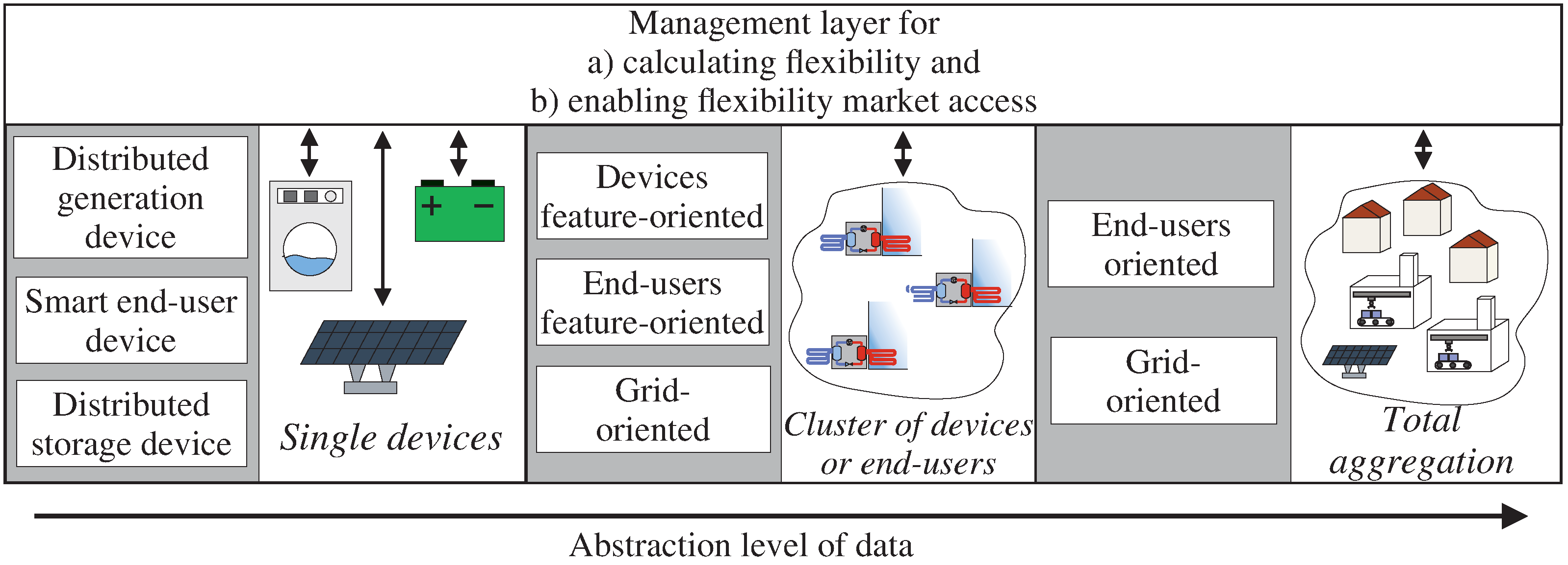
Figure 1 shows the proposed categorization by the abstraction level of the communication of flexibility or flexibility linked parameters to the aggregator backend system, and from this to the aggregated system of end-users. Distinctions can be drawn between:
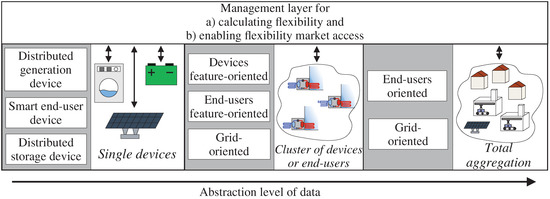
Figure 1.
Categorization of flexibility studies.
- Single Devices;
- Clusters of devices or end-users; and
- Total aggregation.
With the single devices approaches, detailed information about a specific appliance is monitored and sent directly to the aggregator backend. Through the evaluation of device or end-user features clusters of devices or end-users are generated to achieve a reduction in complexity and an increase in reliability when focusing on behaviour and reactions within the clusters. The focus on small grid areas as clusters is also possible within this categorization approach. Within the total aggregation approaches, whole distribution grids or all aggregator-connected end-users are abstracted to one entity. The categorization that is applied to the analysed works can be found in Table 1.

Table 1.
Abstraction level of communication and referenced literature.
A single devices-centred approach for modeling end-user behaviour in the area of white goods is presented in [3]. There, flexibility is broken down into three parameters, (a) deferrable energy, (b) the time of availability, and (c) the deadline to exploit the offered flexibility for individual households. Another single devices method was developed by [5], showcasing the predictive and agile balancing of a virtual power plant consisting of devices modeled as buckets, bakeries, and batteries, which reflect specific system behaviour of the applied devices. By a centralized evaluation of the individual parameters, the system’s agile balancing capabilities prioritize the operations. The main findings are a lower power consumption and short computation times. In [6], a new strategy for an optimal day-ahead scheduling of a micro grid with micro-compressed air energy storage is proposed, also taking into account uncertainty in the power generation of RES. Through the implementation of a fixed load reduction rate of a maximum of 15% the load curve of the micro grid is adjusted to a time-of-use DSM program.
Based on an end-user segmentation process, taking into account several end-user specific characteristics, a flexibility forecast for the residential area is applied in [9] as exemplary clusters of devices or end-users approaches. The aggregator utilizes old measurements and feedback from recent realized DR events for the flexibility forecasting algorithm. Reference [18] analyses the flexibility of thermostatically controlled appliances through the change of setpoint values defined by the aggregator. The developed heating, ventilation, and air conditioning model is used to illustrate the behaviour of the aggregated HVAC systems to setpoint changes initiated by the aggregator and does not communicate available flexibility.
Applying a total aggregation approach, reference [14] introduces a methodology for a day ahead reduction of the the power demand within pre-defined intervals, by taking into account the sensitivity of residents to cost, environment, and technology linked parameters. The aggregator receives the aggregated load profile after a local optimization of each residential site. The local optimization is based on the end-user sensitivity to reduce energy cost or increase the share of RES in energy consumption. The exact flexibility potential is not calculated, because only the comparison between the original to the optimized load profile can be analyzed. Another total aggregation approach is presented by [15]. Through the calculation of the deployment of flexibility in the service sector, a model is presented that optimizes the scheduling of flexible loads considering retail prices for electricity. The main inputs for calculating the optimal deployment are the share of flexible loads and the total electricity consumption.
Due to high data security and privacy threats, the broadcast of device specific parameters to external entities is difficult to realize. In contrast, the aggregation and clustering of end-users or devices is linked to high uncertainty in realized and estimated flexibility. To counteract the drawbacks of the presented studies, a method has to be found that calculates the existing flexibility in the system for every single device without a generalized aggregated model or by sending specific, detailed single device data to aggregator backends. This ensures privacy, data security, and reliability of the communicated flexibility space.
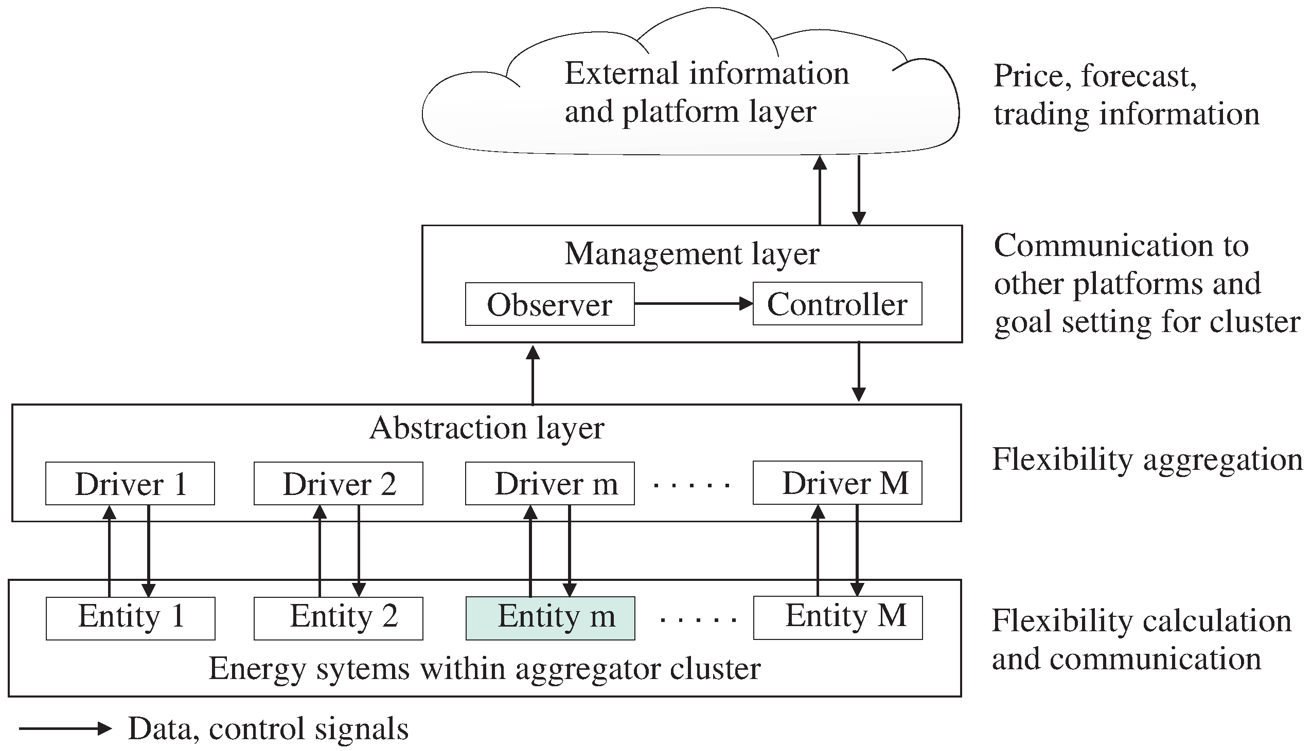
The aim of this article is the flexibility calculation of specific end-users without a pre-defined focus on possibly applied DSM mechanisms. This ensures the calculation of the full and reliable system flexibility of flexibility operators. With the developed approach, the communication of the maximum available short-term flexibility is possible for a couple of quarter hours into the future. Due to an end-user interface, the individual comfort requirements and flexibility sensitivity are taken into account. Thus, the end-user inputs reflect their individual willingness to participate in flexibility events. In order to reduce privacy and data security threats, an additional abstraction layer is implemented between the individual end-users and the flexibility operator. Figure 2 shows this additional abstraction layer to decouple the controlled entities from the management area following the architectural ideas from [7,8]. One additional purpose of the abstraction layer is the creation of a common understandable and generalized interface for the management layer. The function of the drivers is the conversion of locally used protocols in end-user systems to an understandable protocol, which can transmit the information to the management layer. With the proposed methodology and architecture of this article, a generalized flexibility value is introduced, which can easily be aggregated without the need for protocol conversions in the abstraction layer.

Figure 2.
General architecture of data and control signal exchange between entities in aggregator systems and management layer.
2.3. Market-Oriented Control of End-Users
The available flexibility on the consumer side can be utilized in several different ways, resulting in commercial benefits for the flexibility provider. The usage of the flexibility can be generally split into two main domains, grid-oriented and market-oriented services. The grid-oriented services are vital for a safe and solid operation of the grids which is the responsibility of transmission and distribution grid operators. Transmission system operators (TSOs) acquire capacity and energy reserves from both producers and consumers, in different forms for the frequency controls of their systems. The distribution system operators (DSOs), on the other hand, also utilize the grid services in order to maintain stability and to manage potential congestion of their grid. Opposed to these two examples, there is a variety of other use cases and business models for the usage of flexibility that do not define the benefits of the electrical grid as their primary goal, such as the usage of flexibility for energy trading at different electricity markets.
The potential for commercial usage of one’s flexibility depends on the available services, business models, and legislation in a specific country or region. A summary of available markets for the flexibility in Germany is given in Table 2. The frequency response reserves market is split into three main parts; primary containment reserve (primary control), frequency restoration reserve with automatic activation (secondary control), and frequency restoration reserve with manual activation (tertiary control or minute reserves). Due to numerous prerequisites for participation in one of the three parts of the market, the usage of consumer flexibility is technically feasible usually only within the tertiary control. Even then, participation occurs only via aggregator pools or within virtual power plants and not directly. A similar situation is encountered in the market for interruptible loads where the list of the numerous requirements makes participation possible only via aggregators or virtual power plants. Although technically feasible, the number of consumers participating in these two markets is still very low. The flexibility markets allow consumers and producers to offer their flexibility to the local DSO, usually via dedicated platforms. Different business cases, distinguishing in the criteria such as the market structure, reimbursement concept or pricing methods, have already been proposed and implemented [26]. Depending on the prerequisites for the specific flexibility market, small consumers such as households can participate via aggregators and virtual power plants or even directly as an independent flexibility provider. A further possibility for the commercial usage of flexibility is the trading at the electricity markets such as the EEX or the European Power Exchange (EPEX). Several studies show the potential for participation in the electricity markets for EV [27,28] and households [29,30], in the majority of cases via aggregation. The peer-2-peer markets represent another possibility of using the flexibility available on the local level, in the low voltage grid. Within these markets, the consumers can buy, whereas the prosumers can sell and buy energy locally, usually via a dedicated market platform, with or without involvement of external parties, such as aggregators or energy providing companies. In this paper, the usage of flexibility for both grid- or market-oriented purposes will be demonstrated.
Table 2.
Summary of available markets for the flexibility available in Germany, including their main characteristics.
3. PMS Extension Module for Flexibility Communication
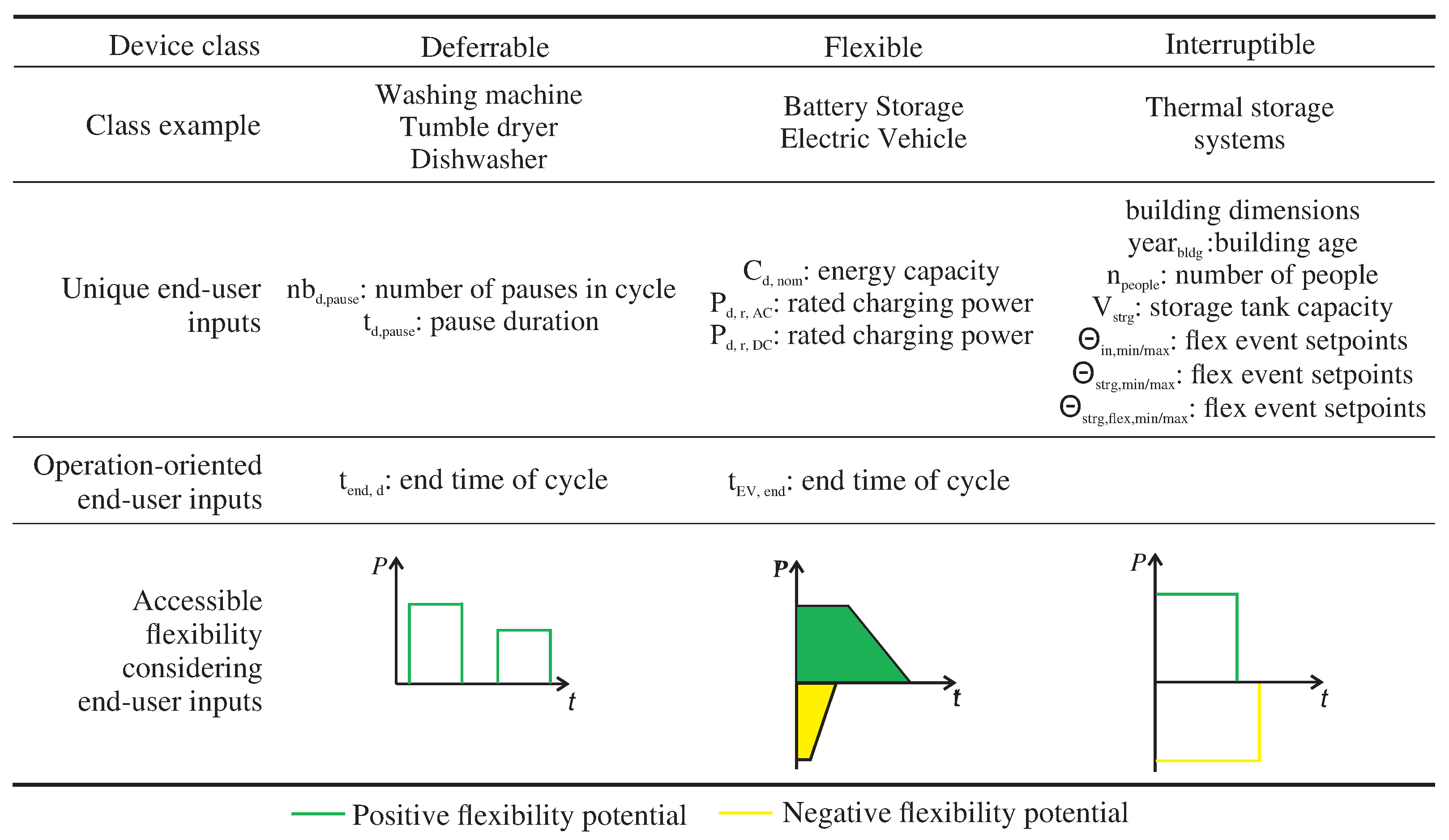
It is necessary to capture the in-time and short-term future states of contributing appliances and their state determining underlying parameters, in order to calculate a reliable, local flexibility potential to be communicated. By using this abstracted aggregated value, it is possible to communicate the flexibility potential of the associated appliances, i.e., participating residential and commercial end-users. By applying the aforementioned abstraction and aggregation layer in front of the management applications, a wide spectrum of DR programs can be realized. Figure 3 shows the generalized approach using end-user inputs for setting the flexibility calculation constraints. The flexibility approach applied to this work focuses on maximum available power over time provided by a general set of (1) deferrable, (2) interruptible, and (3) flexible loads shown in Figure 3, taking into account the power consumption patterns of the appliances, the current parameter states, and individual, specific end-user inputs for comfort purposes.
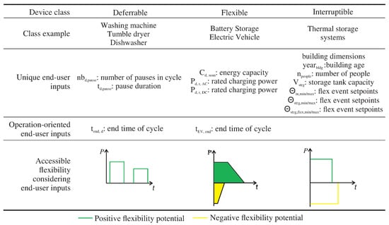
Figure 3.
Device classes and associated examples of devices with Power Management System inputs.
The overview in Figure 3 shows the applied device classes. However, the unique end-user inputs indicate a more complex contribution pattern of single appliances when considering additional degrees of freedom. Classic deferrable appliances can contribute as interruptible devices when considering short pauses in operation cycles [31]. With regard to short-term flexibility, flexible and interruptible loads contribute to possible power consumption deviations. The complement of additional loads, such as lighting or cooling devices, is possible.
3.1. Implementation into Secure Architecture
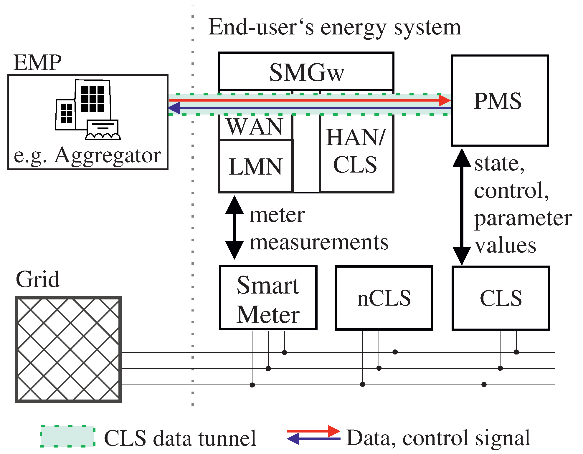
With the integration of an advanced metering infrastructure (AMI) Germany has implemented a highly secure communication device, called Smart Meter Gateway (SMGw), which enables communication and signal exchange between different entities surrounding the AMI [32]. A detailed overview of the infrastructure and related requirements, focusing on aspects of modeling and real-time simulation are presented in [33]. The communication and data exchange is established between the wide area network (WAN), including different external market participants (EMP), the home area network (HAN) with an end-user’s smart and controllable appliances and a visualization interface, and the local metrological network (LMN), consisting of metering devices for electricity. The LMN is also capable of including metering devices for other sectors, such as water or gas. For the communication to smart and controllable devices, so-called controllable local systems (CLSs), the SMGw offers an additional communication channel for a limited and certified set of EMPs. This additional transparent data channel allows the direct communication and data exchange to end-user controllable devices. For energy and power management purposes over a wide variety of different loads or RES, the connection to only one local central management system is beneficial. The information allocated by the local central management system to EMPs is independent from device specific protocols within the HAN devices. Besides this harmonized information allocation, only one device, the management system, has to be configured by the SMGw-administrator as CLS within the SMGw. Other smart and controllable devices are directly connected to the central management device. The proposed implementation is shown in Figure 4. Only CLS directly connects to the local central management system communicate state and parameter values. In contrast, non-CLS (nCLS) only contributes to the overall power consumption without the adjustment potential. By sending signals to the local central management system, the CLS operation is adjusted to met the pre-defined goals. The key parameter to be determined is the accessible amount of power that can be adjusted in the next hours. The need for a highly secure software and hardware architecture in the energy sector, discussed in [12,13], especially when concentrating on the demand side [16], has only been considered in a few cases [17]. With the developed methodology and the integration into the presented architecture, this gap can be closed.
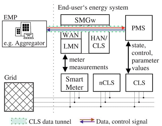
Figure 4.
Proposed implementation of flexibility communication and control into Smart Meter Gateway (SMGw) infrastructure, following the regulations from [32]. The external market participant (EMP) receives flexibility information through the transparent data tunnel functionality of the SMGw, connecting the wide area network (WAN) and the controllable local systems (CLSs). The power management system (PMS) adjust the CLS schedule, following EMP signals.
3.2. Methodology Description
We consider the time of the day represented by I intervals where and M participating end-users with . The power consumption of end-user m in interval i can be calculated according to Equation (2). Whereas is the non-adjustable power consumption, can be monitored and controlled for power adjustments through data and signal exchanges between smart devices and the PMS. Protocols like EEBUS or other protocols can be applied. However, the simple aggregated power consumption of smart devices is not addressable for the entire value, taking into account the specific appliance’s state and the state determining underlying parameters and their future development.
As an example, we consider a water heater with an attached storage tank. In order to meet the user’s comfort level, the water temperature is between two pre-defined thresholds, the lower and upper storage tank temperature. The modus operandi is such that the water heater will switch to the ON state in order to bring the water temperature to the upper threshold. An external switch OFF signal will lead to a cut in the heating process for only a short time interval as the temperature must be held above the lower temperature threshold for not harming end-user comfort constraints. The developed methodology takes into account not only the current state of the heater, but also the state determining parameters, such as the water and inner room temperature. An additional example of a dish washer can express the problem. The possibility to interrupt the operation cycle of the appliance for a pre-defined couple of minutes introduces , which sets the maximum duration the operation cycle of the dish washer can be interrupted for. Now, not only this value has to be considered. The additional value (see Figure 3) for the end time of operation needs to be integrated, when calculating the time length of flexibility’s availability. The general value and impact of pausing major household appliances is described in [34].
Taking into account the aforementioned examples, the controllable part of Equation (2) can be changed to Equation (3). The flexibility’s availability is expressed in a step time length of . Equation (3) shows the separation of the D CLS into two bins for accessibility greater (defined as ) and smaller (defined as ) . CLS being in bin contributes to flexibility events, as the others belonging to change their actual status before the possible event can take place.
Assuming that the separation into the two bins changes over time, can be written as the flexibility matrix with the abstracted information about accessible power, duration, and possible start time of flexibility events for end-user m, communicated at interval i. the flexibility matrix is shown in Equations (4) and (5). The row corresponds to the possible start time of the flexibility event, on the time basis of . Thus, the first possible allocation of the flexibility appears in min, taking into account the lack of immediate communication and reaction, and possible trading intervals on energy trading platforms. Column contains the possible duration of the flexibility event.
The exemplary value , sent at 7 p.m. for intervals (see Equation (6)), shows a accessible flexibility event starting at ( min) 7:45 p.m. Taking into account Equation (7) the duration can be calculated.
where
By sending the flexibility matrix repeatedly in a constant time interval of the accessible system flexibility can be updated for further consideration. The further reduction of rows is possible, when only information about the next possible flexibility event is needed. The information flow is shown in Figure 5. Beginning with the CLS, the PMS calculates the flexibility potential to fill the flexibility matrices. The here applied dimensions of are N = 4 and J = 6, which means a maximum forecast of 150 min with an event that starts in n = 4 (60 min) for then min. As the next step, the flexibility matrices, consisting of information about power, duration, and possible start time of the event, are sent to the abstraction and aggregation layer. By aggregating all connected entities m in the aggregator system the system flexibility can be transferred to the management layer operated in the aggregator backend. With information about accessible flexibility in the aggregator system, the exact flexibility offered in the markets, such as the intra-day spot market, can be realized. Reacting to power production uncertainty, the communicated flexibility can be used by DSO to ensure and restore a reliable system operation.
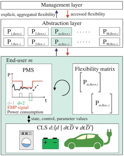
Figure 5.
Information flow in the presented methodology from the controllable local system to management layer.
To this point, Equations (2)–(5) only consider load reduction potential from turn-off appliances as generation substitute. Expanding the described method to appliances with an automated switching functionality, e.g., thermal or electric storage devices shown in Figure 3 an additional load capacity is added. Equation (8) shows this additional load potential. Considering the expected time of device d to stay in the current ON or OFF state, it can either belong to bin for a turn off flexibility and temporal ON state or to for turn on flexibility and temporal OFF state. Following the same suggestions as for Equation (3) only the flexibility, which is still accessible in and later is relevant for flexibility consideration. These devices belong to . The formulation of Equation (4) for a positive or negative flexibility potential of the end-user is introduced. As described above, shows the load reduction potential, whereas shows the load increase potential. The system flexibility potential is then for generation and for additional power demand. Whereas three device classes and their contributions to flexibility realization are shown in Figure 3, only interruptible and flexible devices are relevant for further consideration. This is because the flexibility matrices show the maximum possible deviation from the current power consumption.
3.3. Single Device Flexibility Calculation
Following the method explanations for flexibility aggregation developed in this work, this section describes the single device flexibility calculation for exemplary devices. Figure 3 shows the end-user’s unique and operation-oriented inputs for determining the flexibility for the applied devices. With the implementation of knowledge-based models of the applied appliances into PMS functionality, the interaction with the status-determining and monitored parameters can be locally evaluated to fill the flexibility matrices.
In the following section, the approach is presented with three exemplary appliances: electric heater systems, EVs, and so-called "white goods" devices. The following comprises a detailed reference device model for the end-user model and the PMS internal algorithm for flexibility calculation and communication. Other devices, such as lighting or cooling equipment, can be added to the PMS functionality under the same procedure as shown for the selected devices in the next section. The flexibility potential can be increased by adding more interruptible loads to the energy system.
3.3.1. Electric Heater System
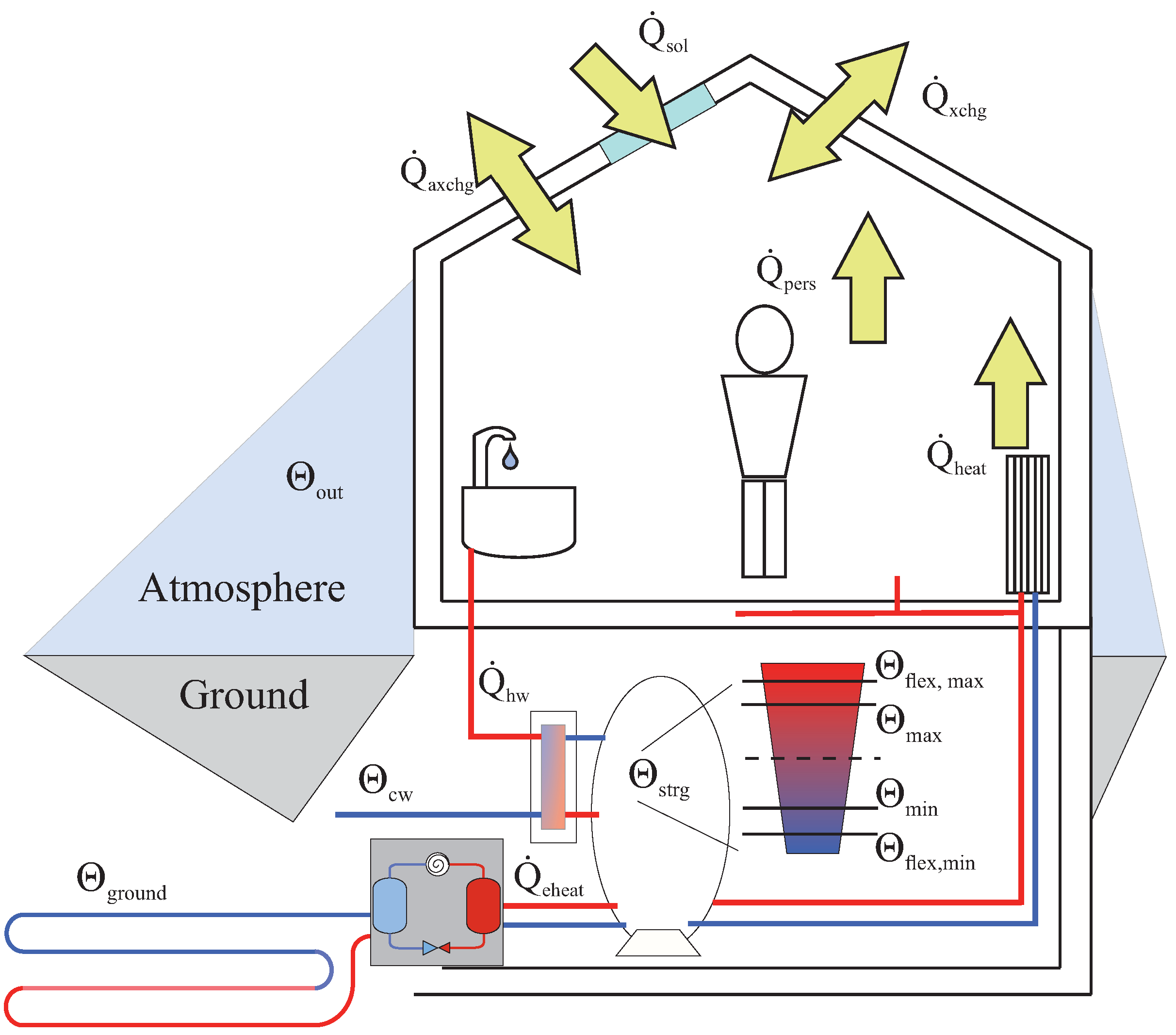
The thermal dynamic of buildings, following the same number of interval I, can be calculated through Equations (9) and (10) for the next step’s inner temperature and the water storage temperature , applied and validated in [33]. The additional parameters stated are the heat gain through windows , the heat gain arising from the heat flow from the hot water storage tank , which is positive for Equation (9) and negative for Equation (10), the heat gain from present persons and the heat capacities of storage tank , and rooms . The values and contain the thermal exchanges with the surrounding air caused by transmission through building components and direct ventilation. The hot water usage is covered by , whereas represents the electrical heater heat gain. The implementation of efficiencies is possible and can be applied to conversion and transportation losses. The needed temperatures and heat exchanges are shown in Figure 6 with a ground source heat pump system.
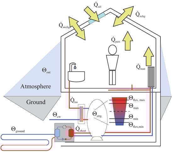
Figure 6.
Thermal dynamics within the applied heating model with outer , ground , and cold water temperature with normal and flexible setpoints for storage tank temperature .
Applying the flexibility methodology and end-user inputs from Figure 3 to the above-mentioned heating system, the remaining time until the storage tank temperature and the inner temperature reach the lower setpoints can be used as positive flexibility or generation equivalent, when ON. By calculating the energy difference between the current storage tank temperature and the lower temperature , the remaining time can be estimated. The parameter shows the width of the allowed storage temperature range and indicates the lower and upper allowed temperatures for heating operations. By adding a wider flexibility event dead band for the storage tank operation, an ancillary flexibility space can be added to the normal operation. This wider flexibility space is shown in Figure 6 for the storage tank temperature.
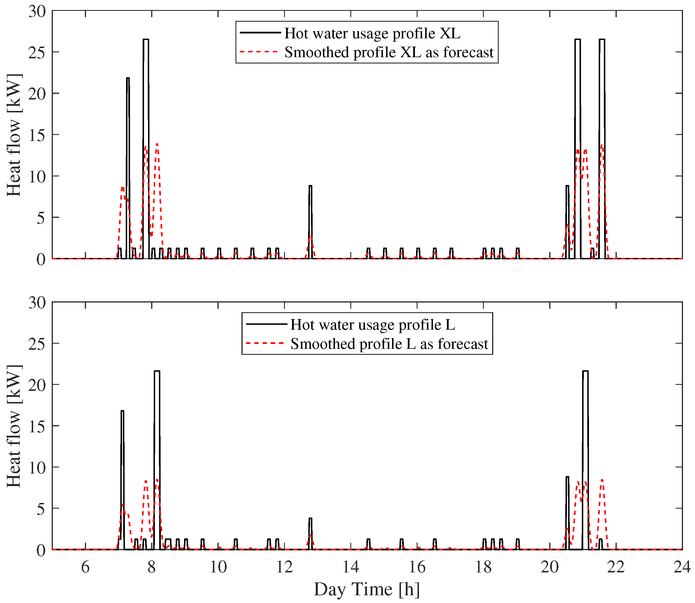
Relevant parameters for the estimation of flexibility are the assumed hot water usage for the next intervals and the heat transmission through the building components. The hot water usage profile is closely linked to the number of end-users in the building. By setting the number of people as PMS end-user input, one of three smoothed hot water usage profiles applied in [33] are implemented as hot water usage forecast . Through overlapping the three hot water usage profiles, a normalized hot water usage forecast profile is generated, which can depict a wide set of household configurations. By using Equation (11) the adjustment factor for each possible household configuration, taking into account the number of people, can be calculated. Different energy demands , for a defined number of people, can be used for the forecast adjustment. Figure 7 shows the original hot water usage profiles L and XL derived from [35] and the applied forecast profiles for PMS calculation with an end-user input for two/three people and four people, respectively.
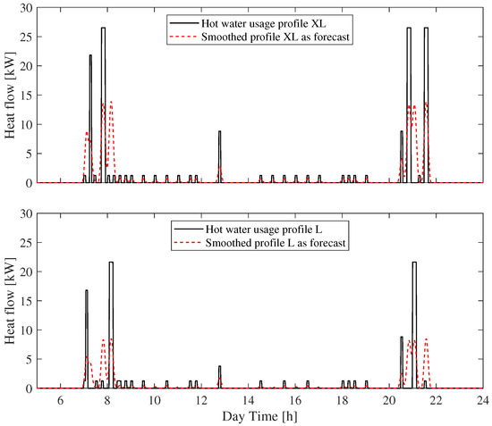
Figure 7.
Original hot water usage profile, XL and L, with an energy demand of 19.07 kWh and 11.655 kWh per day and smoothed profiles for PMS applications, based on data extracted from [35].
The additional end-user inputs containing building age and building dimensions influence the thermal transmission through the building or storage tank envelope . By setting PMS inputs for building age a generalized k-value is applied for thermal transmission, analyzed by [36] for the evolved building standards and corresponding k-values in Germany. These values for four different building standards are implemented in the real time simulation. On the one hand the implementation is performed for the electric heater and the thermal building model, by adjusting the averaged k-value for a component, stated in [36], with an allowed maximum 10% deviation normally distributed and on the other hand by the implementation of the averaged value into PMS functionality.
The remaining time until the lower energy level is reached for an interval i can be calculated using Equations (12) and (13). When in the OFF state, the remaining time until the upper energy level of the storage tank temperature is reached, can be calculated with Equations (14) and (15). For calculation, the actual temperature is defined as the starting energy level . The rated electrical power from the heater system itself and for the additional electric heating element , when installed for temperatures beneath the operation temperature , are used for calculating the electrical power during flexibility events with Equation (16). Following the same idea for inner room temperature, the remaining time until the inner room temperature reaches the lower or higher setpoint can be estimated.
With the two calculated time values, and , the flexibility matrix of Equation (4) can be filled. It is important to emphasize that the possible starting time of the flexibility event depends on the time values for normal operation and , because these values quantify the time until the status of the heating system will change to ON and OFF, respectively. The same issue is relevant for the duration of the flexibility event but in the opposite way. This is because the heating system can only add the inquired flexibility, when in the opposite status.
3.3.2. Electric Vehicle
The here applied EV model is based on the battery model as presented in [37] with Equations (17) for open circuit voltage (OCV), taking into account the actual state of charge (SOC) and Equation (18) for SOC calculation for next time step. The parameter values for the fitted OCV curve is shown in Table 3. Figure 8 shows the fitted OCV for the battery model applied to the simulated EV. The power for charging the EV is shown in Equation (20), using the charging behaviour switching point and the rated AC charging power of the EV. The marks the SOC value, where the constant current (CC) phase for charging an EV switches to the constant voltage (CV) phase with a power, which decreases monotonically until the SOC reaches the full capacity of the EV. The different charging characteristics for charging EVs are described in [38,39]. The specific parameter values for EV modeling are based on the VW e-Golf and the measurement results in [38]. Table 3 contains all applied values for battery and EV modeling within the simulation. The overall nominal battery capacity of the EV is calculated with Equation (19). The lost energy after arrival at home as the frequency of occurrence is implemented with the open access information from [40].
Table 3.
Parameters for the applied battery and EV model.
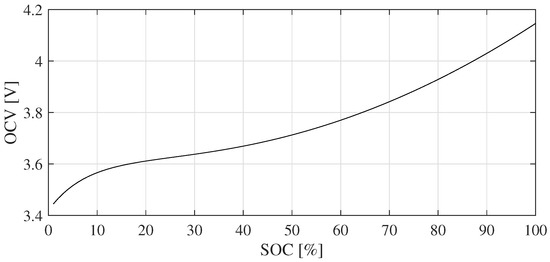
Figure 8.
OCV of one cell for the applied battery model to different SOC states for the modeled reference device EV.
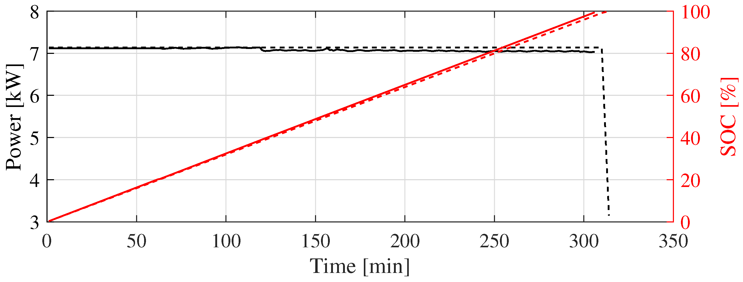
Applying the flexibility methodology and end-user inputs from Figure 3 to the EV charging process, the remaining time until the charging process has to start, is the maximum duration of the flexibility availability . Equation (21) shows the calculation of the possible flexibility event duration. As stated in [38,41] the linear SOC phase is recommended for controlling by EV charging coordinators, because the charging behaviour in the constant voltage phase is of a heterogeneous nature. Thus, the knowledge about the exact position of the is of high importance, when calculating the existing flexibility potential of EVs. In [38] a mathematical method for calculating the is presented for 11 kW charging stations. Datasets from different cars are analyzed to find dependencies between the and easy to capture vehicle-specific parameters. Equation (22) shows these dependencies between the and the charging power, both for AC and DC. With a linearized coherence the charging time can be estimated with knowledge about the charging power and battery capacity of the vehicle. The time share of the constant voltage phase of the overall charging time can be estimated with Equation (23). The parameter values for the fitted curves for the aforementioned Equations (22) and (23) can be found in Table 4. Figure 9 shows a measured charging profile and the forecast of the charging process, only using the unique end-user inputs for battery capacity and powers and . With the additional operation-oriented input for the end-user set end time of charging , equally distributed from 6 to 16 h, all relevant parameters for calculating the flexibility are captured.
with
Table 4.
Parameter values and RMSE for fitted curves, for calculating and the time share for decreasing power phase .
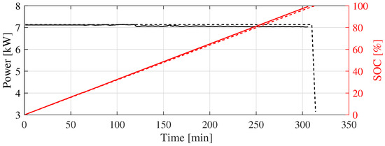
Figure 9.
VW e-Golf measured charging profile from SOC = 37% and extrapolated to SOC = 0% in straight lines with data from [38] and the pre-calculated charging profile based on the state of charge switching-point model in dashed lines.
When estimating possible power reductions to fill the flexibility matrices, the associated power consumption by the current SOC needs to be known. Then, a matrix , shown in Equation (24), can be calculated containing the pre-calculated minute-based charging process. For each minute from start to fully charged, the SOC and associated power consumption are defined as first and second dimensions, respectively. For the here applied VW e-Golf, the pre-calculated matrix has a length of 314 values for both SOC and charging power.
Applying the information from to a newly arrived EV, the remaining time until the EV is fully charged can be calculated with:
With the knowledge about the current SOC and the corresponding position q within the matrix all future minute-based power consumption can be extracted and used to communicate flexibility potential for the CC phase of the charging process. The measured CC phase for the VW e-Golf goes up to SOC = 100% and is estimated by Equation (22) at 99.1% with an absolute difference of 4 min.
3.3.3. White Goods
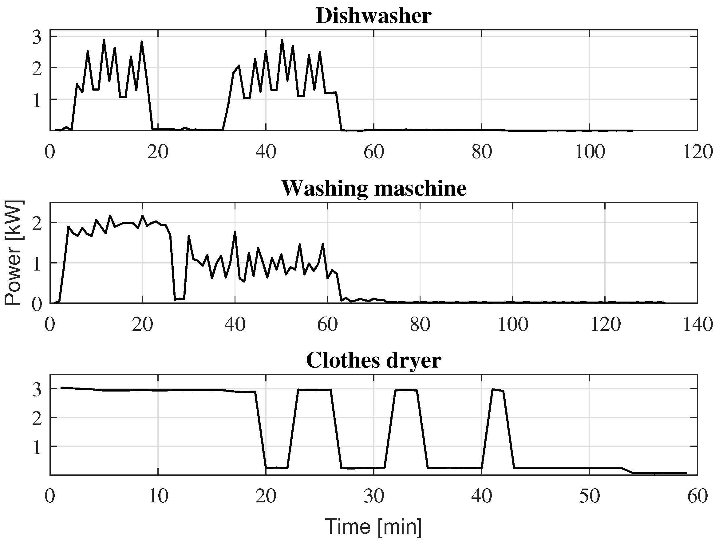
The integration of white goods into the simulation is based on the work of [33,42]. The power consumption during cycles are extracted from [34,43]. These integrated profiles are shown in Figure 10. For determining the flexibility potential from the white goods devices for filling the flexibility matrix, unique end-user, as well as operation-oriented inputs are necessary, as outlined in Figure 3. With the setting of the unique inputs for the maximum pause duration for white good device d and the maximum number of pauses during a cycle the flexibility potential can be calculated, under strict consideration of end-user’s comfort restrictions. With the additional operation-oriented input for the end-user set end time of cycle , which corresponds to the accepted delay time this additional constraint can be considered, when calculating the possible event duration. With a further restriction of a minimum run time of 15 min between the possible pauses, the flexibility matrix can be adjusted with the possible event start times and the duration, following Equation (26).
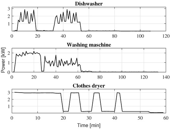
Figure 10.
Applied profiles of integrated white goods with data extracted from [34,43].
The power consumption of devices can be monitored with internal measurement equipment, as in EV supply equipment or with integrated smart plugs, as performed in [44]. With the protocol-based data exchange between devices and the central PMS, the power consumption can be monitored and forecasts can be calculated, when taking into account the starting time of the white goods device. With this information about power consumption, the flexibility matrix can be further adjusted. The operation-oriented end-user set end time of the cycle is extracted from [45] for all three implemented devices.
4. Use Case Scenario
The developed methodology was implemented into the set-up introduced in [33]. The aforementioned detailed Simulink device models for an EV, a heat pump system, a washing machine, a dishwasher, and a tumble dryer were used as reference devices. Thus, the associated specific operation and state conditions were monitored following the architecture of Figure 4. Table 5 shows the end-user’s unique inputs applied to the use case building composition. These end-user inputs were processed by the PMS functionality for calculating short-term flexibility. Additionally, the operation-oriented parameters set by the end-user and the underlying state determining parameters can be submitted by standardized protocols like EEBUS or OpenADR. The results are based on a simulation interval of three working days in spring.
Table 5.
Unique end-user inputs for PMS extension operation.
The calculated device specific flexibility values were modified following the proposed methodology described in Section 3 to fill the flexibility matrices from Equation (4). Utilizing the transparent data tunnel as central SMGw functionality, the flexibility matrices were allocated to interested EMPs within the WAN. The EMP is able to access the flexibility potential due to short-term forecast errors or trading at intra-day energy exchange markets. The specific usage of the offered flexibility is now not explicitly stated to demonstrate a wide spectrum of DSM measures.
4.1. Methodology Application on Electric Vehicle
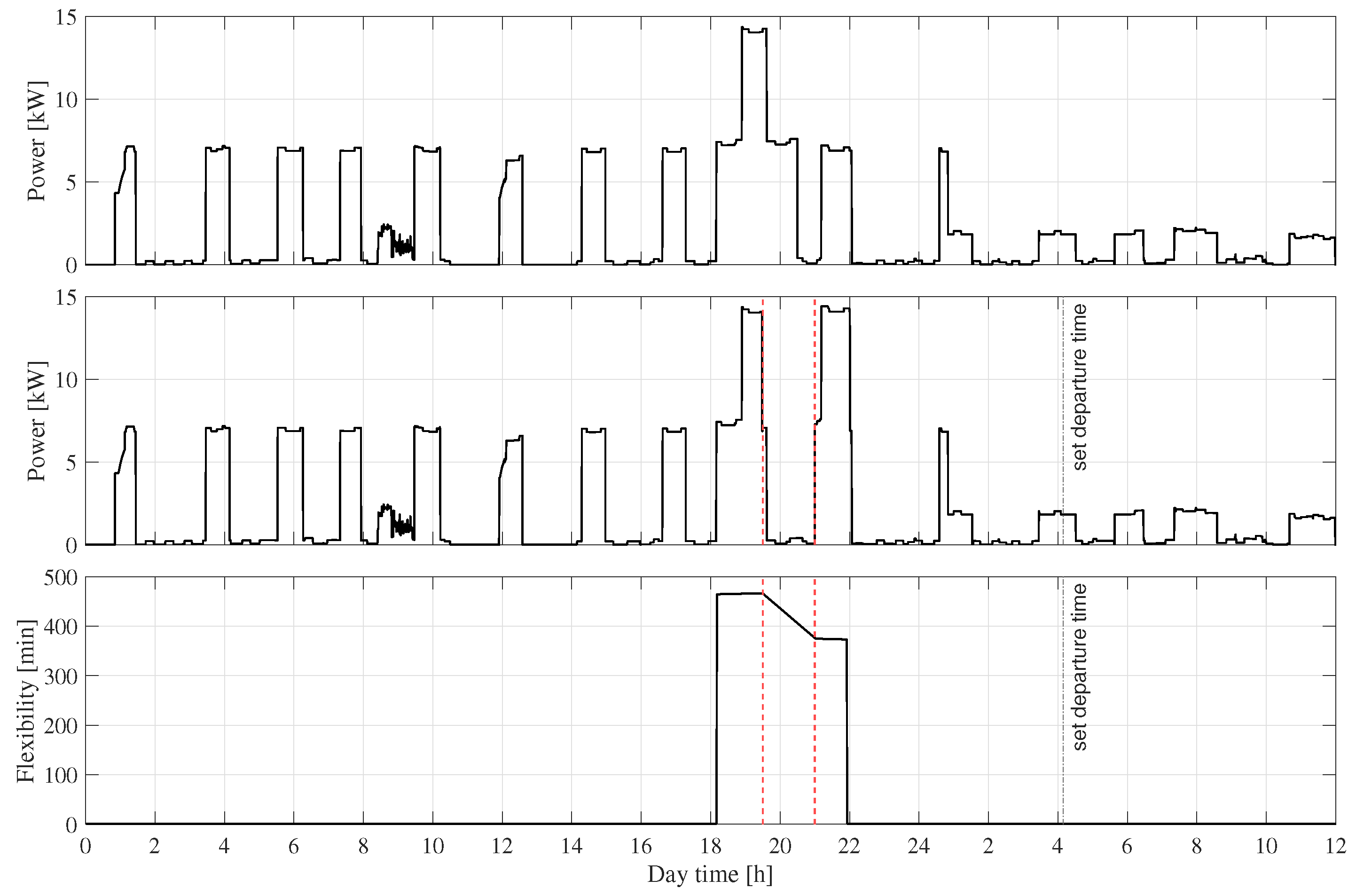
In Figure 11, a flexibility event was chosen by the EMP at the first day of the simulation interval, which includes the EV flexibility potential. The corresponding first row of the flexibility matrix for generation substitute is presented in Equation (27), depicting the positive flexibility matrix for a working day in spring. The flexibility matrix was sent at , which corresponds to 07:15 p.m. The communicated power reduction potential estimated with 7.128 kW was realised with a difference of 70 W. The load adjustment was realised in the communicated manner, without harming the end-user comfort settings, here defined as departure time.
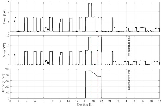
Figure 11.
Consumption profile for the use-case scenario without (top) and with flexibility event (middle) offering the EV flexibility with the calculated duration flexibility and end-user set departure time (bottom). The chosen flexibility event is marked by a red-dotted area.
4.2. Methodology Application on Heating System
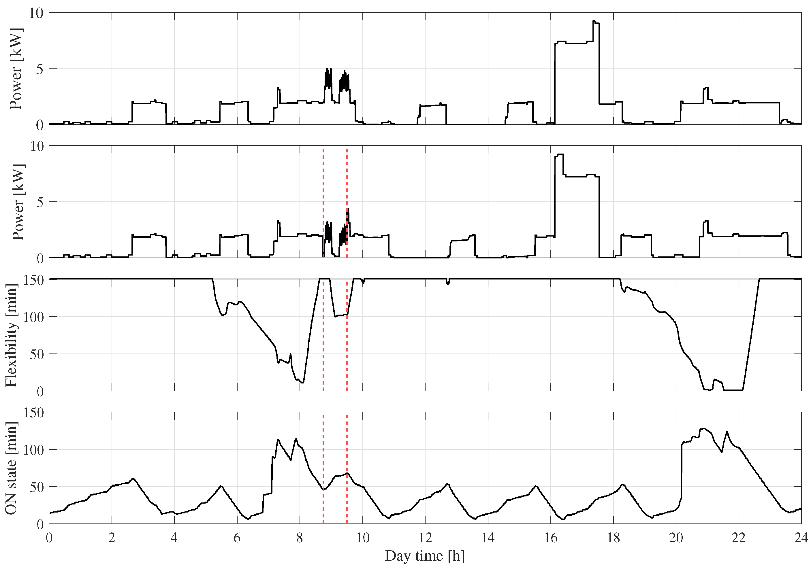
A second flexibility event was chosen by the EMP at the third day of the simulation interval with the help of a flexibility matrix sent at , which corresponds to 08:00 a.m. The third row of the flexibility matrix is depicted in Equation (28), showing a possible event with a duration of 45 min, starting at 08:45 a.m. In Figure 12 the realised flexibility event in comparison with the not realised flexibility event profile is shown. In addition, Figure 12 shows the calculated time until the lower flexible storage temperature is reached, which includes the possible event duration when turning to OFF state. Within the algorithm the maximum duration is set to 150 min, which means a possible extension of the flexibility matrix to entries. The highly relevant value for staying in ON state, shown in Figure 12 leads to possible flexibility events only when higher then 15 min, because only then the heat pump system could be turned to the OFF state. Due to the realised flexibility event the ensuing behaviour of the heat pump system changes compared to the profile without flexibility event. Assuming an increasing implementation of flexibility, usage profiles of devices or end-users influenced by flexibility events should not be used for flexibility evaluations, without knowing the exact flexibility event. Through the possible communication connection to different EMPs or contributions to different aggregator systems, the information about flexibility realisations and profile adjustments should be accessible to a wider spectrum of entities. Without this information, monitored profiles are hardly usable for getting more insight in flexibility potentials in energy systems.
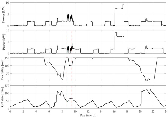
Figure 12.
Consumption profile for the use-case scenario without (top) and with flexibility event (second from top) offering the heat pump flexibility with the calculated duration event duration. The possible flexibility event duration (second from bottom) and the time until the upper operation temperature when in ON state is reached (bottom) with the flexibility event marked by a red-dotted area.
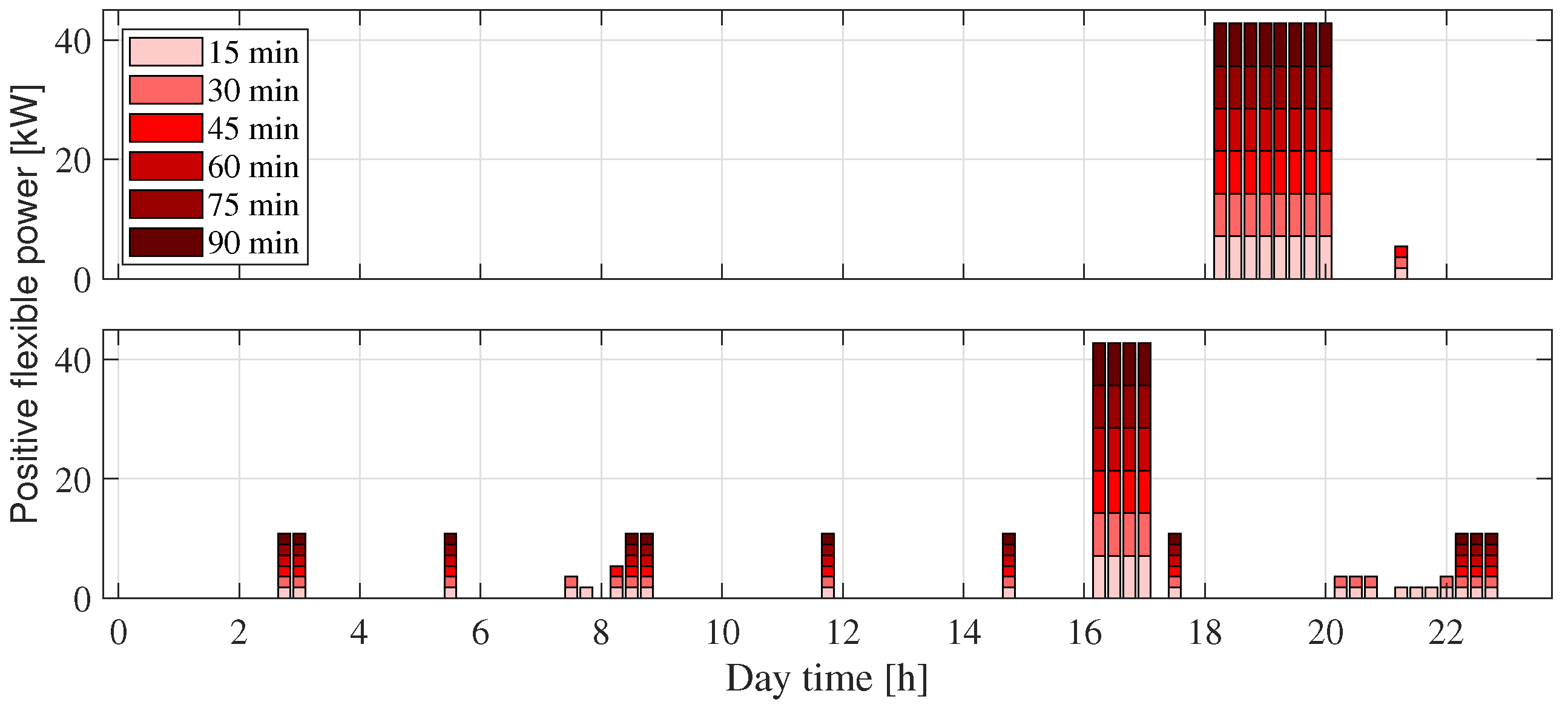
Figure 13 shows the calculated and communicated flexibility for the first day (top) and the third day (bottom) of the simulation without the aforementioned, realised flexibility events. It shows the first row of the flexibility matrix, which corresponds to a possible flexibility event starting in the next quarter. The height of the bars is not the overall potential. To extract the power potential, the height of the single duration needs to be extracted. For the first day, a noticeable result is the relatively small flexibility throughout the day. In particular, the heating system adds no flexibility to the overall potential. This occurs because of temperatures beneath the additional heater operation temperature, which leads to a relatively small turn ON duration. The flexibility only is accessible, when the heating system is ON for more then 15 min. Furthermore, the white goods devices add only very small contributions to the overall flexibility potential, because of the pause duration of only 15 min.
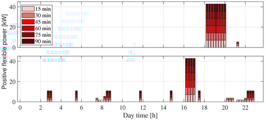
Figure 13.
Calculated and communicated flexibility for the first day (top) and third day (bottom) of the simulation, for the first row of the flexibility matrix, which corresponds to a flexibility event starting in the next quarter hour.
5. Discussion
With the presented flexibility studies categorization, the need for a flexibility calculation and aggregation method was exposed. This method should be able to communicate a reliable single device potential to flexibility operators as a new market role or existing market participants, such as DSOs or energy providers, without harming private data security of end-user energy systems. The participation capability of an end-user system with an exemplary set of appliances with a high penetration rate in household composition was shown. For this, a methodology was developed to calculate a reliable and accurate local flexibility potential and to communicate this in a generalized manner to external entities for market- or grid-oriented purposes. The applicability of the developed methodology was shown through a use case scenario on working days in the spring with a reduced set of end-user inputs that were easy to derive and implement into the PMS interface. Classified by unique and operation-oriented inputs, the local flexibility potential could be determined and communicated to external entities. With the consideration of local state-determining parameters of the selected devices, a reliable and accurate flexibility potential was calculated and sent. The flexibility system operator accessed the offered flexibility, due to market- or grid-specific information to place offers at flexibility markets or to restore grid stability, due to load or production forecast errors. The use cases show an accurate flexibility determination for the modeled electric vehicle up to 90 min and 45 min for the heat pump system, respectively, without harming end-user comfort settings. Interruptions were then possible for nearly the whole potential reduction time in the flexibility matrix, set on 90 min in the use case scenario. Compared to white good devices, electric heating systems and electric vehicles add noticeable shares of possible power reduction for longer time periods. In contrast to this, white goods devices are capable of very short term power reductions, taking into account the individual end-user settings for allowed pause duration, in the use case scenario of 15 min and end time of operation.
Embedding the developed method into the existing SMGw infrastructure ensures data security and privacy, tackling the most dangerous threats in the field of smart grid deployment in the energy sector. With consideration of end-user set inputs, the specific, local affinity to contribute to flexibility events can be taken advantage of, circumventing the need to apply a merely coarse-grained generalized end-user structure or model. The simulation results show the workflow of the approach and the applicability for accessing the communicated short-term flexibility. The approach is able to achieve detailed insights into short-term flexibility potential in the flexibility operator connected energy system.
To summarize the key findings, these are:
- Functionality of a PMS for calculating and communicating the local flexibility potential.
- Applicability of a short-term power consumption forecasting method for devices with a high penetration rate, with the help of easy to derive parameters.
- SMGw infrastructure is capable of flexibility matrix communication between end-user and external market participant.
- Accessing the communicated flexibility potential without harming end-user comfort constraints.
As part of future work, the upcoming implementation of the approach into larger energy systems with a wider set of end-users will prove the large-scale applicability and the impact on grid stability or short-term profit maximization for EMPs and participating end-users. Furthermore, a detailed sensitivity analysis on the calculated flexibility can be performed to quantify the impact of end-user input changes on the local flexibility potential.
Author Contributions
Conceptualization, F.H. and M.P.; methodology, F.H.; software, F.H. and A.J.; validation, F.H.; formal analysis, F.H. and A.J.; investigation, F.H., A.J. and M.P.; resources, D.S.; data curation, F.H.; writing—original draft preparation, F.H. and A.J.; writing—review and editing, M.P. and D.S.; visualization, F.H. and A.J.; supervision, D.S.; project administration, D.S.; funding acquisition, D.S. All authors have read and agreed to the published version of the manuscript.
Funding
The project called ’Electrify Buildings for Electric Vehicles’ is funded by the German Federal Ministry for Economic Affairs and Energy under the support code 01MZ18014F.
Institutional Review Board Statement
Not applicable.
Informed Consent Statement
Not applicable.
Data Availability Statement
Not applicable.
Conflicts of Interest
The authors declare no conflict of interest.
Abbreviations
The following abbreviations are used in this manuscript:
| AMI | advanced metering infrastructure |
| CC | constant current |
| CLS | controllable local system |
| CV | constant voltage |
| DR | demand response |
| DSM | demand side management |
| DSO | distribution system operator |
| EEX | European Energy Exchange |
| EMP | external market participant |
| EPEX | European Power Exchange |
| EV | electric vehicle |
| HAN | home area network |
| LMN | local metrological network |
| nCLS | non controllable local system |
| OCV | open circuit voltage |
| PMS | power management system |
| SMGw | smart meter gateway |
| SOC | state of charge |
| TSO | transmission system operator |
| WAN | wide area network |
References
- Mathieu, J.L.; Vaya, M.G.; Andersson, G. Uncertainty in the flexibility of aggregations of demand response resources. In Proceedings of the IECON 2013—39th Annual Conference of the IEEE Industrial Electronics Society, Vienna, Austria, 10–13 November 2013; pp. 8052–8057. [Google Scholar]
- Heider, F.; Plenz, M.; Schulz, D. Smart Meter Gateway based Demand Side Management (In German: Smart-Meter-Gateway-Basiertes Demand-Side-Management). In Hamburger Beiträge zum Technischen Klimaschutz; Helmut Schmidt University: Hamburg, Germany, 2020; pp. 49–55. [Google Scholar]
- Sadeghianpourhamami, N.; Demeester, T.; Benoit, D.F.; Strobbe, M.; Develder, C. Modeling and analysis of residential flexibility: Timing of white good usage. Appl. Energy 2016, 179, 790–805. [Google Scholar] [CrossRef] [Green Version]
- Mauser, I.; Mueller, J.; Foerderer, K.; Schmeck, H. Definition, Modeling, and Communication of Flexibility in Smart Buildings and Smart Grid. In Proceedings of the International ETG Congress 2017, Bonn, Germany, 28–29 November 2017; pp. 1–6. [Google Scholar]
- Petersen, M.K.; Edlund, K.; Hansen, L.H.; Bendtsen, J.; Stoustrup, J. A taxonomy for modeling flexibility and a computationally efficient algorithm for dispatch in Smart Grids. In Proceedings of the 2013 American Control Conference, Washington, DC, USA, 17–19 June 2016; pp. 1150–1156. [Google Scholar]
- Bagherzadeh, L.; Shahinzadeh, H.; Shayeghi, H.; Gharehpetian, G.B. A short-term energy management of microgrids considering renewable energy resources, micro-compressed air energy storage and DRPs. Int. J. Renew. Energy Res. 2019, 9, 1712–1723. [Google Scholar]
- Hirsch, C. Scheduling-Based Energy-Management in Smart Grids (in German: Fahrplanbasiertes Energiemanagement in Smart Grids). Ph.D. Thesis, KIT-Bibliothek, Karlsruhe, Germany, 2015. [Google Scholar]
- Allerding, F.; Schmeck, H. Organic smart home: Architecture for energy management in intelligent buildings. In Proceedings of the 2011 Workshop on Organic Computing (OC’11), Karlsruhe, Germany, 18 June 2011; Association for Computing Machinery: New York, NY, USA, 2011; pp. 67–76. [Google Scholar]
- Kokos, I.; Lamprinos, I. Demand response strategy for optimal formulation of flexibility services. In Proceedings of the Mediterranean Conference on Power Generation, Transmission, Distribution and Energy Conversion (MedPower 2016), Belgrade, Serbia, 6–9 November 2016. [Google Scholar]
- Fleischle, F.; Kaniut, M.; Geißler, M.; Winnik, S. Digitization in the Energy Transition. Modernization and Progress Barometer on the Degree of Digitization of the Grid-Bound Energy Industry (In German: Barometer Digitalisierung der Energiewende. Modernisierungs- und Fortschrittsbarometer zum Grad der Digitalisierung der leitungsgebundenen Energiewirtschaft) Prepared on Behalf of the Federal Ministry for Economic Affairs and Energy, Ernst & Young. 2020. Available online: https://www.bmwi.de/Redaktion/DE/Publikationen/Studien/barometer-digitalisierung-der-energiewende-berichtsjahr-2019.pdf (accessed on 20 November 2021).
- Ayadi, F.; Colak, I.; Garip, I.; Bulbul, H.I. Impacts of Renewable Energy Resources in Smart Grid. In Proceedings of the 2020 8th International Conference on Smart Grid (icSmartGrid), Paris, France, 17–19 June 2020; pp. 183–188. [Google Scholar]
- Hossein Motlagh, N.; Mohammadrezaei, M.; Hunt, J.; Zakeri, B. Internet of Things (IoT) and the Energy Sector. Energies 2020, 13, 494. [Google Scholar] [CrossRef] [Green Version]
- Li, Z.; Shahidehpour, M.; Aminifar, F. Cybersecurity in Distributed Power Systems. Proc. IEEE 2017, 105, 1367–1388. [Google Scholar] [CrossRef]
- Durillon, B.; Davigny, A.; Kazmierczak, S.; Barry, H.; Saudemont, C.; Robyns, B. Demand Response Methodology Applied on Three-Axis Constructed Consumers Profiles. In Proceedings of the 2019 International Conference on Smart Energy Systems and Technologies (SEST), Porto, Portugal, 9–11 September 2019; pp. 1–6. [Google Scholar]
- Wohlfarth, K.; Klingler, A.-K.; Eichhammer, W. The flexibility deployment of the service sector—A demand response modelling approach coupled with evidence from a market research survey. Energy Strategy Rev. 2020, 28, 100460. [Google Scholar] [CrossRef]
- Chen, L.; Ma, L.; Liu, N.; Wang, L.; Liu, Z. Parameter tampering cyberattack and event-trigger detection in game-based interactive demand response. Int. J. Electr. Power Energy Syst. 2022, 135, 107550. [Google Scholar] [CrossRef]
- Hamwi, M.; Lizarralde, I.; Legardeur, J. Demand response business model canvas: A tool for flexibility creation in the electricity markets. J. Clean. Prod. 2021, 282, 124539. [Google Scholar] [CrossRef]
- Kara, E.C.; Tabone, M.D.; MacDonald, J.S.; Callaway, D.S.; Kiliccote, S. Quantifying flexibility of residential thermostatically controlled loads for demand response. In Mani Srivastava (Hg.): Proceedings of the 1st ACM Conference on Embedded Systems for Energy-Efficient Buildings. SenSys ’14: The 12th ACM Conference on Embedded Network Sensor Systems. Memphis Tennessee; ACM: New York, NY, USA, 2014; pp. 140–147. [Google Scholar]
- González, N.; Calatayud, P.; Arcos, L.; Trujillo, A.; Pellicer, M.G.; Quijano-López, A. Optimal Participation of Aggregated Residential Customers in Flexibility Markets. In Proceedings of the 8th International Conference on Smart Grid (icSmartGrid), Paris, France, 17–19 June 2020; pp. 43–47. [Google Scholar]
- Afzalan, M.; Jazizadeh, F. Residential loads flexibility potential for demand response using energy consumption patterns and user segments. Appl. Energy 2019, 254, 113693. [Google Scholar] [CrossRef]
- Herre, L.; Kazemi, S.; Söder, L. Quantifying flexibility of load aggregations: Impact of communication constraints on reserve capacity. IET Gener. Transm. Distrib. 2020, 14, 5211–5218. [Google Scholar] [CrossRef]
- Kafazi, I.E.; Bannari, R.; Hernández, A.C.L. Optimization Strategy Considering Energy Storage Systems to Minimize Energy Production Cost of Power Systems. Int. J. Renew. Energy Res. (IJRER) 2018, 8. [Google Scholar] [CrossRef]
- Wang, Z.; Munawar, U.; Paranjape, R. Stochastic Optimization for Residential Demand Response under Time of Use. In Proceedings of the 2020 IEEE International Conference on Power Electronics, Smart Grid and Renewable Energy (PESGRE2020), Cochin, India, 2–4 January 2020. [Google Scholar]
- Shen, F.; Wu, Q.; Jin, X.; Zhou, B.; Li, C.; Xu, Y. ADMM-based market clearing and optimal flexibility bidding of distribution-level flexibility market for day-ahead congestion management of distribution networks. Int. J. Electr. Power Energy Syst. 2020, 123, 106266. [Google Scholar] [CrossRef]
- Ayón, X.; Gruber, J.K.; Hayes, B.P.; Usaola, J.; Prodanović, M. An optimal day-ahead load scheduling approach based on the flexibility of aggregate demands. Appl. Energy 2017, 198, 1–11. [Google Scholar] [CrossRef] [Green Version]
- Valarezo, O.; Gomez, T.; Chaves-Avila, J.P.; Lind, L.; Correa, M.; Ziegler, D.U.; Escobar, R. Analysis of New Flexibility Market Models in Europe. Energies 2021, 14, 3521. [Google Scholar] [CrossRef]
- Naharudinsyah, I.; Limmer, S. Optimal Charging of Electric Vehicles with Trading on the Intraday Electricity Market. Energies 2018, 11, 1416. [Google Scholar] [CrossRef] [Green Version]
- Kern, T.; Dossow, P.; von Roon, S. Integrating Bidirectionally Chargeable Electric Vehicles into the Electricity Markets. Energies 2020, 13, 5812. [Google Scholar] [CrossRef]
- Ahmad, A.; Khan, A.; Javaid, N.; Hussain, H.M.; Abdul, W.; Almogren, A.; Alamri, A.; Niaz, I.A. An Optimized Home Energy Management System with Integrated Renewable Energy and Storage Resources. Energies 2017, 10, 549. [Google Scholar] [CrossRef] [Green Version]
- Schwabender, D.; Corinaldesi, C.; Lettner, G.; Auer, H. Business cases of aggregated flexibilities in multiple electricity markets in a European market design. Energy Convers. Manag. 2021, 230, 113783. [Google Scholar] [CrossRef]
- Nistor, S.; Wu, J.; Sooriyabandara, M.; Ekanayake, J. Capability of smart appliances to provide reserve services. Appl. Energy 2015, 138, 590–597. [Google Scholar] [CrossRef] [Green Version]
- Federal Office for Information Security. Technical Guideline BSI TR-0309-1. Requirements for the Interoperability of the Communication Unit of a Intelligent Metering System (In German: Technische Richtlinie BSI TR-03109-1, Anforderungen an Die Interoperabilität der Kommunikationseinheit Eines Intelligenten Messsystems). 17 September 2021. Version 1.1. Available online: https://www.bsi.bund.de/SharedDocs/Downloads/DE/BSI/Publikationen/TechnischeRichtlinien/TR03109/TR03109-1.pdf (accessed on 10 November 2021).
- Heider, F.; Plenz, M.; Becker, D.; Schulz, D. Residential Load Modeling for Energy Application and Integration Studies in the Framework of Smart Meter Gateways. In Proceedings of the Conference on Sustainable Energy Supply and Energy Storage Systems (NEIS 2020), Hamburg, Germany, 14–15 September 2020; pp. 1–8. [Google Scholar]
- Pipattanasomporn, M.; Kuzlu, M.; Rahman, S.; Teklu, Y. Load Profiles of Selected Major Household Appliances and Their Demand Response Opportunities. IEEE Trans. Smart Grid 2014, 5, 742–750. [Google Scholar] [CrossRef]
- German Institute for Standardization. Heat Pumps with Electrically Driven Compressors—Testing, Performance Rating and Requirements for Marking of Domestic Hot Water Units; German Version EN 16147:2017 + AC:2017, DIN EN 16147:2017-08; German Institute for Standardization: Berlin, Germany, 2017. [Google Scholar]
- Kallert, A.; Egelkamp, R.; Schmidt, D. High Resolution Heating load Profiles for Simulation Analysis of Small Scale Energy Systems. In Proceedings of the 16th International Symposium on District Heating and Cooling, Hamburg, Germany, 9–12 September 2018. [Google Scholar]
- Baccouche, I.; Jemmali, S.; Manai, B.; Omar, N.; Amara, N.E.B. Improved OCV Model of a Li-Ion NMC Battery for Online SOC Estimation Using the Extended Kalman Filter. Energies 2017, 10, 764. [Google Scholar] [CrossRef] [Green Version]
- Heider, F.; Jahic, A.; Plenz, M.; Schulz, D. A generic EV charging model extracted from real charging behaviour (in Review). In Proceedings of the 2022 IEEE IAS Global Conference on Emerging Technologies (GlobConET), Online, 20–21 May 2022. [Google Scholar]
- Newe, H.; Deters, S.; Saiju, R. Analysis of Electrical Charging Characteristics of Different Electric Vehicles Based on the Measurement of Vehicle-specific Load Profiles, NEIS 2019. In Proceedings of the Conference on Sustainable Energy Supply and Energy Storage Systems, Hamburg, Germany, 19–20 September 2019; pp. 1–6. [Google Scholar]
- ElaadNL Open Datasets: ElaadNL Open Datasets for Electric Mobility Research. Update April 2020. Available online: https://platform.elaad.io/analyses/ElaadNL_opendata.php (accessed on 5 November 2021).
- Marra, F.; Yang, G.Y.; Larsen, E.; Rasmussen, C.N.; You, S. Demand profile study of battery electric vehicle under different charging options. In Proceedings of the 2012 IEEE Power and Energy Society General Meeting, San Diego, CA, USA, 22–26 July 2012; pp. 1–7. [Google Scholar]
- Avdevicius, E.; Heider, F.; Eskander, M.; Schulz, D. Smart Grid Residential Load Modeling for Real-time Applications. In Proceedings of the NEIS 2021 Conference on Sustainable Energy Supply and Energy Storage Systems, Hamburg, Germany, 13–14 September 2021; pp. 1–8. [Google Scholar]
- Open Power System Data. Data Package Household Data. Version 2020-04-15. 2020. Available online: https://data.open-power-system-data.org/household_data/2020-04-15/ (accessed on 6 November 2021).
- Zhai, S.; Wang, Z.; Yan, X.; He, G. Appliance Flexibility Analysis Considering User Behavior in Home Energy Management System Using Smart Plugs. IEEE Trans. Ind. Electron. 2019, 66, 1391–1401. [Google Scholar] [CrossRef]
- Fanitabasi, F.; Pournaras, E. Appliance-Level Flexible Scheduling for Socio-Technical Smart Grid Optimization. IEEE Access 2020, 8, 119880–119898. [Google Scholar] [CrossRef]


Publisher’s Note: MDPI stays neutral with regard to jurisdictional claims in published maps and institutional affiliations. |
© 2022 by the authors. Licensee MDPI, Basel, Switzerland. This article is an open access article distributed under the terms and conditions of the Creative Commons Attribution (CC BY) license (https://creativecommons.org/licenses/by/4.0/).