Experimental Study on Temporal and Spatial Evolutions of Temperature Field of Double-Pipe Freezing in Saline Stratum with a High Velocity

Abstract

Freezing construction in saline stratum under the action of groundwater is typical. To study the coupling effect of the groundwater velocity and salinity on the freezing in saline stratum, the freezing temperature of saline sand with different salinities was obtained through experiments. A controllable velocity double-pipe freezing physical model test system for saline sand was established. The temperature distribution in saturated saline sand under different salinities and velocities were studied. The test results showed that the temporal and spatial evolutions of the temperature field were affected by the velocity and salinity. Under the same boundary temperature, the higher the salinity, the lower the temperature at the measuring point on the main surface and interface. The overlapping time varies significantly. The analysis results showed that the larger velocity and the higher the salinity, the longer the overlapping time. The velocity and salinity inhibited the development of the frozen curtain. Under different test conditions, the development rate of the freezing curtain area was in the range of 3987–15,246 mm²/h.

1. Introduction

A soil is called saline stratum when the total soluble salt in the soil mass is greater than 0.3%, and it has engineering characteristics such as solution subsidence, salt swelling, and corrosion [1]. Saline soil is distributed worldwide. In China, it is mainly distributed in coastal and northwest areas [2,3,4,5]. Saline stratum exhibits water–salt migration and frost heaving, which have a negative impact on the artificial stratum freezing method. During the freezing process, the salt in the stratum migrates with the water, which changes the concentration and distribution of the water and salt, and consequently affects the thermodynamic characteristics of the stratum [6,7,8]. The distribution of the temperature field and the development of the frozen curtain have different characteristics. Research on the development law of freezing in saline stratum can help expand the application scope of the freezing method and improve the freezing efficiency of the saline stratum.

Many scholars have studied the freezing in saline stratum. Bing et al. [9] introduced laboratory test results of the freezing point of saline soil. The results showed that the freezing point decreases with the increase in the salinity and water content. Wan et al. [10], Wu et al. [11], and Xiao et al. [12] established a calculation formula for the freezing temperature corresponding to different soil properties. Zhai et al. [13,14] proposed a new model as the explanation for water flow in unsaturated soil. Geng et al. [15] used the finite element method to simulate the migration of salt in water -bearing strata. Xu et al. [16] studied the coupled water-heat solute transport process by numerical simulation and discussed the dynamic changes in the unfrozen water content and the effects of freezing point on thermal, water, and salinity profiles. Zhang et al. [17] proposed a water -heat coupling model suitable for saline soil, and the accuracy of this model was supported by measured data. Wan et al. [18] developed a new model to explore the dynamic variation characteristics of the thermal conductivity of saline soils. Ye et al. [19] simulated the effect of groundwater salinity on the freezing effect and reached the conclusion that when the groundwater salinity is greater than 4%, the effect of salt cannot be ignored. At the same time, most of the above studies only considered the velocity or salinity. It will be meaningful to consider the above two factors at the same time.

Clearly, research on the freezing of saline soil mainly focused on analyzing its basic thermodynamic characteristics, and a numerical simulation is typically used to analyze the temperature field. Compared with numerical simulations, experimental methods were also often used to study engineering problems. In this study, a typical saturated coastal saline stratum was considered, including saline soil freezing conditions under different velocities and salinities. A set of large-scale physical model similarity tests was designed. Based on a test platform, freezing tests were conducted in saturated saline sand under different groundwater seepage velocities (hereinafter referred to as velocity) and salt solution concentration (hereinafter referred to as salinity). Combined with the research on the thermophysical characteristics of the sand layer, the development and distribution characteristics of the temperature field and the development law of the frozen curtain were determined. The test results provide references for freezing construction and design in saline stratum.

2. Freezing Point Test of Similar Materials in Saline Layer

2.1. Test Method and Scheme

To successfully conduct research on the freezing characteristics of saline stratum, it is necessary to study the thermophysical characteristics of saline stratum materials, among which the freezing temperature is an important parameter for the research and is a basis for analyzing the spatiotemporal development characteristics of the freezing curtain. The freezing temperature can be determined using four ways: based on the changes in the potential, resistance, heat, and temperature. Among them, the judgment method marked by the temperature is widely used owing to its simple and intuitive advantages. Figure 1 shows the temperature–time curve when soil is cooled and frozen [9]. The soil experiences four stages in the cooling process, among which the constant stage is the free water freezing stage, and the corresponding temperature is considered the freezing temperature [20,21,22].

Quartz sand (hereinafter referred to as sand) material commonly used as the filling layer in freezing model tests was selected for the research. The saturated volume water content of the selected sand layer is 20% [23], and the other properties of the sand layer are reported in

Table 1. Physical properties of the sand.

Particle Size (mm)	Dry Density (kg/m3)	Porosity	Saturated Moisture Content	Permeability Coefficient (m/s)
0.5 ± 0.15	1612	0.32	20%	2.28 × 10−4

. NaCl was selected as the salt source. Considering that the average salinity of seawater is 3.5%, the saline solution with mass salinities (hereinafter referred to as salinities) of 0%, 1%, 2%, 3%, 4%, 5%, 6%, and 7% was prepared for the test. Based on the saturated volume water content, the relationship between the salinity of the solution and the salinity of the saturated salt sand can be obtained, as listed in

Table 2. Relationship between salinities of solution and salinities of saline sand.

Salinities of the Solution	0%	1%	2%	3%	4%	5%	6%	7%
salinities of saline sand	0%	0.216%	0.435%	0.660%	0.889%	1.122%	1.362%	1.605%

. The configured salt sand covers low saline soil (salinity of saline sand 0.3–1.5%) and medium saline soil (salinity of saline sand 1.5–5.0%) [24]. The test was conducted with NaCl crystal powder (purity > 99%), and the solution was prepared with water from the municipal pipe. Due to the low ion content in the water, the influence of existing ions was no longer considered in the configuration and calculation [25]. The so-called 0% solution was directly prepared with municipal water source without adding NaCl crystal powder. In the following analysis, the salinity refers to the salinity of the salt solution, which can be converted to the salinity of saline soil.

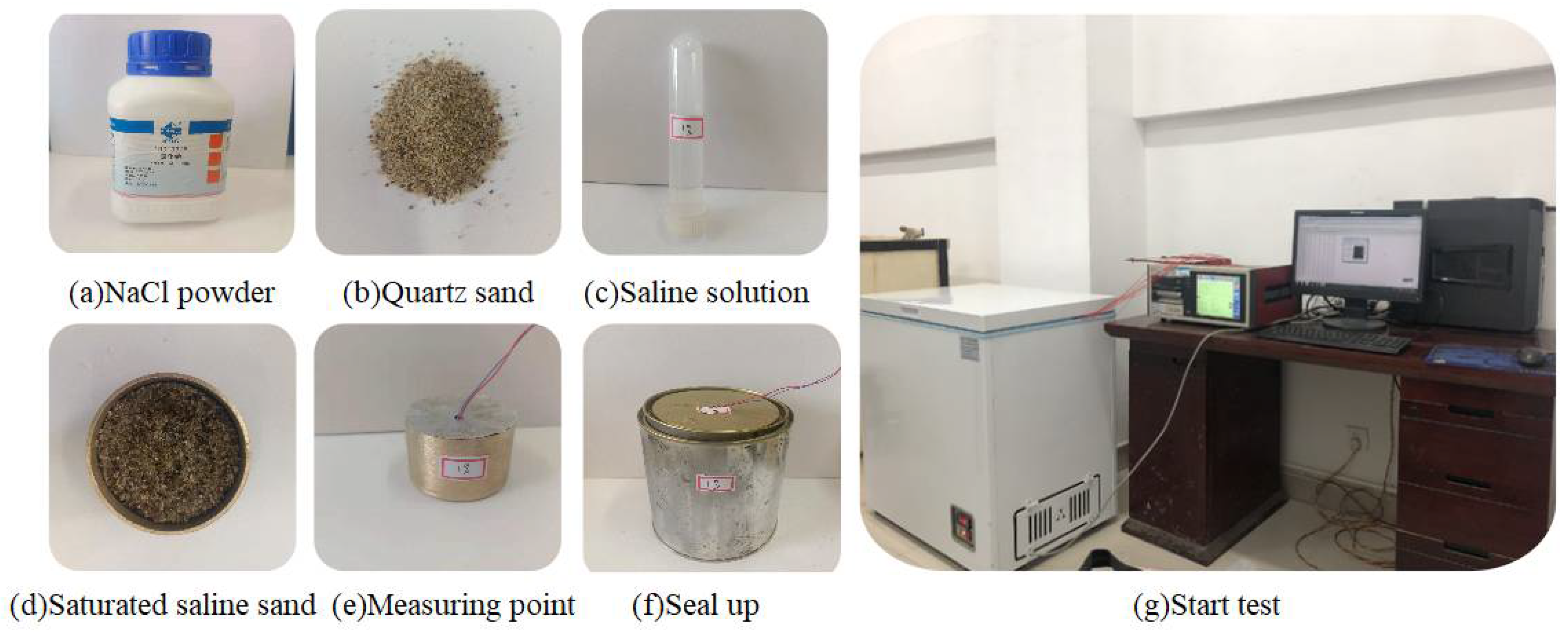
2.2. Experimental Equipment and Steps

The test included two systems: a low-temperature control system and a data acquisition and storage system. The low-temperature control system mainly included a DW-50 low temperature test chamber. The DW-50 has an accurate temperature control capability that can maintain a temperature from 0~−50 °C. The temperature control accuracy was 0.1 °C. The data acquisition system was composed of a TDS602 data acquisition instrument and T-type copper-constantan thermocouples. The temperature measurement accuracy was 0.1 °C and it can measure the temperature in the range of −100~400 °C. TDS602 was manufactured by Tokyo Sokki Kenkyuio Co., Ltd. It has the function of real-time scanning and multi-point measurement. The data storage and analysis system could record the data every 10 s. During the test, the solution was first prepared and then mixed with dry sand. A uniformly mixed saturated water-bearing sand was placed at the center of the metal container, and wrapped with dry sand after sealing. The measuring point passed through the metal cover to the center of the sand. Figure 2 shows the sample configuration and test system.

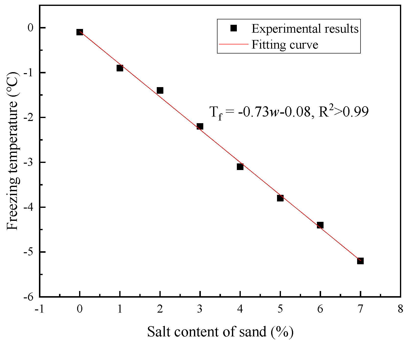
2.3. Analysis of Test Results

The rapid cooling scheme was adopted. the sample temperature before freezing was 11 °C. The temperature of the low-temperature test chamber was set to −22.0 °C during the test. and the sample was placed at the center of the low-temperature test chamber after the temperature stabilized. The cooling test was conducted on eight groups of samples twice to obtain the temperature–time curve of saline sand under different salinities. As Figure 3 shown, there are four stages in the cooling process of the sand samples, and the higher the salinity, the longer the supercooling stage, the longer the duration of the constant section, and the lower the corresponding freezing temperature, that is, for saturated sand samples, the higher the salinity, the lower the freezing temperature of the sand samples. The freezing temperature of sand under different salinities can be obtained from the above temperature reduction curve. The freezing temperature of the sand sample is plotted as shown in Figure 4.

Figure 4 shows that when the salinity is 0%, the freezing temperature of the sand is −0.1 °C, which is consistent with the existing research results [23] and shows the correctness of the test method and the reliability of the data. The salinity has an evident effect on the freezing temperature of sand. Through the fitting of the test data, a strong linear relationship can be seen between the freezing temperature T_f and salinity s. It can be considered that within the test range, the following equation is satisfied:

$$T_{\mathrm{f}}=-0.73s- 0.08$$

(1)

3. Model Test of Saline Sand under Different Velocities

3.1. Model Test Scheme

For the freezing of the saline sand, different velocities and salinities were considered. Considering the low salinity in the project, three salinities of 0%, 2%, and 4% were selected. At the same time, considering the environmental conditions of the saline soil, the test velocities were determined as 0, 3 and 6 m/d. Based on the above analysis, a large test platform was built, as shown in Figure 5. In Figure 5, from left to right, they were the temperature acquisition and analysis system, the core test area, the constant-temperature brine circulation system and freezing circulation system. The core test area was densely filled with the above sand. A constant-temperature brine circulation system with a flowmeter and a temperature controller were employed to achieve directional stable constant-speed horizontal water flow. The salinity can be controlled by using a salinity meter.

Table 3. Dimensions of the model test.

Geometric Similarity Ratio	Temperature Similarity Ratio	Time Similarity Ratio	Model Test Size	Freezing Pipe Radius	Freezing Pipe Spacing
1/3	1	1/3	1.5 m × 2 m × 1 m	0.02 m	0.4 m

presents some of the parameters of the test platform [26].

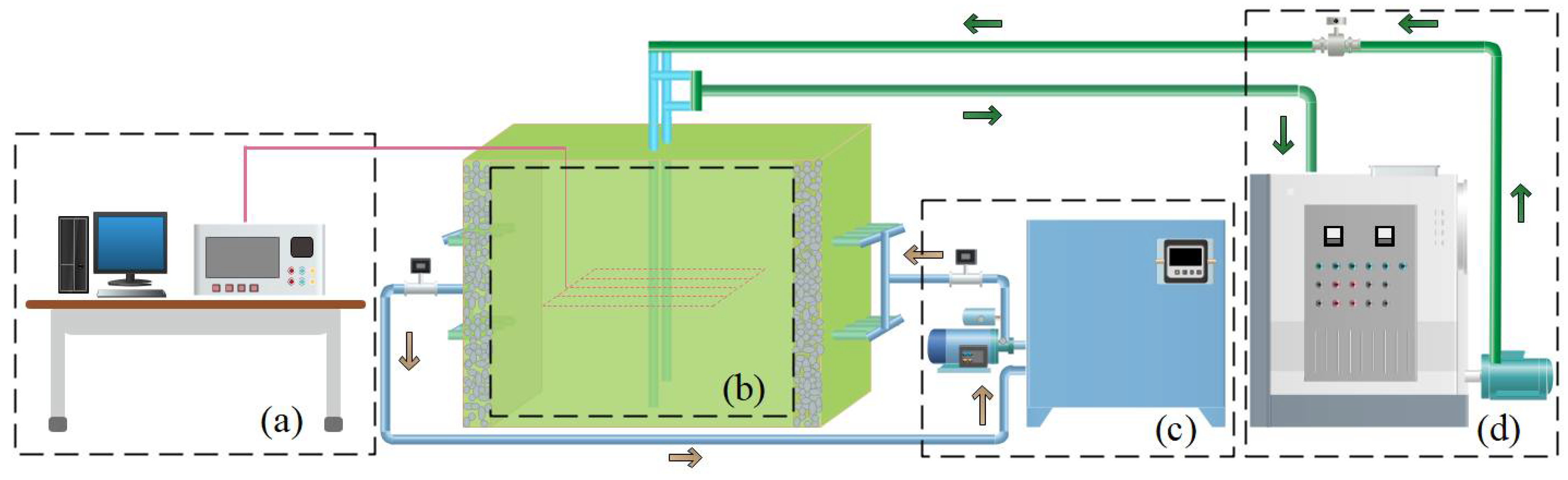
3.2. Design of the Freezing in Saline Sand

The adjustability and accuracy of the velocity and salinity in the model test should be considered in the test design. During the freezing, the key to the model test in saline soil is to form stable velocity conditions and uniform salinity distributions. To ensure the reliability of the test system, a new test system was established based on the mature hydrothermal coupling test system without considering salinity [24]. After the test system was established, 2/3 of the calculated amount of NaCl salt powder was added into the water tank. Then the constant-temperature brine circulation system was turned on, which was maintained at a low velocity for at least 4 h. A salinity meter with an accuracy of 0.01% was used for the continuous measurement until the salt concentration no longer changed. The NaCl powder was added to the tank again, and the previous step was continued. Notably, the closer the measured value is to the target concentration, the lower the amount of salt that should be added. The above steps were repeated until the target salinity was reached. For the freezing test with the velocity of 0 m/d, after the target was reached, the water circulation was closed. In order to ensure that the core test area was in a stable state, the freezing test can only be started after waiting for 12 h. For the freezing test under the velocity of 3 m/d or 6 m/d, during the freezing process, salt will migrate to the freezing front with water. During the freezing process, the salinity in the thermostatic water tank was detected and supplemented when required. In this model test, the test with a low velocity and low salinity was carried out first, and the test with a large velocity and high salinity was carried out last.

The temperature was measured using the TDS630, with a measurement accuracy of 0.1 °C. In the box body, the test plane was arranged at the central height of the box body, and the temperature measuring points were arranged around the frozen pipe on the A–E axis, as shown in Figure 6. There were two freezing pipes on the B and D axes, denoted as the main surface. The C axis is located at the center of the two freezing pipes, denoted as the interface. The temperature changes in the saline sand layer were monitored in real time through 65 temperature measuring points located upstream and downstream. Outside the box, the ambient temperature, water temperature, and temperatures of the inlet and outlet of the frozen pipe were measured simultaneously. During the test, the temperature of the water was controlled at 15 °C using the constant-temperature controller. The temperature of the freezing refrigerant was set to −30 °C. Figure 7 shows the measurement results of the inlet and outlet temperatures of the freezing pipe in the test. As shown, the temperatures at the two locations vary synchronously, At the beginning of freezing, the temperatures of the inlet and outlet pipes dropped rapidly and approached −30 °C, and then maintained near −30 °C. The freezing pipe is a casing, and the refrigerant enters from the inner pipe and exits from the outer pipe. The sand layer in the box absorbs the cooling capacity of the freezing pipe and conducts it to the surrounding. The temperature of the refrigerant increases due to the cooling loss, and the increased temperature reflects the amount of energy absorbed by the sand layer. Figure 7 shows that the difference between the inlet and outlet temperatures develops gradually. The temperature difference increases rapidly at the beginning of freezing and reaches the maximum of 1.2 °C at 4 h. In this stage, the temperature difference between the sand layer temperature and the freezing tube temperature is significant, and the degree of heat exchange is high. Subsequently, as the temperature difference between the sand layer and the frozen pipes decreases, there is less heat exchange between the two, and the temperature difference between the inlet and outlet of the frozen tube gradually decreases and finally reaches close to 0 °C.

4. Analysis of Freezing Model Test Results in Saline Sand

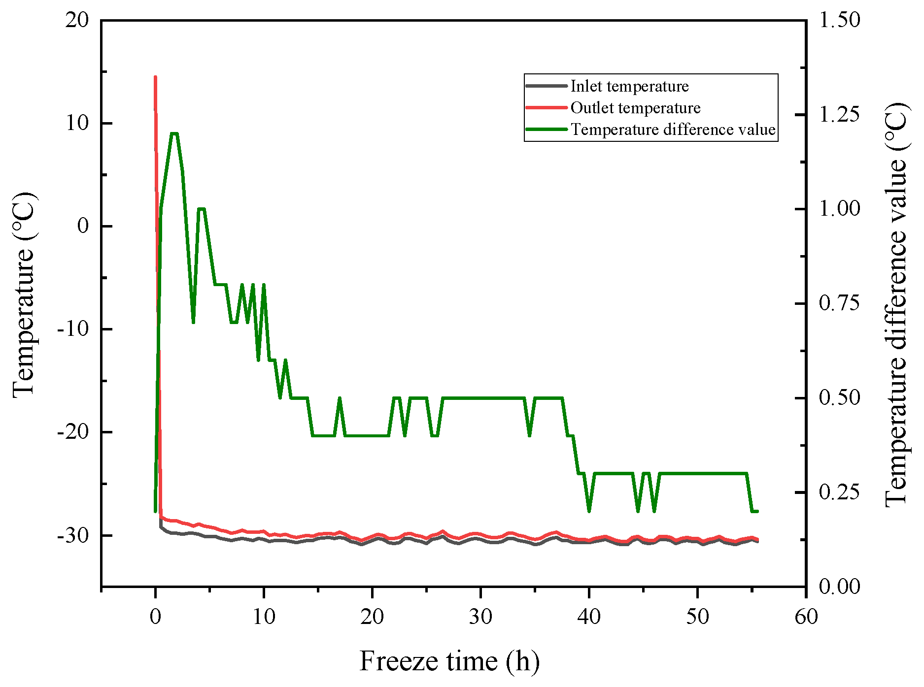
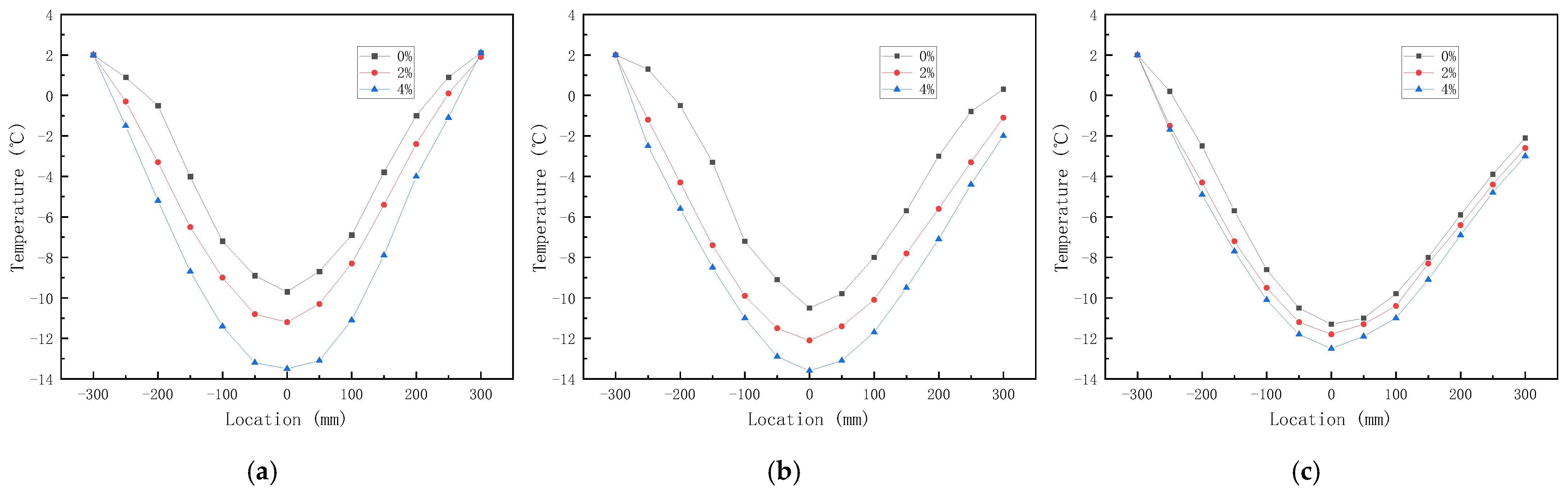
4.1. Temporal and Spatial Development of Freezing Temperature Field in Saline Sand

Based on the test platform, nine groups of double-pipe freezing tests under three velocities and three salinities were carried out according to the above steps. Through the measuring points in the saline sand, the temperature data and temperature spatial distribution at different time under different test conditions were obtained. The spatial distribution characteristics of temperature under different test conditions have been analyzed. Figure 8 shows the temperature field distribution when freezing for 32 h. In Figure 8, low temperature zones were formed centered on the freezing pipes. The temperature distribution was different under different test conditions. Spatially, taking the temperatures at measuring points on the main surface B axis as an example. During the freezing process, the temperature distributions on the B axis were consistent. That is, temperature curve centered on the freezing pipe is formed. The velocity and salinity made the distribution of temperature field different. Figure 9 shows the temperatures on the B axis under different test conditions. It should be mentioned that the temperatures at B1 were all 2 °C for convenient comparisons.

In Figure 9a, the temperature at each measuring point was symmetrical. The temperature at B7 was the lowest, which was about −28.5 °C. Except for the temperatures at B1 and B7, the temperature of each point under different salinities was different. Taking B2 to B6 as an example, the higher the salinity, the lower the temperature at each measuring point. As can be seen from Figure 9a, the higher the salinity, the closer the temperature curve to the linearity. This meant that the temperature on B axis was more well-distributed. The reason for this phenomenon is that the higher the salinity, the smaller the thermal conductivity. When the boundary temperature was the same, the freezing time was longer, which made the temperature developed more fully and evenly. In Figure 9b,c, the temperature distribution was similar to that in Figure 9a. When the temperature at B1 was 2 °C, the higher the salinity, the lower the temperature at each measuring point. However, due to the effect of the velocity, the temperature in the downstream was lower than that in the upstream. The larger the velocity, the larger the temperature difference between the upstream and downstream. The test results showed that under the coupling effect of the velocity and salinity, the temperature difference in the upstream was small, and there was a large temperature difference in the downstream far from the freezing pipe.

The temperature difference between B13 and B1 under nine groups of test conditions could be obtained from Figure 9. The data are summarized in

Table 4. The temperature difference between B13 and B1 under different test conditions.

The Velocity	The Salinity
	0	2%	4%
0 m/d	0	0	0.1
3 m/d	2.1	3.6	4.6
6 m/d	3.6	4.5	5.9

. After ignoring the measurement error, it can be considered that the larger the velocity, and the greater the salinity, the larger the temperature difference. When the velocity was 6 m/d and the salinity was 4%, the maximum temperature difference was 5.9 °C. The temperature difference was approximately linear with the salinity. When the seepage velocity is 3 m/d or 6 m/d, the salinity increases by 1% and the temperature difference increases by about 0.6 °C.

The temperatures on the interface C axis were selected to further analyze the distribution characteristics of the temperature field. the temperature distribution was select for analysis when C1 temperature was 2 °C. Figure 10 shows the temperatures on the C axis under different velocity and salinity conditions. In Figure 10a, the temperature at each point on the C axis was also symmetrically distributed. Since there was no freezing pipe on the C axis, the temperature at each point was higher than the temperature on the B axis. In addition, the temperature difference between the measuring points was also relatively small. Comparing the temperatures under different salinities, the higher the salinity, the lower the temperature at the same location. In connection with the actual project, it can be known that when the same temperature target in a certain area (the temperature in this paper is 2 °C), the higher the salinity, the lower the temperature around the freezing pipe and the lower the average temperature in the area. Under the three salinity conditions, the temperature at C7 was the lowest, which was −9.7, −11.2 and −13.5 °C, respectively. In Figure 10b,c, due to the effect of the velocity, the temperature distribution was no longer symmetrical. At the same time, the higher the salinity, the lower the temperature. It is noted that on the interface C axis, the salinity had a great effect on the temperature. The temperature difference on the interface caused by the salinity was greater than that on the main surface. Compared with 10a–c, the temperature distribution curves were closer with the increase in the velocity. Under velocities of 0 m/d, 3 m/d and 6 m/d conditions, the temperature differences at C7 between 0% and 4% salinity were 3.8, 3.1 and 2.1 °C, respectively. It indicates that the temperature change caused by the salinity decreases when the flow velocity was large. The effects of velocity and salinity on temperature were related.

4.2. The Overlapping Times of the Frozen Curtain under Different Velocities and Salinities

Combined with the temperatures at all measuring points, the development of the frozen curtain can be determined. According to the above research on the saline sand, the freezing temperature of the saline sand was determined. From the above analysis, the freezing temperatures measured for salinities of 0%, 2%, and 4% were −0.1, −1.4, and −3.1 °C, respectively. The temperatures were used as the boundary basis for the frozen curtain. Then the overlapping time of the double-pipe frozen curtain could be obtained. Figure 11 shows the overlapping times under three velocities and three salinities. The existence of salt changed the thermodynamic characteristics of the salinity sand, resulting in the change of overlapping time. In addition, the velocity would also prolong the overlapping time of the frozen curtain. Under the three salinities, the overlapping times increased with the increase in the velocity. But the relationship between the two was nonlinear. Taking 0% salinity as an example, when the velocity increased from 0 m/d to 3 m/d, the overlapping time increased by 24%. When the velocity increased from 3 m/d to 6 m/d, the overlapping time increased by 60%. The overlapping time increased significantly when the velocity was 6 m/d. The relationship between the salinity and overlapping time can be described by a linear function. The slopes of the linear functions under three velocities were 0.88, 1.00 and 1.75, respectively. It showed that the larger the velocity, the greater the effect of the salinity on the overlapping time. Compared the effects of the velocity and salinity on the overlapping time, it is found that the velocity has a great effect on the overlapping time.

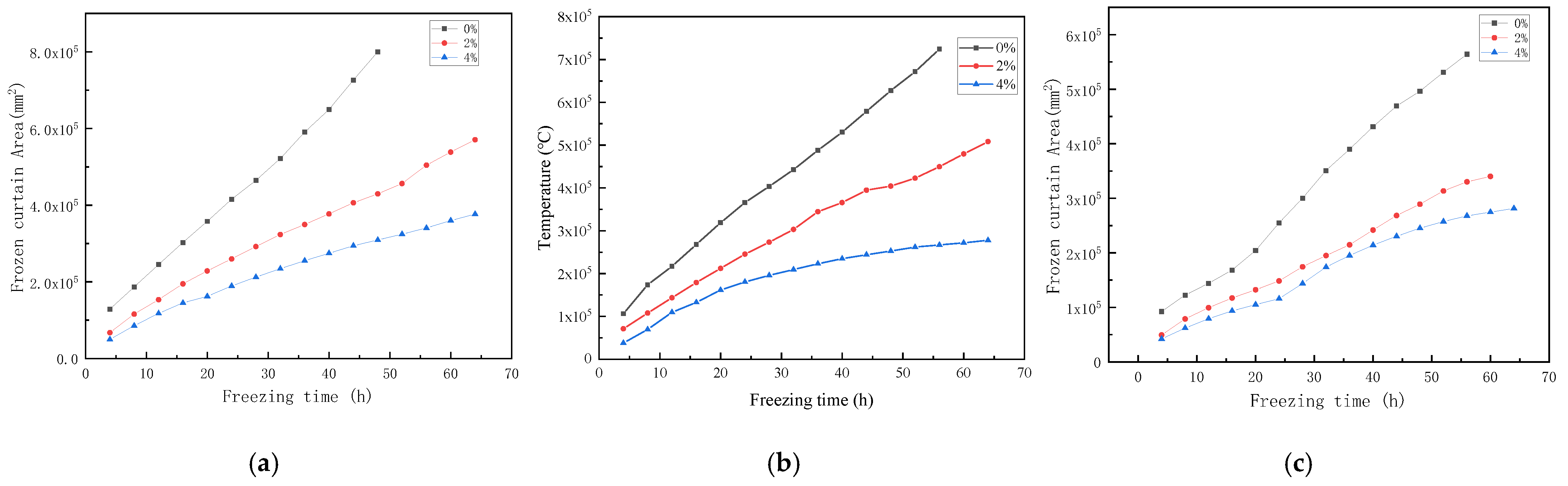
4.3. The Development of the Frozen Curtain under Different Velocities and Salinities

The thickness of the frozen curtain in freezing engineering is worthy of attention. Therefore, the thickness of the frozen curtain was counted. The upstream thickness of the frozen curtain was recorded as R_u and the downstream thickness of the frozen curtain was recorded as R_d. Figure 12 shows the positions of R_u and R_d. According to the temperature at each measured point, the isotherm distribution map was drawn and the outline of freezing temperature was obtained. Figure 13 shows the values of R_u and R_s.

In Figure 13a–c, Due to the different overlapping times, R_u began to develop at different freezing times. At any velocity and any salinity, R_u increased with the freezing time. The development curve of R_u had the same characteristics. R_u increased rapidly in the initial stage of the freezing and the development of R_u gradually slowed down in the later stage of the freezing. At the same velocity and freezing time, the higher the salinity, the smaller the R_u. The salt inhibited the development of R_u. The velocity also had an impact on the development of R_u. The value of R_u when freezing for 48 h is sorted out as shown in

Table 5. The values of R_u when freezing for 48 h (unit: mm).

The Velocity	The Salinity
	0	2%	4%
0 m/d	450	304	227
3 m/d	395	254	196
6 m/d	280	192	175

. Under each salinity, the larger the velocity, the smaller the R_u. Under the conditions of 0% and 4% salinity, when the velocity increased from 0 m/d to 6 m/d, R_u decreased by 38% and 23%, respectively, indicating that the effect of the velocity on R_u was weakened when the salinity was high. Similarly, the effect of the salinity on R_u was weakened at large velocity. It can be found that in the whole process of freezing, the larger the velocity and the higher the salinity, the smaller the R_u.

Figure 14 shows the change of R_d with freezing time. When the velocity was 0 m/d, R_d was the same as R_u. Therefore, when the velocity was 0 m/d, the development of R_d was the same as that in Figure 13a, which was no longer given in Figure 14. However, when the velocity was 3 m/d and 6 m/d, R_d was greater than R_u at the same freezing time. This conclusion is not affected by the salinity. As can be seen from Figure 14a,b, the development laws of R_d and R_u were the same. R_u increased over time, then slowed down and finally stabilized. At the same velocity, the higher the salinity, the smaller the R_d, and with the increase in freezing time, the different became larger and larger. At the same salinity, the greater the velocity, the smaller the R_d. Both the velocity and salinity inhibited the development of R_d.

The frozen curtain area can reflect the development of the freezing. Therefore, the development of the frozen curtain area was obtained in the isotherm diagram. Figure 15 shows the development curves of the frozen curtain. Different from the development law of R_u and R_d, the frozen curtain area kept an approximate linear growth in the freezing process. In Figure 15a–c, the larger the velocity and the higher the salinity, the slower the development of the freezing curtain area. At the same time, when the velocity was large, the difference of the curtain area between different salinities gradually decreased, which indicated that the existence of the velocity decreased the effect of the salinity.

The average development rates of the frozen curtain area during the whole freezing process are shown in

Table 6. The average development rates of frozen curtain area (unit: mm²/h).

The Velocity	The Salinity
	0	2%	4%
0 m/d	15,246	8387	5443
3 m/d	12,366	7284	4116
6 m/d	9434	5191	3987

. It can be found that the average growth rate of the frozen curtain area was affected by the velocity and salinity. The larger the velocity and the greater the salinity, the smaller the development rate. When the seepage velocity was 0 m/d and the salinity was 0%, the development rate was the largest, which was 15246 mm²/h. When the seepage velocity was 6 m/d and the salinity was 4%, the development rate was the smallest, which was 3987 mm²/h. Under the three velocities, when the salinity increased from 0% to 4%, the development rate decreased by 0.64, 0.66 and 0.56. Under the three salinities, when the velocity increased from 0 m/d to 6 m/d, the development rate decreased by 0.38, 0.38 and 0.27. This result indicated that the salinity had a great impact on the development rate of the frozen curtain area.

5. Conclusions

In this research, a double-pipe freezing test platform was established to study the distribution of the temperature field and the development of the frozen curtain in a saline stratum. Double-pipe freezing tests were conducted under three different velocities and salinities. The temporal and spatial distributions of the temperature field and the formation law of the frozen curtain were thoroughly analyzed. From the analysis, the following conclusions can be drawn:

(1) Based on the temperature characteristic curve of the frozen sand, the freezing temperature of the saline sand under different salinities was obtained. The fitting results showed a linear relationship between the freezing temperature and the salinity. When saturated sand was prepared with salt solutions having salinities of 0%, 2%, and 4%, the freezing temperatures of the saline sand were −0.1, −1.3, and −3.1 °C, respectively.

(2) Both the velocity and salinity had a significant influence on the development and distribution of the temperature. The effect of velocity made the temperature in the downstream higher than that in the upstream. The larger the velocity, the greater the temperature difference between the upstream and downstream. When the boundary temperature was the same, the higher the salinity, the lower the temperature. The temperature difference due to the salinity at the interface was greater than that on the main surface. With the increase in the velocity, the effect of salt weakened, and the temperature difference due to the salt decreased gradually.

(3) The analysis of the overlapping time showed that the larger the velocity and the higher the salinity, the longer the overlapping time. The overlapping time increased rapidly with the increase in the velocity. The relationship between the overlapping time and the salinity was approximately linear. Under velocities of 0, 3, and 6 m/d, the growth rates of the overlapping time with the salinity were 0.88, 1.00, and 1.75, respectively. Comparing the effects of the velocity and salinity on the overlapping time, it was found that the velocity had a greater influence.

(4) The upstream thickness R_u and downstream thickness R_d of the frozen curtain increased with the freezing time. Under the effect of the velocity, R_u was smaller than R_d. The velocity and salinity could inhibit the development of the frozen curtain thickness. The effects of the salinity and velocity were coupled and interactive. The area of the frozen curtain increased approximately linearly with the freezing time. Under different test conditions, the development rate of the frozen curtain area was in the range of 3987–15,246 mm²/h. The results showed that the larger the velocity and the higher the salinity, the smaller the development rate of the frozen curtain area. A further analysis showed that salt had a significant influence on the development rate of the frozen curtain area.

References

1. Ministry of Construction, PRC. Code for Geotechnical Engineering Investigation (GB50021-2009); Ministry of Construction: Beijing, China, 2009.
2. Kalinina, N.V.; Rukhovich, D.I.; Pankova, E.I.; Chernousenko, G.I.; Koroleva, P.V. Cartographic analysis of the distribution of saline soils in Russia depending on some climatic parameters. Eurasian Soil Sci. 2016, 49, 1211–1227. [Google Scholar] [CrossRef]
3. Hammam, A.; Mohamed, E. Mapping soil salinity in the East Nile Delta using several methodological approaches of salinity assessment. Egypt J. Remote Sens. Space Sci. 2020, 23, 125–131. [Google Scholar] [CrossRef]
4. Huang, X.; Yao, Z.; Cai, H.; Li, X.; Chen, H. Performance evaluation of coaxial borehole heat exchangers considering ground non-uniformity based on analytical solutions. Int. J. Therm. Sci. 2021, 170, 107162. [Google Scholar] [CrossRef]
5. Zhang, W.; Ma, J.; Tang, L. Experimental study on shear strength characteristics of sulfate saline soil in Ningxia region under long-term freeze-thaw cycles. Cold Reg. Sci. Technol. 2019, 160, 48–57. [Google Scholar] [CrossRef]
6. Korolyuk, T.V. Specific features of the dynamics of salts in salt-affected soils subjected to long-term seasonal freezing in the south Transbaikal region. Eurasian Soil Sci. 2014, 47, 339–352. [Google Scholar] [CrossRef]
7. Li, K.-Q.; Li, D.-Q.; Liu, Y. Meso-scale investigations on the effective thermal conductivity of multi-phase materials using the finite element method. Int. J. Heat Mass Transf. 2020, 151, 119383. [Google Scholar] [CrossRef]
8. Wan, X.S.; Zhang, Q.H.; Xue, M.; Fang, J.H. Road disease and treatment in saline soil area. J. Tongji Univ. 2003, 31, 1178–1182. (In Chinese) [Google Scholar]
9. Bing, H.; Ma, W. Laboratory investigation of the freezing point of saline soil. Cold Reg. Sci. Technol. 2011, 67, 79–88. [Google Scholar] [CrossRef]
10. Wan, X.; Lai, Y.; Wang, C. Experimental Study on the Freezing Temperatures of Saline Silty Soils. Permafr. Periglac. Process. 2015, 26, 175–187. [Google Scholar] [CrossRef]
11. Wu, M.; Zhao, Q.; Jansson, P.-E.; Wu, J.; Tan, X.; Duan, Z.; Wang, K.; Chen, P.; Zheng, M.; Huang, J.; et al. Improved soil hydrological modeling with the implementation of salt-induced freezing point depression in CoupModel: Model calibration and validation. J. Hydrol. 2020, 596, 125693. [Google Scholar] [CrossRef]
12. Xiao, Z.; Lai, Y.; Zhang, M. Study on the freezing temperature of saline soil. Acta Geotech. 2017, 13, 195–205. [Google Scholar] [CrossRef]
13. Zhai, Q.; Ye, W.M.; Rahardjo, H.; Satyanaga, A.; Dai, G.L.; Zhao, X.L. Theoretical method for the estimation of vapour con-ductivity for unsaturated soil. Eng. Geol. 2021, 295, 106447. [Google Scholar] [CrossRef]
14. Zhai, Q.; Rahardjo, H.; Satyanaga, A.; Priono; Dai, G.-L. Role of the pore-size distribution function on water flow in unsaturated soil. J. Zhejiang Univ. A 2019, 20, 10–20. [Google Scholar] [CrossRef]
15. Geng, X.; Boufadel, M.C. Numerical modeling of water flow and salt transport in bare saline soil subjected to evaporation. J. Hydrol. 2015, 524, 427–438. [Google Scholar] [CrossRef]
16. Xu, J.; Lan, W.; Li, Y.; Wang, S.; Cheng, W.-C.; Yao, X. Heat, water and solute transfer in saline loess under uniaxial freezing condition. Comput. Geotech. 2020, 118, 20. [Google Scholar] [CrossRef]
17. Zhang, X.; Wu, Y.; Zhai, E.; Ye, P. Coupling analysis of the heat-water dynamics and frozen depth in a seasonally frozen zone. J. Hydrol. 2020, 593, 125603. [Google Scholar] [CrossRef]
18. Zhang, S.; Wang, Y.; Xiao, F.; Chen, W. Large-Scale Model Testing of High-Speed Railway Subgrade under Freeze-Thaw and Precipitation Conditions. Adv. Civ. Eng. 2019, 2019, 1–14. [Google Scholar] [CrossRef]
19. Ye, C.; Li, Z.C.; Liang, R.Z.; Xiao, M.Z.; Cai, B.H.; Wu, W.B. Analysis of the influence of groundwater salt content on the effect of artificial freezing. Hydro-Sci. Eng. 2021, 2, 78–86. (In Chinese) [Google Scholar]
20. Zhang, T.; Yang, P. Effect of different factors on the freezing temperature of shallow top soil. J. Nanjing For. Univ. 2009, 33, 132–134. (In Chinese) [Google Scholar]
21. Zhou, J.Z.; Tan, L.; Wei, C.F.; Wei, H.Z. Experimental study on freezing temperature and supercooling temperature of soil. Geotech. Mech. 2015, 36, 777–785. (In Chinese) [Google Scholar]
22. Kozlowski, T. Some factors affecting supercooling and the equilibrium freezing point in soil–water systems. Cold Reg. Sci. Technol. 2009, 59, 25–33. [Google Scholar] [CrossRef]
23. Sun, S.C.; Rong, C.X.; Chen, H.; Wang, B. Experimental Study of the Space-Time Effect of a Double-Pipe Frozen Curtain For-mation with Different Groundwater Velocities. Energies 2021, 14, 17. [Google Scholar]
24. Li, Z.X. Research of Salt Migration Rule in Saline Soil; Hefei University of Technology: Hefei, China, 2012. [Google Scholar]
25. Su, W.D. Application of freezing method in the construction of subway connecting aisle under the enriched seawater stratum. J. Water Resour. Archit. Eng. 2019, 17, 181–186. (In Chinese) [Google Scholar]
26. Wang, B.; Rong, C.; Cheng, H.; Cai, H.; Dong, Y.; Yang, F. Temporal and spatial evolution of temperature field of single freezing pipe in large velocity infiltration configuration. Cold Reg. Sci. Technol. 2020, 175, 5902184. [Google Scholar] [CrossRef]
Figure 1. Typical cooling curve of the frozen soil.
Energies 15 01308 g001
Figure 2. Test system and test procedure.
Energies 15 01308 g002
Figure 3. Cooling curve of sand under (a) 0%, 2%, 4%, 6%; (b) 1%, 3%, 5%, 7%.
Energies 15 01308 g003
Figure 4. Variation in the freezing temperature with the salinity.
Energies 15 01308 g004
Figure 5. Freezing model test system (a) temperature acquisition and analysis system; (b) core test area; (c) constant-temperature brine circulation system; (d) freezing circulation system.
Energies 15 01308 g005
Figure 6. The relative position of temperature measuring points to the freezing pipes.
Energies 15 01308 g006
Figure 7. Freezing pipe inlet and outlet temperatures and temperature difference.
Energies 15 01308 g007
Figure 8. The temperature distribution of freezing for 32 h under different test conditions.
Energies 15 01308 g008
Figure 9. The temperature distribution on the main plane D-axis at (a) 0m/d; (b) 3m/d; (c) 6m/d.
Energies 15 01308 g009
Figure 10. The temperature distribution on the interface C-axis at (a) 0 m/d; (b) 3 m/d; (c) 6 m/d.
Energies 15 01308 g010
Figure 11. The overlapping time of double-pipe freezing.
Energies 15 01308 g011
Figure 12. The positions of Ru and Rd.
Energies 15 01308 g012
Figure 13. The developments of Ru at (a) 0 m/d; (b) 3 m/d; (c) 6 m/d.
Energies 15 01308 g013
Figure 14. The developments of Rd at (a) 3 m/d; (b) 6 m/d.
Energies 15 01308 g014
Figure 15. The relation between freezing curtain area and freezing time at (a) 0 m/d; (b) 3 m/d; (c) 6 m/d.
Energies 15 01308 g015