Article

A Parameter Estimation Method for a Photovoltaic Power Generation System Based on a Two-Diode Model

1
Department of Electrical Engineering, Kun Shan University, Tainan 710, Taiwan
2
Department of Green Energy Technology Research Center, Kun Shan University, Tainan 710, Taiwan
*
Author to whom correspondence should be addressed.
Energies 2022, 15(4), 1460; https://doi.org/10.3390/en15041460
Submission received: 23 January 2022 / Revised: 13 February 2022 / Accepted: 14 February 2022 / Published: 16 February 2022

Abstract

:
This study presents a parameter estimation method that uses an enhanced gray wolf optimizer (EGWO) to optimize the parameters for a two-diode photovoltaic (PV) power generation system. The proposed method consists of three stages. The first stage converts seven parameters for the two-diode model into 17 parameters for different environmental conditions, which provides more precise parameter estimation for the PV model. A PV power generation model is then established to represent the nonlinear relationship between inputs and outputs. The second stage involves a parameter sensitivity analysis and uses the overall effect method to remove the parameters that have smaller effect on the output. The final stage uses an enhanced GWO that is associated with measurement data to optimally estimate the parameters that are selected in the second stage. When the parameters are estimated, the predicted value for the PV power output is calculated for specific values of solar irradiation and module temperature. The proposed method is verified on a 200 kWp PV power generation system. To confirm the feasibility of the proposed method, the parameter estimation before and after optimization are compared, and these results are compared with other optimization algorithms, as well as those for a single-diode PV model.

1. Introduction

Photovoltaic (PV) power output is changeable and unpredictable, since it is only generated during the day and not at night. For a large power grid, PV power generation is an uncontrollable power source, therefore there is restricted dispatching. However, the power output from a PV has less inertia than that from traditional units. When an accident occurs in the system, the frequency response decreases as there is a decrease in the inertia of the system, which becomes unstable. Accurately estimating PV power output gives an accurate reference for auxiliary services, such as frequency modulation and rapid response of backup capacity, but the random nature of the output makes estimation difficult.
Estimating parameters for PV power generation involves statistical methods and physical methods. Statistical methods use a black-box model to establish a nonlinear relationship between inputs and outputs. The inputs that are used are the historical PV power output, irradiance, and weather information, and the output is the estimated value for PV power generation. This method uses either indirect or direct forecasting. Indirect prediction [1,2,3] predicts future irradiance using historical irradiance data and other weather variables, and uses a conversion formula to convert irradiance into PV power output. The curves for irradiance and PV power output are quite similar, thus this method usually accurately estimates PV power output if the irradiance prediction is accurate. Direct prediction [4,5,6,7,8,9,10] uses the historical PV power output and weather variables (including irradiance) as input variables, and the prediction results for PV power generation are the output. This method requires an accurate weather forecast to produce good forecast results.
Physical methods establish a physical model for PV power generation between the input and output to convert environmental variables, such as irradiance and temperature, into a power output. Physical model involves either an ideal model [11], a simple power model [12], an experimental model [13], a single-diode model [14,15,16,17,18,19,20,21,22,23,24], a two-diode model [22,23,24,25,26,27], or a three-diode model [28,29]. The single-diode model with five parameters has a simpler architecture, and has been widely used to simulate the electrical behavior of solar cells. To produce more accurate estimate, the two-diode model with seven parameters is developed to enhance the simulation performance in low irradiance. The three-diode model adds another diode to improve the defects of the recombination process in two-diode model [28]. However, the addition of a diode makes the model more complicated. Considering the accuracy and complexity, this study uses a two-diode model to simulate the electrical behavior of solar cells. When the PV power generation model is created, it is difficult to estimate parameters because there is a nonlinear relationship between these parameters. In addition, after a period of operation, the PV module parameters that are provided by the manufacturer change due to aging and deterioration of the solar cell, therefore these must be corrected.
Some parameters affect the output only slightly and will be eliminated in the parameter selection process. When the parameters that affect the output are selected, an optimization tool is used to accurately estimate the parameters. Several optimization algorithms have been used to estimate the parameters of solar cells, such as the hybrid charged system search algorithm [15], the particle swarm optimization (PSO) method [18], the differential evolution algorithm (DE) [19], the chaos-embedded gravitational search algorithm [21], the bonobo optimizer [22], the improved cuckoo search algorithm [23], the chaotic improved artificial bee colony algorithm [24], the ranking-based whale optimizer (WO) [28], and the grasshopper optimization algorithm [29]. As mentioned above, most studies use different optimization tools to solve the parameter estimation problem. The estimation accuracy depends heavily on the chosen optimization algorithm. In addition, the five-parameter and seven-parameter methods, which are respectively used for single-diode and two-diode models, are still imprecise. To solve this problem, a novel approach is proposed in this study. The proposed method consists of three stages. The first stage converts seven parameters for the two-diode model into 17 parameters and establish a PV power generation model in the MATLAB/SIMULINK environment. The second stage combines sensitivity analysis and the overall effect method to remove the parameters that have a smaller effect on the output. The final stage uses an EGWO to optimally estimate the parameters.
The differences compared to the previous studies and the contributions of this study are highlighted as follows:
  • A PV power generation system based on a two-diode model is established in the MATLAB/SIMULINK environment, which can be used for parameter estimation of PV power plants of different types and scales.
  • Converting the seven parameters of the two-diode model into 17 parameters according to different environmental conditions provides more precise parameter estimates for the PV model.
  • A parameter elimination technique that combines parameter sensitivity analysis and the overall effect method is used to remove the parameters that have little effect on the output.
  • To enhance the global search ability of GWO, a dynamic crowding distance (DCD) algorithm is used to eliminate the agents with higher density region in the optimization process.
The remainder of this paper is organized as follows. Section 2 details the PV power generation models. Section 3 describes the proposed parameter estimation method. Section 4 presents the simulation results for a 200 kWp PV power generation system and conclusions are offered in Section V.

2. The PV Power Generation Models

2.1. Single-Diode Model

Figure 1 shows the circuit of a single-diode model which is composed of a photo current source, a diode, a shunt resistance, and a series resistance. The output current of the model is expressed as [14,15]:
I = I L I o e x p V + I R s n I V t 1 V + I R s R s h
where I is the output current for the solar cell, IL is the photo current, Rsh is the parallel resistance, Rs is the series resistance, Io is the saturation currents for the diode, Vt is the thermal voltage, and nI is the ideal factor. Since e x p V + I R s n I V t 1 , Equation (1) can be simplified as [16]:
I = I L I o e x p V + I R s n I V t V + I R s R s h

2.2. Two-Diode Model

For a two-diode model, the saturation current is generated by two diodes. Figure 2 shows the circuit of a two-diode model. The output current for this model is expressed as [25,26,27]:
I = I L I o 1 e x p V + I R s n I 1 V t 1 I o 2 e x p V + I R s n I 2 V t 2 V + I R s R s h
where Io1 and Io2 are the saturation currents for the two diodes, Vt1 and Vt2 are the thermal voltage, and nI1 and nI2 are the ideal factors. In Equation (3), Io2 is used to compensate for the compound loss in the depleted area. This model produces more accurate estimates than a single-diode model if there is low irradiance or shading, but the addition of a diode makes the model more complicated.
Equation (3) shows that seven parameters must be estimated for the two-diode model: IL, Io1, Io2, nI1, nI2, Rs, and Rsh. These parameters change for different irradiance and temperature values as [17,25,26,27]:
I L = G G r e f I L , r e f + α I m p T T r e f
I o 1 = I o 1 , r e f T T r e f 3 e x p q E g k 1 T r e f 1 T
I o 2 = I o 2 , r e f T T r e f 3 2 e x p q E g n I 2 k 1 T r e f 1 T
n I i = n I , r e f ,   i = 1 ,   2
R s = R s , r e f
R s h = R s h , r e f G r e f G
E g = E g , r e f 1 0.0002677 T T r e f
where G is the solar irradiance (kW/m2), Gref is the solar irradiance under standard test condition (STC), T is the surface temperature of the solar cell (K), Tref is the surface temperature under STC, α I m p is the temperature coefficient at the maximum power point, and Eg,ref (eV) is the gap energy for the material under STC. STC defines a test environment with 1000 (W/m2) irradiance, a temperature of 298 (K) and a 1.5 air mass.
Under any environmental conditions, the short-circuit current Isc and the open-circuit voltage Voc are expressed as [17,25,26,27]:
I s c = G G r e f I s c , r e f + α I s c T T r e f
V o c = V o c , r e f + β o c T T r e f
At the maximum power operating point, the current Imp and the voltage Vmp are expressed as [17,25,26,27]:
I m p = I m p , r e f G G r e f
V m p = V m p , r e f + β o c T T r e f
where α I s c is the temperature coefficient at short-circuit current, and β o c is the temperature coefficient at open-circuit voltage.
Combining Equation (4) to Equation (14), the nonlinear relationship between the seven parameters and the related parameters is briefly expressed as:
A Y = B X
where Y = [IL, Io1, Io2, nI1, nI2, Rs, Rsh] and X = [IL,ref, Isc,ref, Voc,ref, Imp,ref, Vmp,ref, Gref, Tref, nI1,ref, nI2,ref, Rs,ref, Rsh,ref, Io1,ref, Io2,ref, αImp, αIsc, β o c , g,ref]. As shown in Equation (14), the seven parameters in Y are controlled by the 17 parameters in X, which are optimized to provide a more accurate estimation of parameters.

3. The Proposed Method

The proposed parameter estimation method establishes a PV power generation model, selects parameters using a sensitivity analysis, and the overall effect method and optimizes parameters using an EGWO. Figure 3 shows a schematic diagram of the proposed method.

3.1. Establishment of PV Power Generation Model

Using the two-diode equivalent circuit, the PV power generation model is established using Matlab/Simulink software. The model inputs are the solar irradiance and the module temperature, and the outputs are the current and power generated. Figure 4 shows the establishment of a PV power generation model, where subsystem1 is used to calculate seven parameters, including IL, Io1, Io2, nI1, nI2, Rs and Rsh, and subsystem2 is used to calculate the current and power output.

3.2. Parameter Selection

To allow more accurate parameter estimation, the original seven parameters in the PV model are converted into 17 parameters for this study. The parameters that are provided by the manufacturer change due to natural degradation of the solar cell. Some parameters have little effect on the output, and can be removed from the model. Parameters are selected to reduce the calculation time for the optimization process.
The parameter selection method for this study uses a parameter-output sensitivity matrix at a specific steady-state operating point. A principal component analysis (PCA) [30] is then used to evaluate the effect on the overall outputs. The magnitude of the parameter effect is evaluated by the sensitivity coefficient S ¯ i j [30]:
S ˜ i j = θ ˜ j y ˜ i y i θ j = θ ˜ j y ˜ i S ¯ i j
where θ ˜ j is the jth parameter, and y ˜ i is the ith output. In Equation (6), j = 1, 2, …, Q, Q is the number of parameters.
There is a disturbance on the jth parameter, such that Δ θ = θ j θ ˜ j , the ith output changes (i.e., Δ y i = y i y ˜ i ) and the sensitivity coefficient is approximated as [30]:
S ¯ i j = y i θ j Δ y i Δ θ j
Equation (17) is a dimensionless sensitivity matrix that expresses the relationship of each parameter with respect to each output. The parameters that have smaller effect on the output are removed in the first step, and the PCA is then used to evaluate the effect of each parameter on the overall outputs.
Combining Equations (16) and (17), the overall effect of the jth parameter is expressed as:
E e f f , j = i = 1 n o λ i P i j i = 1 n o λ i
where E e f f , j   ∈ [0, 1] is the effect of the jth parameter on the overall variables, λ i is the eigenvalue for the ith output, 𝑃𝑖𝑗 represents the degree of contribution for the jth parameter on the ith output, and no is the number of outputs. The parameters with a larger value of E e f f are then optimized using an EGWO algorithm.

3.3. Enhanced Gray Wolf Optimizer (EGWO)

The GWO was proposed by Mirjalili and Lewis [31]. Wolves have very strict social behaviors, which are roughly classified into four categories: α , β , δ , and Ω in order of fitness value. The Ω is the lowest gray wolf, which is dominated by other wolves. The GWO uses surrounding prey, attacking prey, and searching for other prey strategies to model the social behavior of wolves. To enhance the global search ability of GWO, a dynamic crowding distance (DCD) [32] algorithm is used to eliminate the agents with higher density region in the optimization process. Figure 5 shows the pseudocode for the EGWO to optimize the parameters [33], which is described as follows.

3.3.1. Surrounding Prey

The wolves usually use surrounding strategy to hunt prey, which is expressed as [31]:
X t + 1 = X p t A D
D = C X p t X t
where t is the present iteration step, A and C are coefficients, and X and X p denote the location of wolves and the location of the prey, respectively. In Equations (19) and (20), A = 2 a r a and C = 2 r , a decreases linearly from 2 to 0 along the optimization process, and r 0 ,   1 is a random vector.

3.3.2. Attacking Prey

After the surrounding is finished, the wolves stop moving and start attacking their prey. In this stage, Ω wolves change their location based on the best location of α , β , and δ as [31]:
D α = C 1 P α P , D β = C 2 P β P ,   D δ = C 3 P δ P
P 1 = P α A 1 D α , P 2 = P β A 2 D β ,   P 3 = P δ A 3 D δ
P t + 1 = P 1 + P 2 + P 3 3
where P is the location of the wolves, and P α , P β and P δ denote the respective locations of the α , β , and δ wolves.

3.3.3. Search for Other Prey

To achieve a global search, GWO allows A to set randomly greater than 1 or less than −1. This forces an exploratory search and allows the agents to search for the other prey so that the optimization process can run away the local minimum values.

3.3.4. Dynamic Crowding Distance (DCD)

DCD [32] is a diversity maintenance strategy for retaining a certain number of solutions uniformly distributed in the space of feasible solution. In this paper, DCD is employed to eliminate adjacent feasible solutions as follows [32]:
d i = j = 1 , j i C f i t i f i t j f i t m a x f i t m i n
where fiti is the fitness value of the ith feasible agent, fitj is the fitness value of the jth feasible agent, C is the number of feasible agents, and fitmax and fitmin are the maximum and minimum fitness values, respectively.
Equation (24) states that if the value of di is small, the ith feasible agent is in a higher density area and has a higher probability to be eliminated. The deprecated agents will be replaced by randomly generated agents.
In Equation (24), the fitness value is calculated as:
f i t j = j = 1 C O j , e s t O j , m e a 2
Where O j , e s t is the estimated value of the jth agent, and O j , m e a is the measured value of the jth agent. The feasible agent with lower fitness value is better in the iteration process.

4. Numerical Results

The proposed method was tested using a 200 kWp PV power generation system. The data were collected from January 2019 to December 2019, which consists of the hourly historical PV power output and the associated irradiance and module temperature. Due to sunshine, the data in summer season (from June to September) were collected from 06:00 a.m. to 19:00 p.m. at a total of 14 points; in the non-summer season, data were collected at a total of 12 points from 06:00 a.m. to 17:00 p.m. To verify the feasibility of the proposed method, the proposed EGWO was compared with the other swarm optimization algorithms such as PSO and WO. To evaluate the accuracy of the forecast, the mean relative error (MRE) is used as follows [15]:
MRE = 1 N i = 1 N P f o r e P t r u e P c a p × 100 %
where Pfore is the estimated value, Ptrue is the actual value, Pcap is the capacity of the PV power generation, and N is the number of data points. As shown in Equation (26), the MRE is calculated by dividing the estimation error by the capacity of PV power generation in order to reduce the weight of the lower power generation to the error percentage.

4.1. Establishment of PV Power Generation Model

Table 1 indicates the reference values for the 17 parameters under STC. These parameter values are obtained by the manufacturer or by experience. A PV power generation model is then created using the 17 parameters in the MATLAB/SIMULINK environment. Figure 6 shows the current–voltage (I-V) and power–voltage (P-V) characteristic curves for diverse irradiance values. The higher the irradiance, the larger is the output current and power, but the effect on the maximum voltage is small. Figure 7 shows the I–V and P–V curves under different temperatures. The greater the module temperature, the less is the output current and power, and there is a significant effect on the maximum voltage. As observed in Figure 6 and Figure 7, irradiance affects current and power output more than module temperature.

4.2. Parameter Selection for Optimization

To determine the effect of individual parameters on the outputs, a parameter sensitivity analysis with ±5% disturbance is used, and the results are shown in Table 2. The results for the overall effect value show that parameters IL,ref, Voc,ref, Isc,ref, Vmp,ref, Imp,ref, Gref, Tref, Rs,ref, Rsh,ref, nI1,ref,   α I m p , and β o c have a greater effect on the output, parameters Io1,ref, Io2,ref, α I s c , and Eg,ref have little effect on the output. Furthermore, nI2,ref = nI1,ref, therefore nI2,ref can be removed. Obtained from this table that in the optimization process, the five parameters Io1,ref, Io2,ref, α I s c , nI2,ref, and Eg,ref will remain unchanged, and only 12 parameters are used for optimization.

4.3. Parameter Optimization
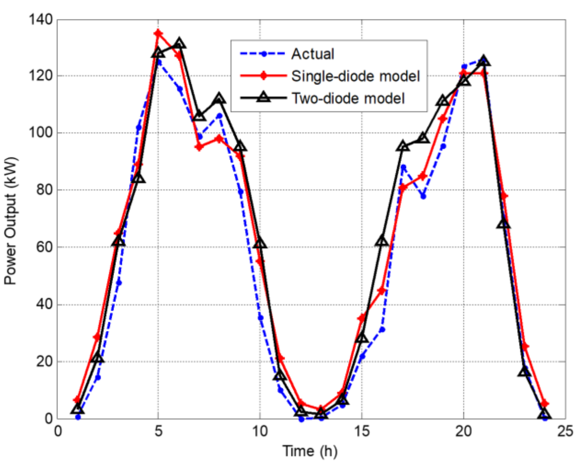
This paper uses an EGWO to optimize the 12 parameters that are selected in the parameter selection stage. Table 3 shows the reference parameters and the parameters after optimization. The ranges for parameters are set in terms of operator experience. In total, four different weather types, including sunny, rainy, cloudy, and slightly cloudy, are used to study the estimation results. Table 4 shows a comparison of the estimation results before and after parameter optimization for different weather types. An optimized parameter gives a smaller value for MRE than one that is not optimized. To verify the performance of the proposed EGWO method, the similar swarm optimization algorithms, such as PSO [18,34] and WO [28,35], are also used to optimize the 12 parameters. The numerical results are shown in Table 5. The proposed EGWO outperforms PSO and WO for different weather types. This table also shows that optimized estimates produce more accurate results than the parameters that are not optimized. The average computation time of the PSO and WO methods through 10 different runs is 12.5 min. and 10.5 min., respectively, while the proposed EGWO takes approximately 9.1 min.
Table 6 shows the estimation results for different PV models using EGWO. The single-diode model with nine parameters produces lower MRE than the single-diode model with five parameters. Similarly, the proposed two-diode model with 12 parameters allows better estimate than the two-diode model with seven parameters. The results in this table show that using Equation (15) to convert the original model to a more refined model according to different environmental conditions can provide more accurate parameter estimation.
Figure 8, Figure 9, Figure 10 and Figure 11 respectively show a comparison of the estimation results for a two-diode model and a single-diode model for sunny, rainy, cloudy, and slightly cloudy days. In total, nine parameters are optimized for the single-diode model, which are selected from the original 13 parameters. The curves show that the two-diode model produces better estimation results than the results for a single-diode model. Table 7 compares the estimation performance of the two models for different time periods. The two-diode model gives better estimation results in the morning and afternoon periods if irradiance is low. The two models give similar results for the higher irradiance period at noon. The average error for the two-diode model shows that it gives better estimation results than the single-diode model.

4.4. Discussion

The following observations are yield from the above results:
  • A photovoltaic power generation system based on a two-diode model is established in the MATLAB/SIMULINK environment, which can be applied to PV power plants of different types and scales only by changing the number of modules in series and parallel.
  • As observed in Table 4 and Table 5, the proposed algorithm combining GWO and DCD allows better global search ability and lower estimation error than the PSO and WO methods.
  • As shown in Table 6, whether a single-diode model or a two-diode model is used, it is more accurate to convert the original model to a more refined model with more parameters according to different environmental conditions.
  • Although the proposed EGWO takes approximately 9 min to complete the parameter optimization, it only needs to be executed offline, and usually needs to be performed once a month or when a new PV array is installed.

5. Conclusions

This study creates a PV power generation system based on a two-diode model in the MATLAB/SIMULINK environment. A sensitivity analysis and the overall effect are then used to eliminate the parameters that have a smaller effect on the outputs. An enhanced GWO algorithm is employed to optimize the 12 parameters that are selected from the original 17 parameters. Testing on a 200 kWp PV power generation system shows that optimized parameters produce better estimation results than parameters that are not optimized for four different weather types. When compared with PSO and WO algorithms, the proposed EGWO allows for better optimization performance in terms of estimation error and computation time. Whether a single-diode model or a two-diode model is used, it is more accurate to convert the original model to a more refined model with more parameters according to different environmental conditions. Furthermore, a two-diode model gives better estimation results than a single-diode model in the morning and afternoon when irradiance is lower. The two modes give similar results during the high irradiance period at noon. The average error values show that the two-diode model gives better estimation results. Although the proposed method allows more accurate estimate than previous works, the estimation error caused by the shading effect is still unsolved, which is the limitation of the proposed method. A future work to improve the estimation error due to shading is under study. In addition, the weather information, such as wind speed and wind direction, which affect heat dissipation from the PV module, can be considered as input to increase the estimation accuracy.

Author Contributions

This paper is a collaborative work of all authors. Conceptualization, C.-M.H. and S.-J.C.; methodology, C.-M.H.; validation, C.-M.H. and S.-P.Y.; writing—original draft preparation, C.-M.H. All authors have read and agreed to the published version of the manuscript.

Funding

This research was funded by the Ministry of Science and Technology, Taiwan, ROC, under the grants MOST 110-3116-F-006-001.

Institutional Review Board Statement

Not applicable.

Informed Consent Statement

Not applicable.

Data Availability Statement

Not applicable.

Conflicts of Interest

The authors declare no conflict of interest.

Nomenclature

α I m p Temperature coefficient at the maximum power point
α I s c Temperature coefficient for the short-circuit current
β o c Temperature coefficient for the open-circuit voltage
λ i Eigenvalue of the ith output
θ ˜ j The jth parameter
A Coefficient vector
CNumber of feasible agents
C   Coefficient vector
d i Diversity of the ith agent
DCD Dynamic crowding distance
DE Differential evolution
EGWO Enhanced gray wolf optimizer
E e f f , j The effect of the jth parameter with respect to the overall variables
E g Gap energy
E g , r e f Gap energy under STC
f i t i Fitness value of the ith feasible agent
f i t j Fitness value of the jth feasible agent
f i t m a x Maximum fitness value
f i t m i n Minimum fitness value
GSolar irradiance
G r e f Solar irradiance under STC
GWO Gray wolf optimizer
IOutput current
I L Photo current
I L , r e f Photo current under STC
I m p Maximum output current
I m p , r e f Maximum output current under STC
I o   I o 1 ,   I o 2 Saturation current
I o 1 , r e f   I o 2 , r e f Saturation current under STC
I s c Short-circuit current
I s c , r e f Short-circuit current under STC
kBoltzmann constant ( 1.38 × 10 23   J / K )
n I   n I 1 ,   n I 2 Ideal factor
n I 1 , r e f   n I 2 , r e f Ideal factor under STC
noNumber of outputs
NNumber of data points
O j , e s t Estimated value of the jth agent
O j , m e a Measured value of the jth agent
P c a p Capacity of the PV power generation
P f o r e Estimated value
P t r u e Actual value
PSO Particle swarm optimization
PV Photovoltaic
P Location of the gray wolf
𝑃𝑖𝑗Principal component element for the jth parameter of the ith output
P α Positions of α wolf
P β Positions of β wolf
P δ Positions of δ wolf
Q Number of the parameter
qElectron charge 1.60 × 10 19   C
R s Series resistance
R s , r e f Series resistance under STC
R s h Parallel resistance
R s h , r e f Parallel resistance under STC
S ¯ i j Sensitivity coefficient in the steady state
S T C Standard test condition
tCurrent iteration
T Surface temperature
T r e f Surface temperature under STC
V Output voltage
V m p   Maximum output voltage
V m p , r e f   Maximum output voltage under STC
V o c   Open-circuit voltage
V o c , r e f   Open-circuit voltage under STC
V t   V t 1 , V t 2 Thermal voltage
WO Whale optimizer
X Location vector of agent
X p   Location vector of the prey
y ˜ i The ith output

References

  1. Liu, J.; Fang, W.; Zhang, X.; Yang, C. An Improved Photovoltaic Power Forecasting Model with the Assistance of Aerosol Index Data. IEEE Trans. Sustain. Energy 2015, 6, 434–442. [Google Scholar] [CrossRef]
  2. Wang, F.; Yu, Y.; Zhang, Z.; Li, J.; Zhen, Z.; Li, K. Wavelet Decomposition and Convolutional LSTM Networks Based Improved Deep Learning Model for Solar Irradiance Forecasting. Appl. Sci. 2018, 8, 1286. [Google Scholar] [CrossRef] [Green Version]
  3. Ramli, A.M.; Makbui, B.; Houssem, R.E.H. Estimation of Solar Radiation on PV Panel Surface with Optimum Tilt Angle Using Vortex Search Algorithm. IET Renew. Power Gener. 2018, 12, 1138–1145. [Google Scholar] [CrossRef]
  4. Sun, Y.; Szucs, G.; Brandt, A.R. Solar PV Output Prediction from Video Streams Using Convolutional Neural Networks. Energy Environ. Sci. 2018, 11, 1811–1818. [Google Scholar] [CrossRef]
  5. Zang, H.; Cheng, L.; Ding, T.; Cheung, K.W.; Liang, Z.; Wei, Z.; Sun, G. Hybrid Method for Short-Term Photovoltaic Power Forecasting Based on Deep Convolutional Neural Network. IET Gener. Transm. Distrib. 2018, 12, 4557–4567. [Google Scholar] [CrossRef]
  6. Zhang, X.; Li, Y.; Lu, S.; Hamann, H.F.; Hodge, B.M.; Lehman, B. A Solar Time Based Analog Ensemble Method for Regional Solar Power Forecasting. IEEE Trans. Sustain. Energy 2019, 10, 268–279. [Google Scholar] [CrossRef]
  7. Lee, W.; Kim, K.; Park, J.; Kim, J.; Kim, Y. Forecasting Solar Power Using Long-Short Term Memory and Convolutional Neural Networks. IEEE Access 2018, 6, 73068–73080. [Google Scholar] [CrossRef]
  8. Agoua, X.G.; Girard, R.; Kariniotakis, G. Probabilistic Models for Spatio-Temporal Photovoltaic Power Forecasting. IEEE Trans. Sustain. Energy 2019, 10, 780–789. [Google Scholar] [CrossRef] [Green Version]
  9. Aprillia, H.; Yang, H.T.; Huang, C.M. Short-Term PV Power Forecasting Using a Convolutional Neural Network-Salp Swarm Algorithm. Energies 2020, 13, 1879. [Google Scholar] [CrossRef]
  10. Lateko, H.; Yang, H.T.; Huang, C.M.; Aprillia, H.; Hsu, C.Y.; Zhong, J.L.; Phuong, N.H. Stacking Ensemble Method with the RNN Meta-Learner for Short-Term PV Power Forecasting. Energies 2021, 14, 4733. [Google Scholar] [CrossRef]
  11. Pavan, A.M.; Mellit, A.; Lughi, V. Explicit Empirical Model for General Photovoltaic Devices: Experimental Validation at Maximum Power Point. Sol. Energy 2014, 101, 105–116. [Google Scholar] [CrossRef]
  12. Mattei, M.; Notton, G.; Cristofari, C.; Muselli, M.; Poggi, P. Calculation of the Polycrystalline PV Module Temperature Using a Simple Method of Energy Balance. Renew. Energy 2006, 31, 553–567. [Google Scholar] [CrossRef]
  13. Jadli, U.; Thakur, P.; Shukla, R.D. A New Parameter Estimation Method of Solar Photovoltaic. IEEE J. Photovolt. 2018, 8, 239–247. [Google Scholar] [CrossRef]
  14. Sabudin, S.N.M.; Jamil, N.M. Parameter Estimation in Mathematical Modeling for Photovoltaic Panel. Mater. Sci. Eng. 2019, 536, 1–11. [Google Scholar]
  15. Huang, Y.C.; Huang, C.M.; Chen, S.J.; Yang, S.P. Optimization of Module Parameters for PV Power Estimation Using a Hybrid Algorithm. IEEE Trans. Sustain. Energy 2020, 11, 2210–2219. [Google Scholar] [CrossRef]
  16. Hou, J.; Xu, P. The Matlab/Simulink Simulation Model of the PV Array Based on the Four-Parameter Model. Renew. Energy Resour. 2013, 31, 10–19. [Google Scholar]
  17. Chouder, A.; Silvestre, S.; Sadaoui, N.; Rahmani, L. Modeling and Simulation of a Grid Connected PV System Based on the Evaluation of Main PV Module Parameters. Simul. Model. Pract. Theory 2012, 20, 46–58. [Google Scholar] [CrossRef]
  18. Ye, M.; Wang, X.; Xu, Y. Parameter extraction of solar cells using particle swarm optimization. J. Appl. Phys. 2009, 105, 094502. [Google Scholar] [CrossRef]
  19. Cárdenas-Bravo, C.; Barraza, R.; Sánchez-Squella, A.; Valdivia-Lefort, P.; Castillo-Burns, F. Estimation of Single-Diode Photovoltaic Model Using the Differential Evolution Algorithm with Adaptive Boundaries. Energies 2021, 14, 3925. [Google Scholar] [CrossRef]
  20. Stornelli, V.; Muttillo, M.; de Rubeis, T.; Nardi, I. A New Simplified Five-Parameter Estimation Method for Single-Diode Model of Photovoltaic Panels. Energies 2019, 12, 4271. [Google Scholar] [CrossRef] [Green Version]
  21. Valdivia-González, A.; Zaldívar, D.; Cuevas, E.; Pérez-Cisneros, M.; Fausto, F.; González, A. A Chaos-Embedded Gravitational Search Algorithm for the Identification of Electrical Parameters of Photovoltaic Cells. Energies 2017, 10, 1052. [Google Scholar] [CrossRef] [Green Version]
  22. Al-Shamma’a, A.A.; Omotoso, H.O.; Alturki, F.A.; Farh, H.M.H.; Alkuhayli, A.; Alsharabi, K.; Noman, A.M. Parameter Estimation of Photovoltaic Cell Modules Using Bonobo Optimizer. Energies 2022, 15, 140. [Google Scholar] [CrossRef]
  23. Kang, T.; Yao, J.; Jin, M.; Yang, S.; Duong, T. A Novel Improved Cuckoo Search Algorithm for Parameter Estimation of Photovoltaic (PV) Models. Energies 2018, 11, 1060. [Google Scholar] [CrossRef] [Green Version]
  24. Oliva, D.; Ewees, A.A.; Aziz, M.A.E.; Hassanien, A.E.; Cisneros, M.P. A Chaotic Improved Artificial Bee Colony for Parameter Estimation of Photovoltaic Cells. Energies 2017, 10, 865. [Google Scholar] [CrossRef] [Green Version]
  25. Kurobe, K.I.; Matsunami, H. New Two-Diode Model for Detailed Analysis of Multicrystalline Silicon Solar Cell. Jpn. J. Appl. Phys. 2005, 44, 8314–8322. [Google Scholar] [CrossRef]
  26. Chin, V.J.; Salam, Z.; Ishaque, K. An Accurate and Fast Computational Algorithm for the Two-Diode Model of PV Module Based on Hybrid Method. IEEE Trans. Ind. Electron. 2017, 64, 6212–6222. [Google Scholar] [CrossRef]
  27. Ishaque, K.; Salam, Z.; Taheri, H. Accurate MATLAB Simulink PV System Simulator Based on a Two-Diode Model. J. Electron. 2011, 11, 179–187. [Google Scholar] [CrossRef] [Green Version]
  28. Mohamed, A.B.; Reda, M.; Attia, E.F.; Sameh, S.A.; Mohamed, A. Efficient Ranking-Based Whale Optimizer for Parameter Extraction of Three-Diode Photovoltaic Model: Analysis and Validations. Energies 2021, 14, 3729. [Google Scholar]
  29. Elazab, O.S.; Hasanien, H.M.; Alsaidan, I.; Abdelaziz, A.Y.; Muyeen, S.M. Parameter Estimation of Three Diode Photovoltaic Model Using Grasshopper Optimization Algorithm. Energies 2020, 13, 497. [Google Scholar] [CrossRef] [Green Version]
  30. Dunteman, G.H. Principal Components Analysis; Sage: Newbury Park, CA, USA, 1989. [Google Scholar]
  31. Mirjalili, S.; Mirjalili, S.M.; Lewis, A. Grey Wolf Optimizer. Adv. Eng. Softw. 2014, 69, 46–61. [Google Scholar] [CrossRef] [Green Version]
  32. Luo, B.; Zheng, J.; Wu, X.J. Dynamic crowding distance: A new diversity maintenance strategy for MOEAs. In Proceedings of the 2008 Fourth International Conference on Natural Computation, Jinan, China, 18–20 October 2008; pp. 580–585. [Google Scholar]
  33. Mirjalili, S. Grey Wolf Optimizer (GWO), Version 1.6, 2018. Available online: https://www.mathworks.com/matlabcentral/fileexchange/44974-grey-wolf-optimizer-gwo (accessed on 25 September 2021).
  34. Biswas, P. Particle Swarm Optimization (PSO), Version 1.5.0.2. Available online: https://www.mathworks.com/matlabcentral/leexchange/43541-particle-swarm-optimization-pso (accessed on 8 February 2022).
  35. Mirjalili, S. The Whale Optimization Algorithm, Version 1.0.0.0. Available online: https://www.mathworks.com/matlabcentral/_leexchange/55667-the-whale-optimization-algorithm (accessed on 8 February 2022).
Figure 1. The circuit of a single-diode model.
Energies 15 01460 g001
Figure 2. The circuit of a two-diode model.
Energies 15 01460 g002
Figure 3. The schematic diagram of the proposed method.
Energies 15 01460 g003
Figure 4. Establishment of a PV power generation model.
Energies 15 01460 g004
Figure 5. The pseudocode for the EGWO to optimize the parameters [33].
Energies 15 01460 g005
Figure 6. The (a) I–V and (b) P–V characteristic curves for different irradiance values.
Energies 15 01460 g006
Figure 7. The (a) I–V and (b) P–V characteristic curves for different temperatures.
Energies 15 01460 g007
Figure 8. Estimation results for a sunny day (25–26 July).
Energies 15 01460 g008
Figure 9. Estimation results for a rainy day (8–9 December).
Energies 15 01460 g009
Figure 10. Estimation results for a cloudy day (1–2 November).
Energies 15 01460 g010
Figure 11. Estimation results for a slightly cloudy day (21–22 June).
Energies 15 01460 g011
Table 1. The reference values for related parameters under STC.
NoParameterReference ValueNoParameterReference Value
1IL,ref (A)3.4510Io1,ref (A)1.16 × 10⁻¹⁵
2Voc,ref (V)66.411Io2,ref (A)1.07 × 10⁻¹⁵
3Isc,ref (A)3.6612nI1,ref1.8609
4Vmp,ref (V)52.013nI2,ref1.8609
5Imp,ref (A)3.5114αIsc (A/K)6.81 × 10−4
6Gref (W/m2)100015αImp (A/K)6.50 × 10−4
7Tref (K)29816 β o c (V/K)−0.166
8Rs,ref (Ω)2.408917Eg,ref (eV)1.121
9Rsh,ref (Ω)150
Table 2. Parameter sensitivity matrix and overall effect value for individual parameters for a ±5% disturbance.
No.ParameterPowerCurrentVoltage E e f f
1IL,ref (A)0.62100.03124.2 × 10−60.9532
2Voc,ref (V)0.0010.0020.00980.3440
3Isc,ref (A)−0.120−0.0025−0.00010.8031
4Vmp,ref (V)0.0040.000755.1 × 10−50.4680
5Imp,ref (A)0.0520.0013.2 × 10−50.7865
6Gref (W/m2)−0.194−0.0038−0.00250.9425
7Tref (°K)0.4900.01250.145250.8821
8Rs,ref (Ω)−0.1155−0.02201−0.00000.7971
9Rsh,ref (Ω)0.00151.3 × 10−50.00110.3635
10Io1,ref (A)3.5 × 10−61.2 × 10−64.8 × 10−50.0806
11Io2,ref (A)2.9 × 10−60.6 × 10−61.6 × 10−50.0912
12nI1,ref0.04100.00238.5 × 10−50.3131
13nI2,ref0.04100.00238.5 × 10−50.3131
14 α I s c (A/K)5.1 × 10−61.8 × 10−61.2 × 10−70.0112
15 α I m p (A/K)0.000670.000322.9 × 10−70.2302
16 β o c (V/K)0.000240.00011−9.3 × 10−70.2031
17Eg,ref (eV)5.1 × 10−61.8 × 10−60.8 × 10−50.0633
Table 3. Reference parameters and optimized values using EGWO.
No.ParameterReferenceRangeOptimization
1IL,ref (A)3.453.4~3.53.42
2Voc,ref (V)66.463~6966.35
3Isc,ref (A)3.663.5~5.43.71
4Vmp,ref (V)52.041~5551.62
5Imp,ref (A)3.513.43~3.653.508
6Gref (W/m2)1000950~10501015.3
7Tref (K)298282~310295.6
8Rs,ref (Ω)2.40892.3~2.52.424
9Rsh,ref (Ω)150130~170148
10nI1,ref1.86091.75~1.951.86
11 α I m p (A/K)6.50 × 10−44.50 × 10−4~8.50 × 10−44.93 × 10−4
12 β o c (V/K)−0.166−0.145~−0.185−0.171
Table 4. Estimation results before and after parameter optimization using EGWO.
Weather TypesOptimizationMRE (%)
Sunny dayBefore optimization3.7532
After optimization1.2542
Rainy dayBefore optimization1.1991
After optimization0.6931
Cloudy dayBefore optimization1.7640
After optimization0.9277
Slightly cloudy dayBefore optimization1.9742
After optimization1.7337
Table 5. Estimation results using different optimization algorithm.
Weather TypeMethodMRE (%)
Sunny dayBefore optimization3.7532
PSO [18,34]
WO [28,35]
EGWO [31,33]
1.8321
1.6235
1.2542
Rainy dayBefore optimization1.1991
PSO [18,34]
WO [28,35]
EGWO [31,33]
0.9125
0.9012
0.6931
Cloudy dayBefore optimization1.7640
PSO [18,34]
WO [28,35]
EGWO [31,33]
0.9936
0.9312
0.9277
Slightly cloudy dayBefore optimization1.9742
PSO [18,34]
WO [28,35]
EGWO [31,33]
1.7452
1.7545
1.7337
Table 6. Estimation error (MRE%) for different PV models using EGWO.
Weather TypeSingle-Diode
Model 1
Two-Diode
Model 2
Single-Diode
Model 3
Two-Diode
Model 4
Sunny day
(25–26 July)
2.85212.80112.29511.7487
Rainy day
(8–9 December)
1.89221.89101.79731.7869
Cloudy day
(1–2 November)
2.23242.20252.03901.7340
Slightly cloudy day
(21–22 June)
2.88652.66982.65382.0996
1 Five parameters (IL,Io, nI, Rs, Rsh) are optimized. 2 Seven parameters (IL,Io1, Io2,nI1, nI2, Rs, Rsh) are optimized. 3 9 parameters (IL,ref, Voc,ref, Isc,ref, Vmp,ref, Imp,ref, Gref, Tref, Rs,ref, Rsh,ref) are optimized. 4 12 parameters (IL,ref, Voc,ref, Isc,ref, Vmp,ref, Imp,ref, Gref, Tref, Rs,ref, Rsh,ref, nI1,ref,   α I m p , β o c ) are optimized.
Table 7. Comparison results of single-diode and two-diode models for different time periods.
Weather TypeTime PeriodSingle-Diode Model
MRE (%)
Two-Diode Model
MRE (%)
Sunny day
(25–26 July)
Morning 12.18551.3590
Noon 23.24842.4492
Afternoon 31.42961.3600
Average error2.29511.7487
Rainy day
(8–9 December)
Morning 12.09532.0278
Noon 21.49201.9675
Afternoon 31.80451.3655
Average error1.79731.7869
Cloudy day
(1–2 November)
Morning 12.48801.0525
Noon 22.52132.1633
Afternoon 31.83131.8188
Average error2.03901.7340
Slightly cloudy day
(21–22 June)
Morning 12.34632.0363
Noon 22.66482.9756
Afternoon 32.88881.2744
Average error2.65382.0996
1: Morning: 06:00–09:00 a.m.; 2: Noon: 10:00–15:00 for June–September and 10:00–14:00 for other months; 3: Afternoon: 16:00–19:00 for June–September and 15:00–17:00 for other months.
Publisher’s Note: MDPI stays neutral with regard to jurisdictional claims in published maps and institutional affiliations.

