Comparison of the Gaussian Wind Farm Model with Historical Data of Three Offshore Wind Farms

Abstract

A recent expert elicitation showed that model validation remains one of the largest barriers for commercial wind farm control deployment. The Gaussian-shaped wake deficit model has grown in popularity in wind farm field experiments, yet its validation for larger farms and throughout annual operation remains limited. This article addresses this scientific gap, providing a model comparison of the Gaussian wind farm model with historical data of three offshore wind farms. The energy ratio is used to quantify the model’s accuracy. We assume a fixed turbulence intensity of $I_{\infty }=6\%$ and a standard deviation on the inflow wind direction of ${\sigma }_{wd}=3°$ in our Gaussian model. First, we demonstrate the non-uniqueness issue of $I_{\infty }$ and ${\sigma }_{wd}$, which display a waterbed effect when considering the energy ratios. Second, we show excellent agreement between the Gaussian model and historical data for most wind directions in the Offshore Windpark Egmond aan Zee (OWEZ) and Westermost Rough wind farms (36 and 35 wind turbines, respectively) and wind turbines on the outer edges of the Anholt wind farm (110 turbines). Turbines centrally positioned in the Anholt wind farm show larger model discrepancies, likely due to deep-array effects that are not captured in the model. A second source of discrepancy is hypothesized to be inflow heterogeneity. In future work, the Gaussian wind farm model will be adapted to address those weaknesses.

1. Introduction

The commercial interest in wind farm control is growing substantially. Although one leading wind turbine manufacturer already provides a wake-steering solution to its customers [1], other original equipment manufacturers and wind farm owners have not yet commercialized the concept. However, several leading wind turbine manufacturers and wind farm developers are actively testing or have been involved with wind farm control experiments, such as Envision Energy [2], TransAlta Renewables [3], NextEra Energy [4,5], General Electric (GE) [6], Renewable Energy Systems (RES) [7], and Engie [8]. According to two recent surveys among a mixed group of experts in academia and industry [9,10], the main challenge preventing wide-scale adoption is validation. The success of a field experiment is highly correlated with the accuracy of the wake model used to devise the control strategy. As field experiments in the literature inconsistently show power gains and losses caused by wake steering, the reliability of the wake models leveraged in these experiments comes into question.

Wind farm control algorithms typically rely on an engineering wind farm flow model to perform many computations at a low computational cost to iterate towards an optimal control policy [11]. Engineering wind farm flow models have been compared to historical wind farm data extensively in the literature. Crespo et al. [12] present an early literature review on wake modeling methods, and present various comparisons of engineering models to wind tunnel and field data, showing reasonable agreement with most models for an 8-turbine array. Rados et al. [13] compare six engineering models to historical data of the Vindeby and Bockstigen offshore wind farms, showing significant variability in the model predictions. Machielse et al. [14] compare their in-house engineering model to field data of a onshore array of five 2.5 MW turbines, spaced 3.8 rotor diameters (D) apart. Renkema [15] compare various engineering models to field data of the Prettin wind farm, which is a small site with GE 1.5 MW turbines, and the Colorado Green wind farm with 108 GE 1.5 MW turbines. The power ratio was calculated and the wake losses were quantified. The authors find that the engineering model by Jensen [16] and the eddy viscosity model by Ainslie [17] show the best agreement with the historical data. Barthelmie et al. [18] compare the Wind Analysis and Application Program (WAsP) engineering model to historical data of the Middelgrunden offshore wind farm with 20 Bonus 2 MW wind turbines. Their wind farm flow model is largely derived from the works of Jensen [16] and Katic et al. [19]. The authors find reasonable agreement between the model and the historical data. However, with a turbine spacing of 2.4 D, it is difficult to generalize these findings. Barthelmie et al. [20] compare a variety of wind farm models to the historical data of the Horns Rev offshore wind farm with 80 turbines. They compare the power ratio for various 5–8 turbine arrays. Then, Barthelmie et al. [21] compare various engineering models to historical data of the Nysted wind farm with 72 turbines and the Horns Rev wind farm. The power ratios are compared for various turbine arrays and a generalized wind farm efficiency is calculated and compared. The large-eddy simulation model seems to outperform the engineering models, which may suggest that the wake superposition principle in the engineering models may lead a loss in model accuracy in large offshore wind farms. Beaucage et al. [22] used the same datasets of the Nysted and Horns Rev wind farm to compare against six commercial and research wake models. They look at turbine arrays of 8 and 10 turbines. The authors split the data by unstable, near-neutral, and stable atmospheric conditions and also look at both 5 deg and 30 deg wind direction sectors. The authors find that the Jensen and Eddy Viscosity model work well until 2–3 turbines downstream, and further in the array tend to overestimate wake recovery. Gaumond et al. [23] propose a different way in comparing engineering models to historical data by using a weighted combination of model simulations to deal with wind direction variability and uncertainty. The authors compare three engineering models to historical data of the Horns Rev offshore wind farm. The inclusion of wind direction variability in model simulations significantly improves agreement between the engineering model and historical data. Nygaard [24] compare their Jensen [16]-based model to historical data of 5 large offshore wind farms, being the 51-turbine Walney I wind farm, the 51-turbine Walney II wind farm, the 175-turbine London Array farm, the 111-turbine Anholt farm, and the Nysted wind farm. Their engineering model only deviates significantly from the London Array wind farm and shows good agreement with data of the other four farms. The same author compares the Jensen [16] model to historical data of 10 offshore wind farms in pursuit of model uncertainty quantification in Nygaard [25]. Across the 10 farms, the results suggest an average model uncertainty that is 15% of the wake loss. Tian et al. [26] proposed a new engineering model based on the Jensen [16] model. The authors compare their new model with historical data with 18 0.3 MW turbines of the Sexbierum wind farm, and with a single turbine of the Nibe wind farm. The results show that the new model better agrees with the wake deficit and shape behind a single turbine at various distances downstream, from 2.5 D to 8 D. Walker et al. [27] compare four engineering models to historical data of five wind farms. The authors look at the power ratio for various turbine arrays and narrow wind direction sectors. Additionally, they look at the wind-farm-wide energy yield for various wind directions and wind speeds, and a measure for the AEP. Like most articles in the literature, the authors do not identify specific strengths or weaknesses in the model, but rather provide a high-level insight into each model’s accuracy. The authors find that no model exceeds a maximum wake loss error of 22%, and therefore propose to reduce the commonly assumed uncertainty of 50% to be reduced to 25% in engineering-model-based wind farm energy yield predictions, in agreement with Nygaard [25]. Archer et al. [28] compare six engineering wind farm flow models to historical data of the Lillgrund offshore wind farm with 48 Siemens 2.3 MW turbines, the Anholt offshore wind farm with 111 Siemens 3.6 MW turbines, and the Nørrekær onshore wind farm with 13 Siemens 2.3 MW turbines. These wind farms vary in regular and irregular layouts, and densely to sparsely spaced. Generally, they find that the Jensen [16] model and their own Gaussian-based wake deficit model demonstrate the best agreement with the historical data. The authors consider the model performance for specific, aligned, and near-aligned wind turbine arrays at different wind directions. However, a broader picture of performance over the full wind rose is missing, and certain partial overlap and irregularly spaced situations are not considered. The authors find that the more packed the wind farm is, the less accurate the engineering models are. Furthermore, the engineering models are more likely to underpredict wake depth, perhaps related to the wake superposition approach by Katic et al. [19] that the engineering models rely on. Nygaard and Newcombe [29] compare the Jensen [16] model and a top–down model to dual-Doppler radar measurements of the 35-turbine Westermost Rough offshore wind farm. The results show that strong coastal gradients complicate the comparison study, and the results are inconsistent in whether the models overestimate wake recovery far downstream. Nygaard et al. [30] propose two new engineering models to deal with large wake clusters and wind farm blockage, respectively. The models are compared with historical data of the Westermost Rough wind farm, showing improved performance over the Jensen [16] model, though discrepancies remain. Hamilton et al. [31] compare various engineering wake models to historical data of the Lillgrund offshore wind farm. The authors demonstrated that different analytical models and model choices agree better with historical data in different atmospheric conditions and farm depths. This analysis was limited to a single wind farm with uncommonly close turbine spacing of 3.2 D to 4.3 D. The results generally showed a high accuracy for the first few rows of turbines, after which accuracy gradually dropped with wind farm depth. It must be noted that most of these articles assume the default model parameters in their comparisons. Thus, it remains uncertain if different models would have performed better had they been tuned to historical data prior to the analysis.

More recently, on the topic of wind farm flow control, Fleming et al. [2] performed a wake steering field experiment using a sector-based modification of the Jensen [16] wake deficit model and the wake deflection model by Jiménez et al. [32]. The authors compare the model predictions against field measurements of two-turbine pairs. They generally find reasonable agreement in wake deficit and wake displacement at the downstream turbines. Then, the authors perform a similar field experiment study in Fleming et al. [4,5], but now with a Gaussian-shaped wake model that includes the effect of counter-rotating vortices, the so-called Gaussian-Curl-Hybrid (GCH) model, according to the works of Bastankhah and Porté-Agel [33], Martínez-Tossas et al. [34], and King et al. [35]. The authors again look at two-turbine pairs, where a single upstream turbine is misaligned with the flow to increase the yield of the pair. The results show that the GCH model agrees well with the measurements in terms of the wake loss experienced by waked turbines. The authors also suggest that there is a real need for models to capture a “secondary steering” effect, which is included in the model by the authors. Then, Fleming et al. [7] use the GCH model for another onshore field experiment for wake steering, again looking at two-turbine pairs at 6 D and 8 D distances, while the experimental data shows large uncertainty bounds, the GCH model seems to capture the general wake loss trends well. Ahmad et al. [36] demonstrates a wake steering field campaign in which the optimal yaw setpoints were designed using a Jensen [16]-based model that additionally accounts for turbulence intensity. Evidence that confirms the reliability of this engineering model is not presented. Howland et al. [3] propose a model based on aerodynamic lifting line theory and follows similar assumptions on the Gaussian shape of the wake and the principle of wake superposition. The authors find good agreement between their simplified model and 5 years of historical field measurements from a 6-turbine wind farm. They also find reasonable agreement between the model and field data in wake steering operation, though the results show significantly more deviations than the five years of historical data. van der Hoek et al. [37] demonstrate a field experiment on axial induction control in arrays of 5 and 6 turbines at the Goole Fields onshore wind farm. They compare their in-house FarmFlow engineering model, which is based on a steady-state, three-dimensional, parabolized simplification of the Navier–Stokes equations. Without tuning the model to historical data, the model predictions show reasonable agreement with the measurements. Doekemeijer et al. [6] present a field experiment for wake steering on 2- and 3-turbine pairs at the Sedini onshore wind farm. The authors use the simplified wind farm flow model from Bastankhah and Porté-Agel [33]. They show reasonable agreement between their model and field measurements for the wake locations, yet the wake depth shows significant discrepancies. Bossanyi and Ruisi [38] present a field experiment for axial induction control on the same site as Doekemeijer et al. [6], but a different set of turbines. The authors compare a set of engineering models based on the Ainslie [17] model and the model by Bastankhah and Porté-Agel [33] to historical data of the site. The models all compare fairly equally, though the stability-dependent Ainslie [17] model by the authors shows marginally better agreement with the historical data for daytime and nighttime, though discrepancies remain. Simley et al. [8] use the same GCH model as Fleming et al. [7] for a wake steering field experiment at a commercial wind farm, again looking at two-turbine interactions, now at 4 D spacing. The authors conclude that the simplified model agrees reasonably well with the field measurements.

Reflecting on the literature, it appears that the GCH model by Bastankhah and Porté-Agel [33], Martínez-Tossas et al. [34] and King et al. [35] is the most prevalent engineering model in wake steering field experiments. In non-wake-steering operation, the GCH model falls back to the Gaussian wind farm flow model by Bastankhah and Porté-Agel [33]. This wake deficit model was initially calibrated through wind tunnel measurements in the original article [33], and has since received limited validation in comparison to historical data in the literature. The articles by Fleming et al. [4,5], Doekemeijer et al. [6], Fleming et al. [7], Simley et al. [8] assessed the engineering model’s accuracy in comparison to field data in two- and three-turbine arrays. Archer et al. [28] compare the model to historical data of 3 wind farms, varying in number of turbines from 13 to 111, in regularly and irregularly spaced farms, and in spacing between the turbines from closely spaced at 3.3 D to more regularly spaced at 5 D. Their results show that the Gaussian model by Bastankhah and Porté-Agel [33] generally over-predicts the power production of waked turbines. The authors also show that the model typically is outperformed by the Jensen [16] model and the authors’ own Gaussian wake deficit model. The authors do not explain where the model discrepancies originate from. Finally, Hamilton et al. [31] compare historical data of the densely spaced Lillgrund wind farm to the Gaussian wake deficit model. The authors limit their analysis to steady historical data and remove any measurements during transient atmospheric conditions. The authors find reasonable agreement with the field data, but also find that different wake models and wake superposition models work better for different scenarios.

This article presents several novel contributions to the literature. To this date, no literature exists in which the Gaussian wake deficit model from Bastankhah and Porté-Agel [33] is compared to historical field data with the objective of informing on further model development. Namely, the current literature is either focused on small [4,5,6,7,8] or uncommonly dense wind turbine arrays [31], or only looks at the high-level accuracy of the model [28]. Additionally, the majority of comparisons of engineering models to historical data have been for narrow wind direction sectors or particular scenarios, rather than for the entire annual operation cycle of the farm. Finally, there has been a significant lack of the inclusion of inflow and measurement uncertainty in the validation of engineering models. This article bridges these gaps by comparing the Gaussian wind farm flow model from Bastankhah and Porté-Agel [33] to historical data of three large offshore wind farms. We consider the important effect of wind direction variability following the approach of Gaumond et al. [23] and include in our analysis the transients in the atmosphere, in contrast to Hamilton et al. [31]. Further, the article at hand uses the energy ratio method to identify situations in which the engineering model diverges significantly from the historical data, identifying fundamental aerodynamic effects that may lack in the model. By doing so, we pave a clear path forward for future model development. Additionally, this article represents multiple years of work on the historical data processing, validation methods, and metrics (e.g., the energy ratio) for model validation. The methods are now contained in an open-source repository [39], which is an equally important contribution.

The article is organized as follows: Section 2 presents the three offshore wind farms from which historical data are compared. Section 3 discusses how the raw data are processed. Then, Section 4 explains the energy ratio metric and how it is used both for wind direction calibration and for model validation. Section 5 presents the engineering wind farm flow model in more detail. Section 6 shows the energy ratios for various turbines for each of the three wind farms, demonstrating the model strengths and weaknesses. Finally, the article is concluded in Section 7.

2. Wind Farms and Measurement Campaigns

Historical data of three offshore wind farms are used for validation in this article. Essential information of the three farms is summarized in

Table 1. Essential information for the three offshore wind farms.

Farm Name	Anholt	OWEZ	Westermost Rough
No. of turbines	111	36	35
Rotor diameter, D (m)	120.0	90.0	154.0
Turbine capacity (MW)	3.6	3.0	6.0
Min. turbine spacing (D)	5	7	6

. The farm layouts are shown in Figure 1.

The first and largest of the three wind farms is the Anholt offshore wind farm off the coast of Denmark. It comprises 111 Siemens SWT-3.6-120 wind turbines, each with a rated power of 3.6 MW. Supervisory control and data acquisition (SCADA) data for this wind farm were recorded from January 2013 to June 2015 at 10 min intervals. Wind direction measurements were not recorded; instead, the wind direction at each turbine was assumed to be equal to the nacelle heading in the remainder of the analysis.

The second wind farm is the Windpark Egmond aan Zee (OWEZ) wind farm off the coast of the Netherlands. It consists of 36 Vestas V90 wind turbines, each with a rated power of 3.0 MW. SCADA data for this wind farm were recorded from December 2006 to December 2010 at 10 min intervals. Wind direction measurements were not recorded; instead, the wind direction at each turbine was assumed to be equal to the nacelle heading in the remainder of the analysis.

The third wind farm is the Westermost Rough wind farm off the coast of the United Kingdom. It comprises 35 Siemens wind turbines, each with a rated power of 6.0 MW. SCADA data for this wind farm were recorded from January 2016 to December 2017 at 10 min intervals. Wind direction measurements were not recorded; instead, the wind direction at each turbine was assumed to be equal to the nacelle heading in the remainder of the analysis.

The wind turbines in those farms were operated under normal conditions during data recording. Therefore, wake steering by yaw misalignment cannot be validated with those data sets. Instead, their function is primarily related to the validation of the velocity deficit, recovery, and non-yaw-induced wake displacement (e.g., secondary steering) effects.

3. Data Preprocessing

Historical data often contain measurements that are contaminated by faulty sensors, turbine downtime, or communication issues. The historical data from the three farms in this article are no different in this aspect. Therefore, this section presents how the SCADA data are processed. First, on a sensor level, the sensor-stuck type of faults were filtered for. Second, on a turbine level, data points far from a turbine’s nominal performance curve were classified as outliers and removed. Third, on a farm level, calibration shifts in the nacelle orientation measurement were detected and, for turbines without shifts in nacelle orientation calibration, the nacelle orientations were calibrated to true north. Each processing step is briefly described next.

3.1. Filtering for Self-Flagged Data, Downtime, and Sensor Faults

First, the data are filtered based on a sensor level. Wind farms commonly have a parameter unique to a turbine or farm indicating the operational status of the wind turbine. For example, the data set from the Anholt wind farm contains a parameter defining how long a turbine has been in operation for the measurement period, which by default is 600.0 s. Any data point reporting a value below 599.0 for this parameter was omitted from the data set.

Second, turbine measurements in which the turbine of interest is reporting a negative wind speed or negative power production are removed from the data set. Those turbines may either be offline for maintenance or the wind speed is simply below the turbine’s cut-in wind speed. In the former case, no valuable information can be derived for model validation. In the latter case, in which the wind speed is low, noise is expected to dominate the measurements, and therefore those data points hold little value and can safely be removed.

Third, a common issue in historical data is when a sensor reports the same value for a large number of consecutive measurements. This behavior is highly improbable for sensors measuring physical parameters such as wind direction and wind speed. In this article, for both the measured wind speed and the wind direction, a turbine’s set of measurements was classified as faulty when six consecutive wind speed or wind direction measurements have a standard deviation smaller than 0.001.

Investigating the dependence of flagged data and their time stamps often reveals periods of turbine downtime—for example, for maintenance reasons. Several periods of downtime were identified in the data sets.

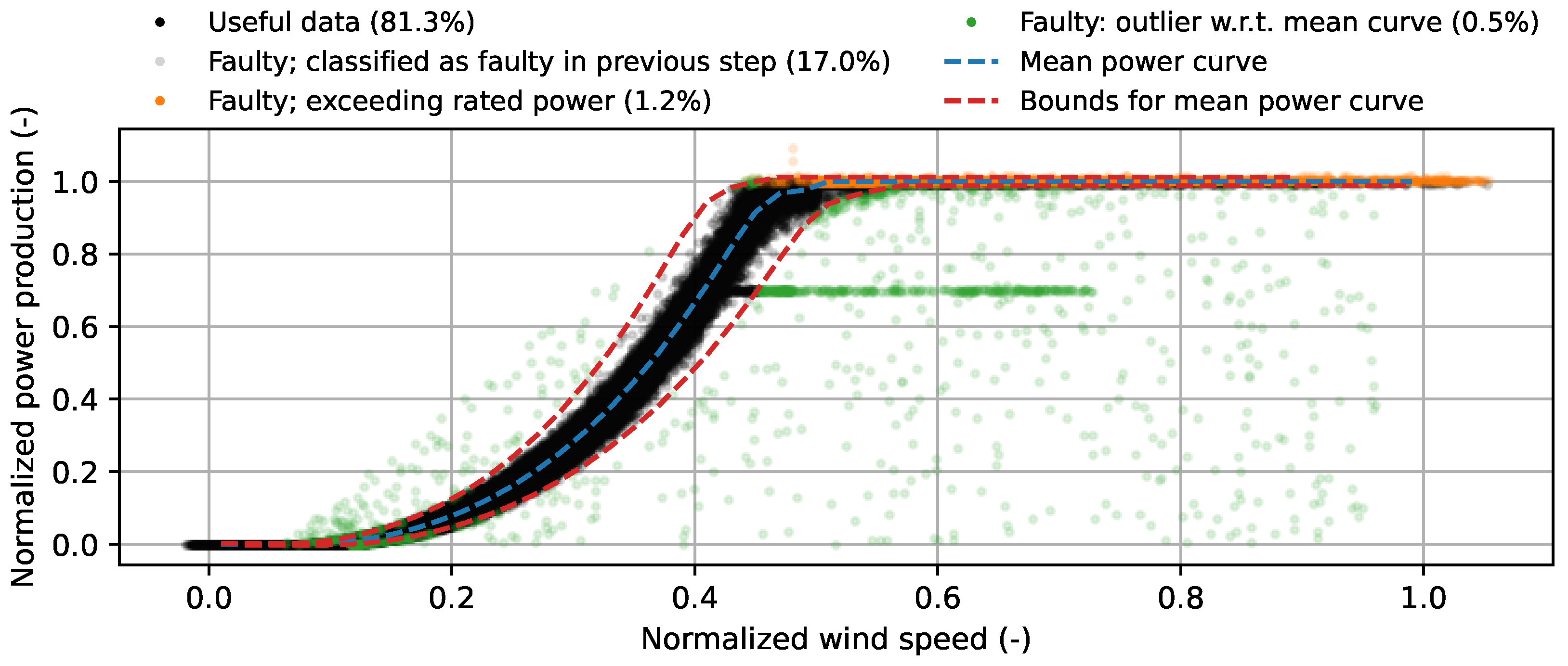
3.2. Filtering for Wind Turbine Performance Curve Outliers

After filtering for faulty sensor readings, the remaining data were filtered by considering individual turbine wind speed and power production measurements. Turbine curtailment is common in historical data and must be addressed before comparing the data with a wind farm model. The general procedure is as follows:

• Data points with a power production more than 5 kW above the rated power were classified as faulty and removed.
• Curtailment periods and other data outliers are removed by iteratively estimating the mean power curve, defined by coordinates $x_{nom}$ (m/s) and $y_{nom}$ (kW), and removing data entries more than a certain distance to the left or right of this curve. The left bound is defined by the curve $x_{lb}=0.92x_{nom}-0.25$ and $y_{lb}=1.01y_{nom}+10.0$. The right bound is defined by the curve $x_{rb}=1.08x_{nom}+0.25$ and $y_{rb}=0.99y_{nom}-10.0$.
• The performance curve was inspected manually to ensure no outliers were missed.

An example of this filtering process is shown in Figure 2.

4. The Energy Ratio as a Calibration and Validation Metric

A common way to compare wind farm models with historical data is through some sort of normalized power deficit. For example, Nygaard [25] defines a loss factor as being the wind farm’s net power production divided by the farm’s gross power production if no wakes were present. The gross power production (without wakes) is extrapolated from the power production of the upstream turbines. However, this metric does not account for individual turbine wake losses, and is therefore insufficient for model validation when that model is to be applied for wind farm control. In this article, the “energy ratio” metric is used.

4.1. The Energy Ratio Defined

In this article, we use a simplification of the energy ratio method as defined by Fleming et al. [4,5]. Essentially, the data are binned along a reference wind direction. The reference wind direction measurements may be derived from one or multiple wind turbines, a lidar, or a meteorological mast. In our case, we derive the wind directions from neighboring turbines. Then, for each bin, the energy ratio for a particular test turbine is calculated as follows:

$$R=\frac{{\sum }_{i=1}^N{\overrightarrow{P}}_i^{\mathrm{test}}}{{\sum }_{i=1}^N{\overrightarrow{P}}_i^{\mathrm{ref}}}.$$

(1)

In this equation, ${\overrightarrow{P}}^{\mathrm{test}}\in {\mathbb{R}}^N$ and ${\overrightarrow{P}}^{\mathrm{ref}}\in {\mathbb{R}}^M$ are vectors of length N, containing the power measurements of the test turbine and the power measurements of the reference turbine(s), respectively. In this article, ${\overrightarrow{P}}^{\mathrm{ref}}$ is defined as the average power production of a set of upstream wind turbines—for example, the five turbines closest to the test turbine or all upstream turbines within a specified radius of the test turbine (e.g., 5 km). This energy ratio metric is equal to the one used in Fleming et al. [4], yet simplified under the condition that each measurement data point contains a valid measurement for both ${\overrightarrow{P}}^{\mathrm{test}}$ and ${\overrightarrow{P}}^{\mathrm{ref}}$.

Physically, R represents the relative power production due to wake impingement (i.e., loss) on the test turbine for a particular wind direction bin. Because measurements at low wind speeds contribute little to R yet are paired with high noise levels, measurements with ambient wind speeds below 6 m/s are excluded in the calculation of R in this article. The ambient wind speed is derived as the average wind speed either from all upstream turbines within a specified radius (typically 5 km) or from a number of closest upstream turbines (e.g., the five closest upstream turbines). Additionally, measurements with ambient wind speeds above 10 m/s are excluded because the power ratio converges to 1.0 the closer the wind speed is to the rated value, which holds little value in model validation.

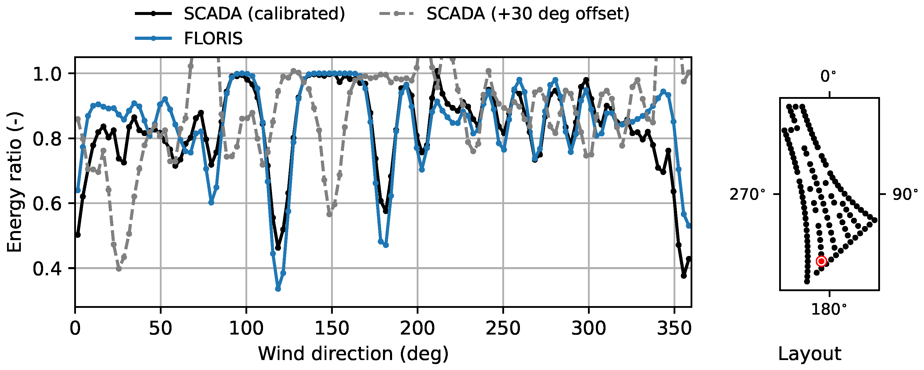
4.2. Calibrating Wind Direction Measurements to True North Using the Energy Ratio

Commercial wind turbines are typically not calibrated to true north, but instead rely on measurements of the relative nacelle misalignment to yaw the turbine into the wind. However, model validation requires the historical data and the model to assume the same zero point and sign convention for the wind direction. Therefore, the wind direction measurements of the turbines are calibrated to true north by comparing the energy ratios for a particular turbine for various corrections on the reference wind direction measurement. The following cost function is optimized:

$$\Delta {\varphi }_{\mathrm{bias}}={arg}_{\Delta \varphi }max\left(\overrightarrow{r}\left({\overrightarrow{R}}^{\mathrm{scada}}\left(\varphi -\Delta \varphi \right),{\overrightarrow{R}}^{\mathrm{model}}\left(\varphi \right)\right)\right),$$

(2)

where $\overrightarrow{r}$ is the Pearson correlation coefficient equaling 1.0 if the two functions are identical. Vectors ${\overrightarrow{R}}^{\mathrm{scada}}$ and ${\overrightarrow{R}}^{\mathrm{model}}$ contain the energy ratios for all wind direction bins for the historical data and for the model predictions, respectively. Note that previous work has followed a simpler but similar method, aligning the wind direction at which the largest wake deficit occurs with the angle between two neighboring turbines. However, the method in this article is more systematic, as it covers the Northing calibration using the entire wind rose, which is more resilient to noisy data. Additionally, this method is able to account for veer and other effects that may be included in the mathematical model.

An example of Equation (2) converging is shown in Figure 3. This figure demonstrates that multiple power losses due to wake interaction can be observed in the data set and can be used for the Northing calibration. Additionally, note that the predicted impact of wakes (FLORIS) is much larger at wind directions of 120° and 180° compared with the historical data (SCADA). Note that this does not necessarily point to a flaw in FLORIS, as is discussed in Section 4.3.

It is important to note that this calibration method fails if the nacelle calibration changes one or multiple times within the data set. Jumps in the nacelle calibration are detected by comparing the average offset between turbine wind direction measurements within the farm. If the average offset between nacelle positions is consistent throughout the entire time series, then both turbines do not experience any jumps in their calibration. However, if this is not the case, then one or both turbines are likely to have experienced changes in their calibration. Iteratively, turbines with inconsistent calibration can be detected and excluded as sources for wind direction measurements. Across the three wind farms, a handful of turbines are found to have an inconsistent calibration. The wind directions of those turbines are therefore to be excluded in model validation and are invalid to use as a reference wind direction for the energy ratios.

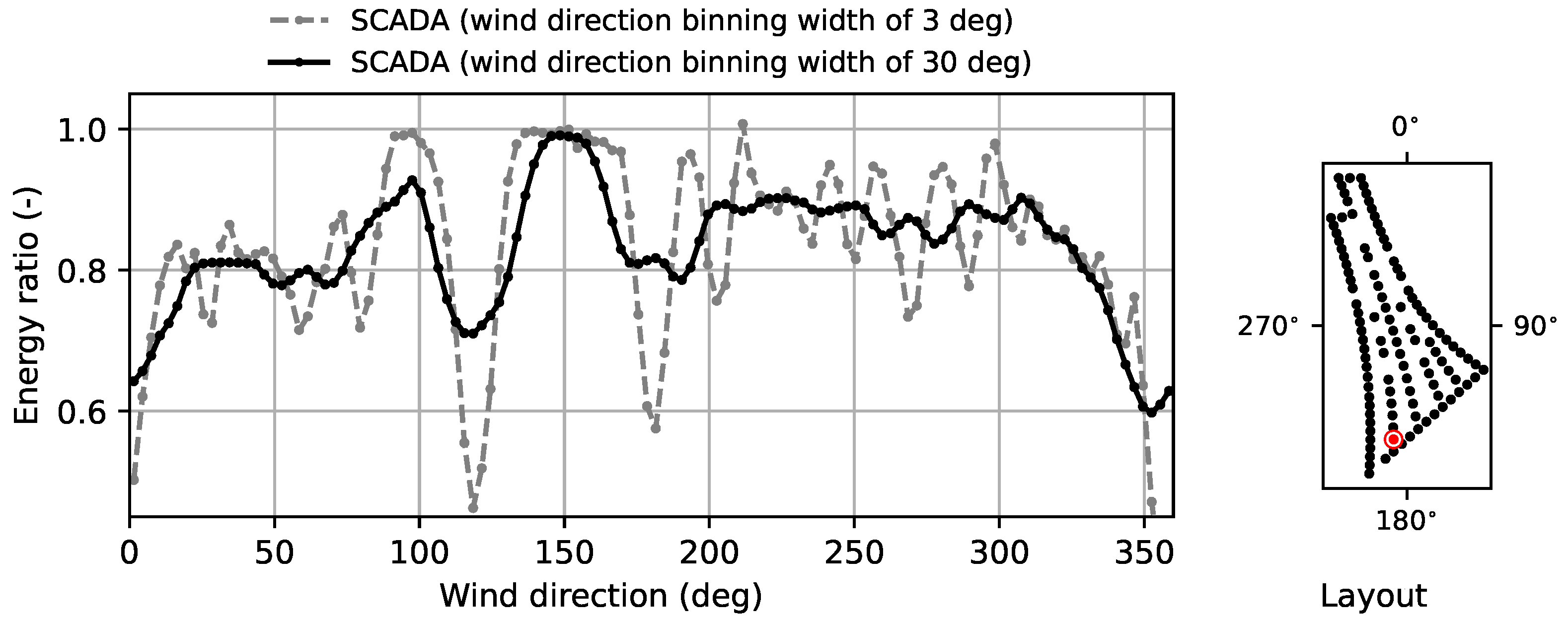
4.3. Binning Choices and Their Relation to Temporal and Spatial Effects in the Wind Farm

The choice of the bin width and bin overlap (data points falling in multiple bins) affects the energy ratio curves in an important manner. Gaumond et al. [23] propose the use of a large bin width of 30° to account for the spatial and temporal wind direction variability and for the slow response time of wind turbine yaw controllers. Because each data point is a 10-minute-averaged representation of a time period, the actual data often would cover multiple bins. Fleming et al. [4] calculated the energy ratio for wind directions from 100° to 180° in steps of 2°, but with bin widths of 4°. They state that introducing overlap between bins (i.e., using wider bins) clarifies trends in the available data, which is in agreement with the findings of Gaumond et al. [23]. An example demonstrating the difference between narrow and wide bins in shown in Figure 4.

A significant difficulty with using large bin widths is that only a broad validation can be made to the wake losses. Separate wake profiles become harder to distinguish, such as for wind directions between 200° and 300° in Figure 4. However, an accurate prediction of the wake deficits and locations is vital for wake steering. Therefore, neither method provides a comprehensive comparison metric; rather, both a small and a large bin width should be considered in model validation.

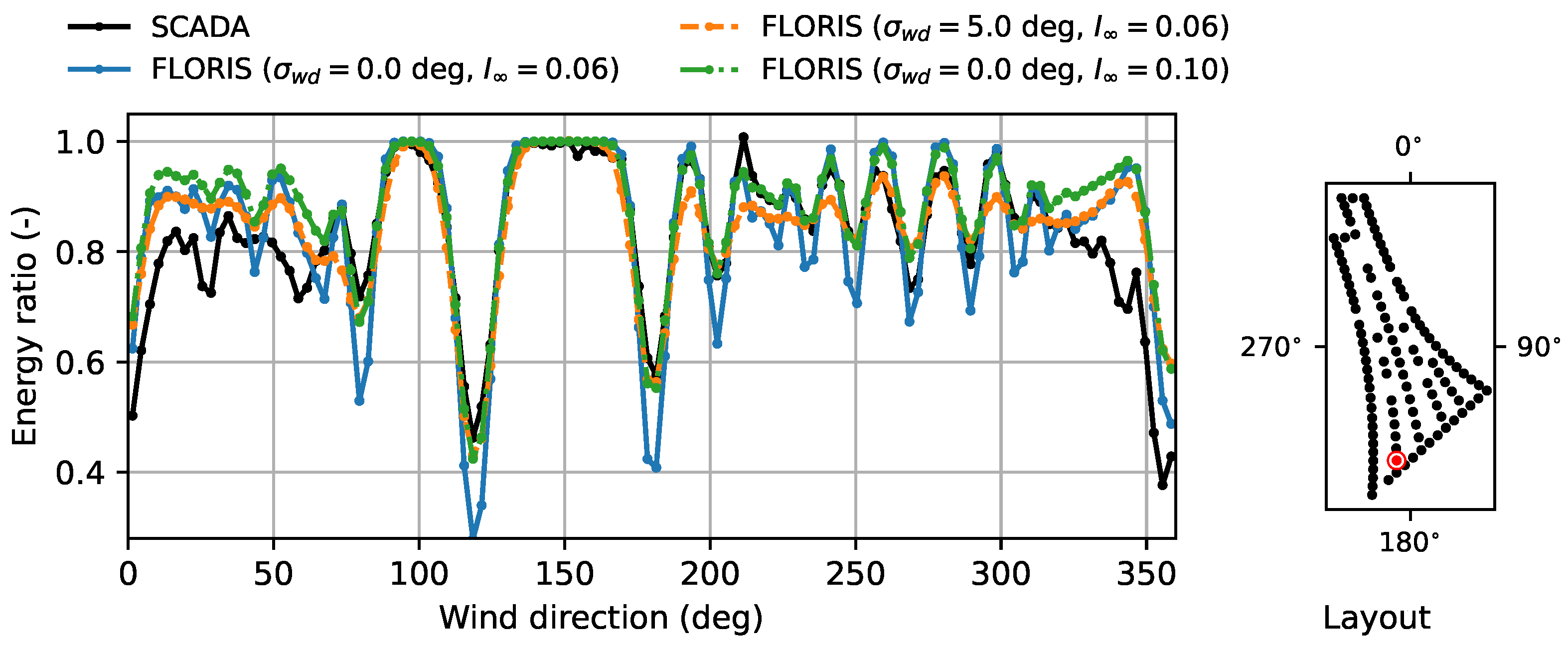
4.4. The Effect of Model Uncertainty, Turbulence Intensity, and Veer on the Energy Ratio

Gaumond et al. [23] also propose using a weighted average of multiple model simulations for each data point to accommodate for the large time constant in the yaw controller, spatial variability of the wind direction inside the farm, and temporal variability of the wind direction within the measurement averaging period of 10 min. Similar solutions to account for yaw and wind direction variability are proposed in the literature [40,41,42], but are mainly focused on wake steering. The choice of turbulence intensity and spatial variability of the wind direction in FLORIS exclusively change the energy ratio of the model-generated data, and do not affect the energy ratios of the SCADA data. Generally, the inclusion of model uncertainty, increasing turbulence intensity, and increasing wind veer have very similar effects: wake effects are smeared out along the wind direction, and the maximum wake deficit decreases.

The effects are demonstrated in Figure 5, where ${\sigma }_{wd}$ is the standard deviation of the incoming wind direction evaluated as described by Simley et al. [42], and $I_{\infty }$ is the ambient turbulence intensity assumed in FLORIS. Figure 5 shows that the wind direction variability ${\sigma }_{wd}$ leads to a smoothing effect of the energy ratios along the wind direction. Turbulence intensity, $I_{\infty }$, has a similar effect but emphasizes the depth of the troughs (largest losses) in the energy ratio curve. The effect of veer has not been tested within FLORIS but fundamentally should further diffuse the wake profile, which should have a similar effect as wind direction variability and turbulence intensity. However, note that veer has a strong correlation with atmospheric stability. Thus, while an increased wind veer diffuses the wake profile, the increased stability in the atmosphere and the lower turbulence intensity it may be paired with could lead to a net increase in wake losses.

Without a clear and common definition for each of those variables, tuning the parameters inside the wake model is ineffectual. The right choice of ${\sigma }_{wd}$, $I_{\infty }$, and wind veer have a deciding impact on the accuracy of the FLORIS model, more than the exact choice of model parameters. Often, those parameters cannot be determined accurately for a commercial wind farm—certainly if no historical data is available for the farm. Additionally, various choices for ${\sigma }_{wd}$ and $I_{\infty }$ can often lead to nearly identical energy ratios, a so-called waterbed effect, making it impossible to identify the right value for each, while different combinations of choices for ${\sigma }_{wd}$ and $I_{\infty }$ can lead to comparable energy ratios, their effect on wake steering differs. Typically, a higher ${\sigma }_{wd}$ with a lower $I_{\infty }$ will predict higher annual energy production gains for wake steering than a low ${\sigma }_{wd}$ and high $I_{\infty }$, despite yielding comparable energy ratios. Hence, selecting those parameters is a nontrivial task. Kanev and Bot [43] make an interesting proposal to linearly correlate the two parameters, while worthwhile to pursue, this is out of our scope and not further explored in this article. Instead, we assume ${\sigma }_{wd}=3.0°$ and $I_{\infty }=0.06$, which are common figures for offshore wind farms in the literature [44,45]. This assumption is the same for the three farms. With the exact definition of those variables being ambiguous and having diverging definitions in the literature, one of the core objectives of the recently initiated International Energy Agency Wind Technology Collaboration Program Task 44 is establishing a common definition [46].

4.5. Uncertainty Quantification

The historical data for the three wind farms was provided as 10 min averages of high-resolution measurements. Additionally, the standard deviation within each 10 min sample set was calculated for the nacelle headings and wind speeds. These may provide some idea of the probability distribution of the quantity of interest, but were not used in the analysis at hand. Additionally, one must keep in mind that the sensors on the turbines are point measurements, and often are affected by the rotor aerodynamics. Hence, there are relatively large bounds of uncertainty on turbine wind speed and vane measurements. In the energy ratio analysis, the main quantities of interest are the turbine nacelle heading and the turbine generator power, which both do not suffer from this sensor disturbance.

To provide quantitative bounds on the uncertainty in the analysis, confidence intervals of 90% on the energy ratio curves are calculated through bootstrapping with a sample size of 100, as described by Efron and Tibshirani [47].

5. Surrogate Modeling

The state-of-the-art wind farm model implemented in FLORIS [48] is used for analysis in this work.

5.1. Model Parameters

The default model parameters were used for the analyses in this article to provide a realistic benchmark situation in which one does not readily have data available for tuning the wind farm model.

Table A1. Parameter and submodel choices in the FLORIS model [48].

Variable	Relates to	Value
velocity_model	Wind speed deficit model	gauss_legacy [33,52]
turbulence_model	Turbulence intensity model	gauss_legacy [33,53]
deflection_model	Wake deflection model	gauss [33,52]
combination_model	Wake combination model	sosfs [19]
use_secondary_steering	Secondary steering model	True [35]
ka	Wake expansion	0.38
kb	Wake expansion	0.004
ad	Lateral wake deflection	0.0
bd	Lateral wake deflection	0.0
alpha	Transition point near-far wake	0.58
beta	Transition point near-far wake	0.077
eps_gain	Value to calculate lateral and vertical flow	0.2
ti_initial	Turbine-induced turbulence [53]	0.1
ti_constant	Turbine-induced turbulence [53]	0.5
ti_ai	Turbine-induced turbulence [53]	0.8
ti_downstream	Turbine-induced turbulence [53]	−0.32

summarizes the parameter choices.

5.2. Heterogeneous Inflow Wind Speed Profile

Commonly, control-oriented wind farm models are simulated with a homogeneous inflow wind direction and wind speed profile. However, in practice, those assumptions are incorrect—wind farms typically experience a lower inflow wind near the center of the farm compared with the outer edges because of wind farm blockage [30]. Additionally, other wind farms and terrain effects upstream can cause different wind conditions for different upstream turbines.

FLORIS currently does not include a blockage or a terrain model. Instead, heterogeneous inflow effects can be directly superimposed in the model by assigning unique wind speeds for each upstream wind turbine. FLORIS supports modeling of heterogeneous inflow conditions for the wind speed, wind direction, and turbulence intensity [49]. Ideally, each measurement in the historical data set would be evaluated in FLORIS with the correct inflow wind speed at every upstream turbine, such that their power productions perfectly match with the SCADA measurements. However, with this many turbines and the inconsistency in data point validity, a generalized inflow profile representative of the farm’s annual inflow heterogeneity is derived.

The heterogeneous inflow profiles are derived from the SCADA data by considering the energy ratios of every upstream wind turbine relative to the average energy ratio of all the upstream turbines for a narrow wind direction sector. The inflow profile for the Anholt wind farm at a wind direction sector of 262.5° through 277.5° is displayed in Figure 6. Figure 6 highlights that significant heterogeneity is present in the inflow of the Anholt wind farm. Note that winds from the west and southwest come from the Danish coast, which may explain some of the inflow heterogeneity. Additionally, blockage effects are expected in Anholt because of the wind farm size. However, without further investigation, the degree to which the coastal effects bring about these heterogeneous inflows and the exact causes of the heterogeneous inflows remain uncertain.

Similar heterogeneity was observed in the OWEZ and Westermost Rough wind farms. Notably, significant heterogeneity is found in the Westermost Rough wind farm for winds from the south and west, as exemplified in Figure 7. This aligns with the relative position of the English coast.

The relative energy ratios of the upstream turbines are calculated in steps of 2° with bin widths of 15°. Those ratios are converted into relative ambient wind speeds by taking the cubic root. Those values are multiplied by the mean wind speed to generate the heterogeneous inflow wind speed profile inserted into FLORIS.

6. Results

This section presents the energy ratio curves, after data preprocessing and the Northing calibration, for various test turbines in the three offshore wind farms.

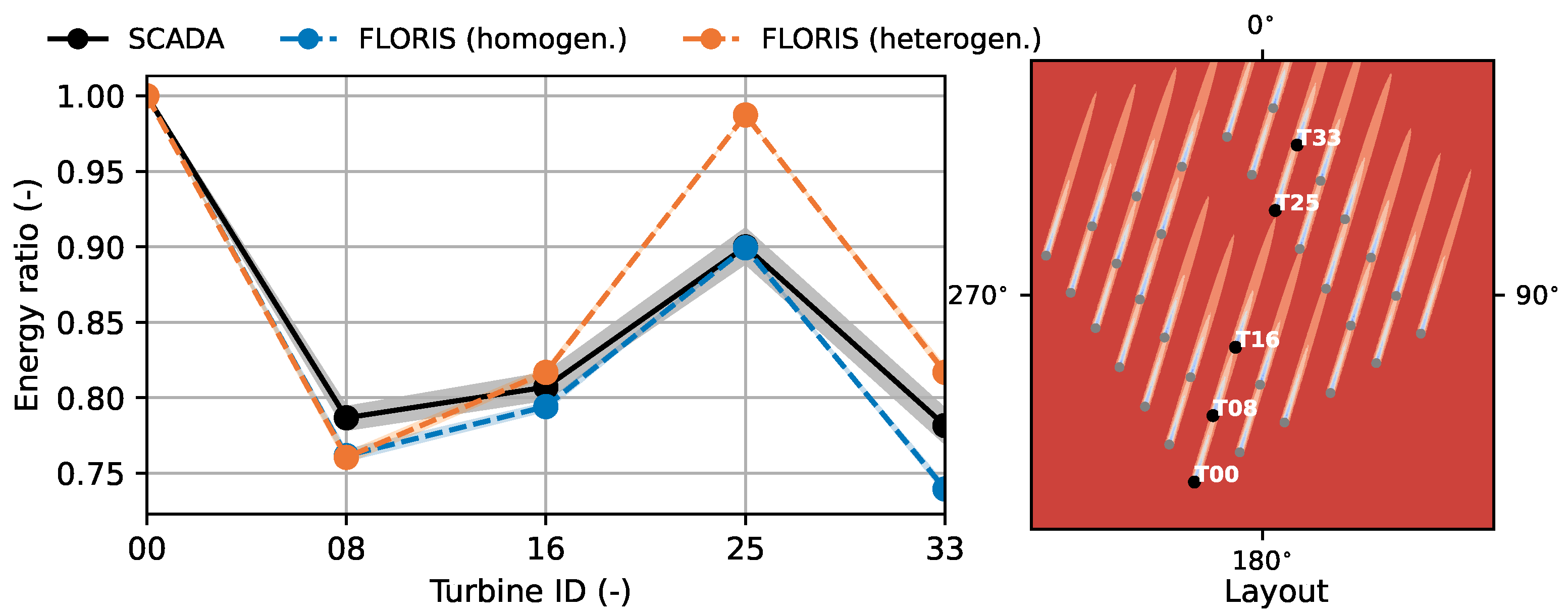
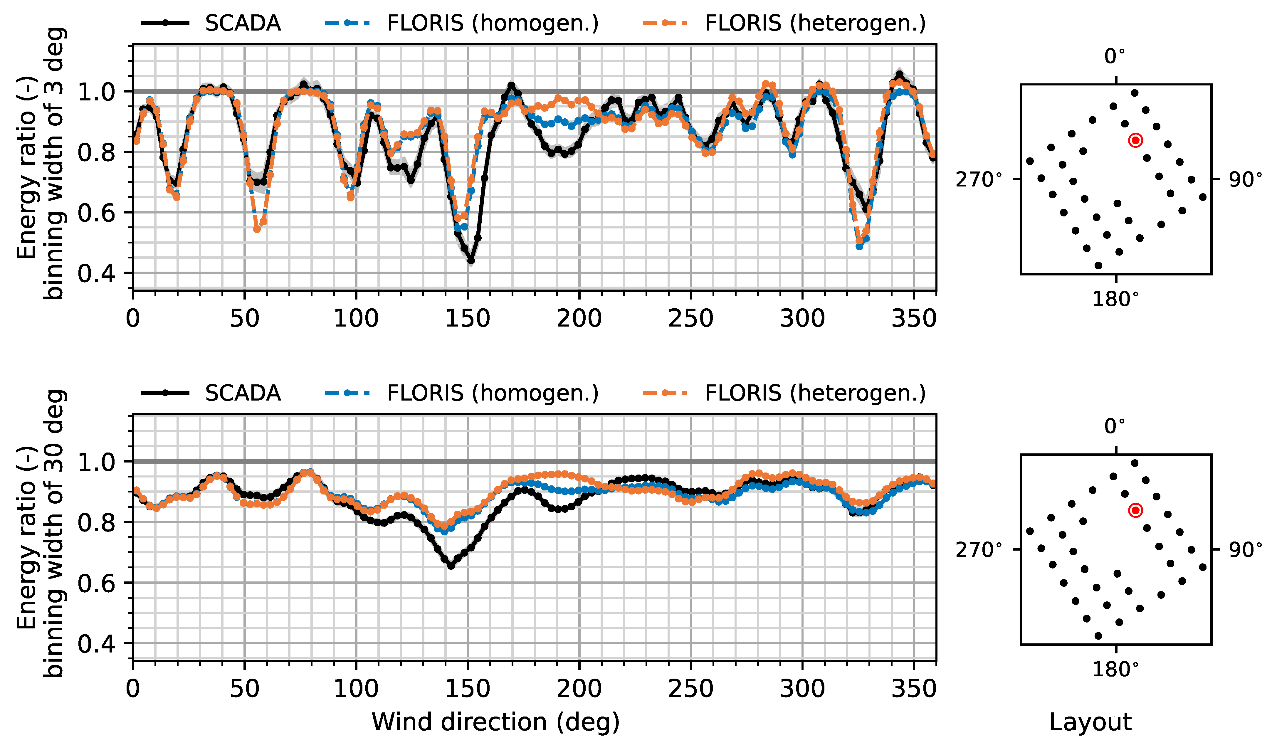
6.1. Validation with Historical Data of the Anholt Offshore Wind Farm

The energy ratio for Turbine 32 in the Anholt wind farm, positioned far south in the farm, is shown in Figure 8. The reference power productions and wind speeds are derived from the five closest upstream turbines. Figure 8 shows excellent agreement between FLORIS and the SCADA data for most wind directions between 80° and 330°, both in wake depth and in wake width. The FLORIS predictions with heterogeneous inflow are better in a few situations, near wind directions of 80° and 200°, yet are mostly equal to the predictions with homogeneous inflows. This suggests that the heterogeneous inflow does not play a dominant role in the wake losses and performance of Turbine 32, or that the current model for heterogeneity is insufficient. The predicted energy ratios significantly diverge from the historical data for wind directions less than 50° and greater than 330°. For those wind directions, the wind aligns with the direction that creates wake arrays with the highest number of turbines. One such array is highlighted in Figure 9. This figure shows how the wake losses build up as we step deeper into the wind farm. Notably, Figure 9 shows that rather than building slowly, the FLORIS-predicted energy ratios very quickly diverge, at the second or third turbine in the array.

Additionally, a curve-fitting optimization yields $I_{\infty }=0.05$ and ${\sigma }_{wd}=4.0°$. Considering the non-uniqueness issue and waterbed effect of those parameters, we can be confident in the assumed values of $I_{\infty }=0.06$ and ${\sigma }_{wd}=3.0°$.

The energy ratio for Turbine 54, positioned in the center of the farm and surrounded by turbines on all sides, is shown in Figure 10. Good agreement with historical data is observed for wind directions between 10° and 110° and between 230° and 300° for the predictions with heterogeneous inflow. The benefit of including heterogeneity in the FLORIS simulations is significant when assessing Turbine 54. Generally, the model is accurate and diverges for specific wind direction sectors, namely from 110° to 210°, and from 300° to 350°. Those regions represent situations with wind coming from the north or south, in which we expect a large number of wake interactions and wake accumulation with multiple turbines aligned, all causing wake losses on the next downstream turbine. This is very similar to the largest source of discrepancy for Turbine 32 (Figure 8).

To further assess this deep-farm effect, we consider two turbine arrays on the outer edges of the wind farm. Figure 11 and Figure 12 show that historical data from arrays of ten or more turbines, sometimes identified in the literature as “deep-array effects“, do not consistently deviate from the model-predicted energy ratios. The two curves have a slight mismatch, which is likely due to choosing a too low value for the turbulence intensity, rather than to a fundamental modeling mismatch. Considering Figure 9, it seems more likely that turbines deep in a wind farm (i.e., surrounded by many turbines) experience larger wake losses than turbines on the outer edges of the wind farm. Turbines positioned centrally in the farm have generally slower wind in their vicinity, thereby diminishing wake recovery. This model error was previously identified and addressed in the articles by Bastankhah et al. [50] and Nygaard et al. [30]. Such effects are not currently considered in the Gaussian model in FLORIS and are likely the explanation of the significant model discrepancies for wind directions from the north and south.

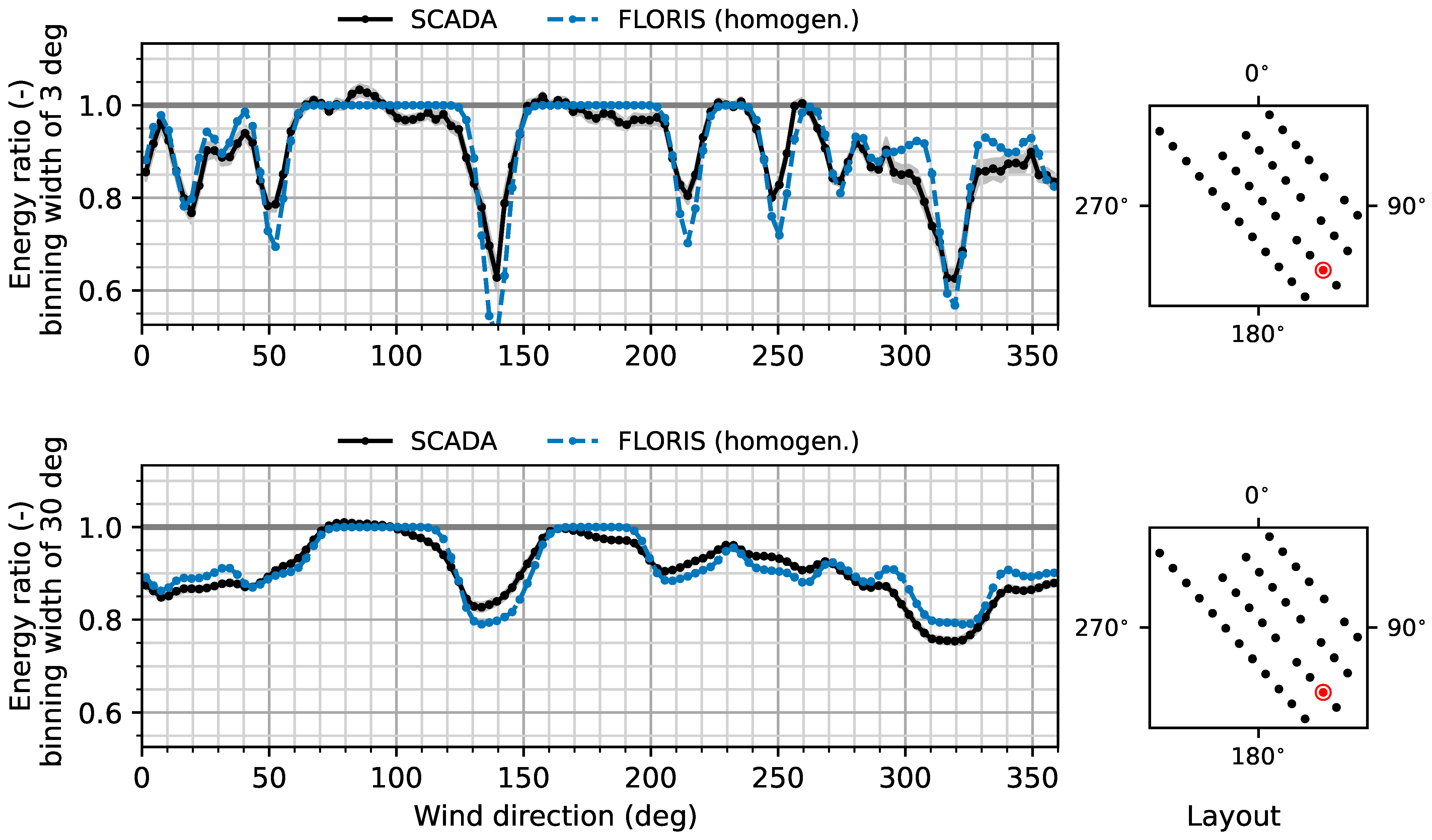
6.2. Validation with Historical Data of the Westermost Rough Offshore Wind Farm

The Westermost Rough wind farm has 35 wind turbines and is thereby the smallest wind farm discussed in this article. However, Westermost Rough is the most recently constructed farm and includes newer offshore wind turbines, each with a rated power of 6.0 MW. This section presents the energy ratios for Turbines 16 and 25. These two turbines are positioned in the central southwest and central northeast part of the farm, respectively, both adjacent to other turbines in all directions, and are thereby likely to experience significant wake effects for the entire wind rose.

Figure 13 shows the energy ratios for Turbine 16. We find excellent agreement between FLORIS and the historical data for nearly the entire wind rose, with exceptions being the sectors between 350° and 40°, and between 260° and 310°. The general trend is that wakes are underpredicted by the FLORIS model, both with and without heterogeneity in the inflow. This may have to do with the fact that the English coast is about 8 km to the southwest of the wind farm. Wind coming from this direction often has higher turbulence than winds from the sea, and are likely to induce more wake recovery, which could explain the divergence at the wind direction sector near 280°. Additionally, a second source of discrepancy may be the relatively large “opening” in the farm. For example, the distance between Turbines 27 and 16 is 29 D, which is very large for wind farm control applications, yet typically not large enough for the flow to fully recover. FLORIS has not previously been used for such large turbine spacing. Additionally, Nygaard et al. [30] confirmed that the Jensen wake model underestimates the wake depth very far downstream (see Figure 3 therein), which would agree with our observations for wind directions near 0° in Figure 13. Nygaard et al. [30] propose that such wake models are inaccurate over large distances because mixing at such distance is predominantly driven by atmospheric turbulence, and thus is not comparable to mixing over small distances, which is predominantly driven by turbine-induced turbulence. Such effects can be validated by zooming in on a single array of turbines and their wake losses, as in Figure 14. This figure and Figure 13 show that large inter-turbine spacing is not necessarily, or at least not consistently, a source of discrepancy. The FLORIS model with homogeneous inflows is very accurate for this irregularly spaced turbine array. Note that the FLORIS model with heterogeneous inflow has significant divergence, and that suggests that the heterogeneity in Westermost Rough for this wind direction sector is irregular and/or hard to predict with the current data set.

Furthermore, it is interesting to note that the effects of the neighboring Humber Gateway wind farm as described in Nygaard et al. [30] do not come forward in Figure 13, and FLORIS is accurate despite not modeling this wind farm. It is likely that the wake generated by the Humber Gateway farm presents itself in a similar manner as a freestream wind speed change upstream of the Westermost Rough wind farm. Furthermore, a curve-fitting optimization yields a minimal root mean square error with ${\sigma }_{wd}=5.5°$ and $I_{\infty }=0.03$. The estimated value for $I_{\infty }$ seems particularly low, even for offshore conditions. In conjunction with the high estimated value for ${\sigma }_{wd}$, it is likely that this is a manifestation of the waterbed effect.

Figure 15 shows the FLORIS predictions and historical data for the energy ratios of Turbine 25. The curves generally align very well for wind directions below 120° and above 220°. The wake recovery is underpredicted for 220–250°, likely due to coastal effects. Model discrepancies are significant between 100° and 200°. The largest wake deficit occurs when the wakes of Turbines 21, 22, 23, and 24 align and overlap Turbine 25. This situation is highlighted in Figure 16. This figure shows a consistently underestimated wake depth, which suggests a mismatch in the assumed ambient turbulence intensity. Additionally, the wake depth in the top plot of Figure 15 is predicted well for the wind direction of 150°, yet the wake width is underestimated, and therefore the plot with the larger bin width (bottom plot) shows a much too shallow wake in the FLORIS predictions. This is consistent with the observations of Nygaard et al. [30]. It is uncertain why the predicted wake width differs significantly with the historical data at 150° while it matches very well for other directions (e.g., at 0–100° and 250–360°). One possible explanation is the significant “gap” in the farm, yet the results for Turbine 16 suggest that the gap is not necessarily a source of error. Investigating a second turbine array with a large inter-turbine gap (Figure 17) confirms that a large inter-turbine spacing by itself is not the reason for model divergence. A secondary explanation for the model discrepancies is coastal effects and their relationship with the heterogeneity of the inflow conditions. Figure 14 and Figure 17 highlight the difficulty in accurately deriving and modeling those heterogeneous effects.

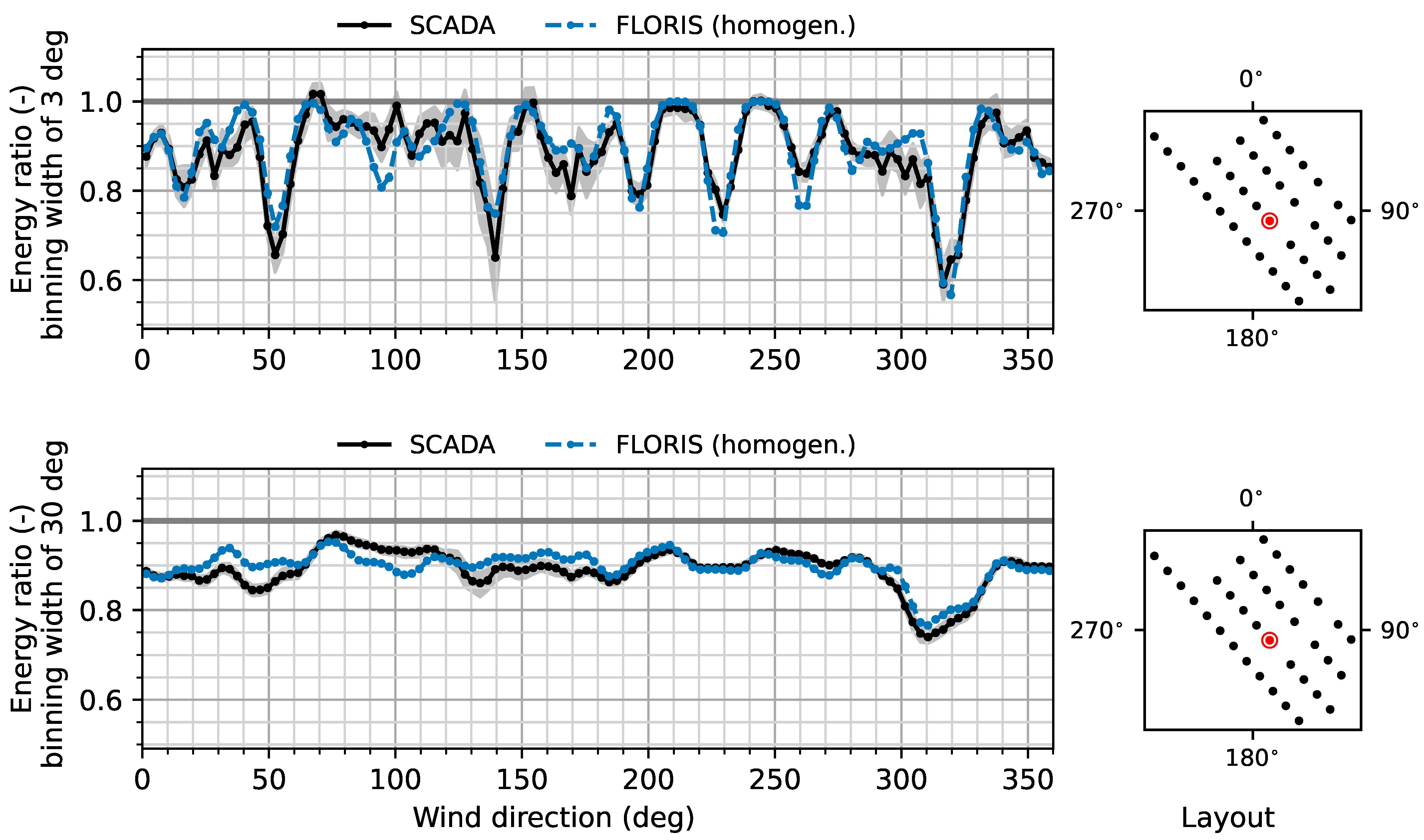
6.3. Validation with Historical Data of the OWEZ Offshore Wind Farm

The OWEZ wind farm is significantly smaller than the Anholt wind farm, with only 36 wind turbines compared with Anholt’s 111 wind turbines. Additionally, OWEZ has turbines spaced furthest apart at an average of 7.2 D, as presented in Table 1. The energy ratios of test Turbine 13 and test Turbine 16 are shown in Figure 18 and Figure 19, respectively. These two turbines are positioned in the southwest and in the center of the farm, respectively. The heterogeneous inflow curves showed larger inconsistencies due to a lack of valid data. Therefore, no FLORIS simulations with heterogeneous inflow are presented for OWEZ.

At first impression, Figure 18 shows excellent agreement between FLORIS and the SCADA data for the wake interactions. Wake losses are slightly overpredicted in certain regions, such as in the region between 100° and 160°, and slightly underpredicted for other regions, such as for wind directions between 160° and 200°, but these discrepancies are marginal. Generally, the wake deficits and wake locations are very well described. The wakes in the SCADA data are generally wider than according to FLORIS, suggesting that the assumed wind direction variability ${\sigma }_{wd}$ may be too low for the OWEZ wind farm. Indeed, a curve-fitting optimization yields optimal values of ${\sigma }_{wd}=6.0°$ and $I_{\infty }=0.04$. The value for ${\sigma }_{wd}$ is higher than anticipated. Possible explanations for this are the waterbed effect with $I_{\infty }$, direction measurement outliers, and inferior tracking of natural wind direction variations by the turbines. The last reason does not seem unreasonable, considering that this wind farm was commissioned in 2007, making it the oldest wind farm of the three investigated in this article. Furthermore, Figure 19 shows excellent agreement for the entire wind rose, with slight model discrepancies near wind directions of 50° and 100°. This may also be related to coastal effects from the Dutch shore, located to the West and Southwest of the wind farm. However, as these discrepancies are subtle and appear inconsistent for various arrays in the farm, it can not be attributed to a specific aerodynamic phenomena or model discrepancy.

7. Conclusions

This article presented a validation study of the popular Gaussian wake model implemented in NREL’s open-source FLORIS framework. This simplified wind farm model was compared to historical SCADA data of three offshore wind farms located in the North Sea in Europe. The wind farms vary in spacing from $4.9$ D to $7.2$ D and vary in number of wind turbines from 35 to 111. The historical data were preprocessed to remove the sensor-stuck type of faults, turbine curtailment, outliers on the performance curves, and data that were self-classified as bad. Moreover, using the energy ratio method, bias in the wind direction measurements of each turbine could be estimated and the turbines calibrated to true north. This method was shown to yield consistently reliable results and is able to outperform the standard method of aligning a turbine’s largest wake deficit with the direction between its closest neighboring turbine.

The model contains various input parameters, such as the wind direction variability and uncertainty, ${\sigma }_{wd}$, and the ambient turbulence intensity, $I_{\infty }$. Because of a lack of information and consensus on the definitions of these parameters, they were picked based on common values in the literature and fixed at ${\sigma }_{wd}=3.0°$ and $I_{\infty }=0.06$. In a field experiment setting, it is suggested that these two parameters are tuned to better match the model with the historical data, or possibly even estimate these parameters in real time [51]. Additionally, the default set of wake-deficit and additive-turbulence model parameters was used for the remainder of the study. Heterogeneity in the inflow wind speeds was derived from the SCADA data, and FLORIS evaluations were made with both heterogeneous and homogeneous inflows due to a lack of maturity of the heterogeneity submodel in FLORIS. The inflow heterogeneity derived from the historical data of the OWEZ wind farm showed significant inconsistencies and was not used in the remainder of the analysis.

The model predictions and the historical data were compared using the energy ratio metric. Generally, excellent agreement was found between the Gaussian wake model and historical data for most wind directions. Both the wake depth and the wake width are predicted accurately for all three wind farms. There are two areas where the model predictions diverge from the historical data. The first area where the Gaussian wake model diverges from historical data is for deep array effects, as observed in the Anholt wind farm. In the situation in which multiple wakes overlap and wind turbines are centrally positioned in the wind farm, FLORIS consistently underpredicts the wake depth. Additionally, a second discrepancy cannot be pinpointed, but is likely related to inflow heterogeneity (i.e., blockage effects, coastal effects, and effects of neighboring wind farms). Additionally, the Westermost Rough wind farm has a large “gap” in the center of the wind farm, which Nygaard et al. [30] suggested may be a reason for model divergence. Our results contradict that hypothesis and show that the Gaussian model in FLORIS is consistently accurate for such gap effects and large inter-turbine spacing.

Additionally, the issue of the “waterbed effect” was raised for ${\sigma }_{wd}$ and $I_{\infty }$, posing a non-uniqueness issue with these parameters. Different combinations of these parameters may yield nearly identical energy ratio curves, yet have fundamentally different effects when wake steering is considered. Suggestions are made to address this issue, but further pursuit is outside the scope of this work.

The results in this article demonstrate that the Gaussian wake model is an excellent choice for use in smaller offshore wind farms such as OWEZ and Westermost Rough. The model shows excellent agreement with the default sensors on the wind turbines and for turbines of different size and age. Note that the effect of wake deflection has not been explicitly tested in this study. The turbines were all operated in conventional commercial operation and thus all turbines were controlled to always be aligned with the inflow wind direction. Hence, this study has focused on validating the wake deficit and shape for the entire wind rose.

Future work should address the two aforementioned discrepancies in the Gaussian wake model. Additionally, validation studies should be performed that include common wind farm control techniques such as wake steering and axial induction control. Finally, historical data from land-based wind farms would provide very useful insights that the current model lacks for unique conditions that do not arise in offshore applications. A comparison with such historical data would further provide insight into the strengths and flaws of the current mathematical models used in wind farm control applications. Such a revised model would then make an excellent candidate for wind farm control field experiments at large offshore wind farms.

References

1. Siemens-Gamesa Renewable Energy. Wake Adapt Solution, 2019. Promotional Video; Product Advertisement. Available online: https://www.siemensgamesa.com/en-int (accessed on 4 March 2022).
2. Fleming, P.A.; Annoni, J.R.; Shah, J.J.; Wang, L.; Ananthan, S.; Zhang, Z.; Hutchings, K.; Wang, P.; Chen, W.; Chen, L. Field test of wake steering at an offshore wind farm. Wind. Energy Sci. 2017, 2, 229–239. [Google Scholar] [CrossRef] [Green Version]
3. Howland, M.F.; Lele, S.K.; Dabiri, J.O. Wind farm power optimization through wake steering. Proc. Natl. Acad. Sci. USA 2019, 116, 14495–14500. [Google Scholar] [CrossRef] [PubMed] [Green Version]
4. Fleming, P.A.; King, J.R.; Dykes, K.; Simley, E.; Roadman, J.; Scholbrock, A.K.; Murphy, P.; Lundquist, J.K.; Moriarty, P.J.; Fleming, K.; et al. Initial results from a field campaign of wake steering applied at a commercial wind farm—Part 1. Wind. Energy Sci. 2019, 4, 273–285. [Google Scholar] [CrossRef] [Green Version]
5. Fleming, P.A.; King, J.R.; Simley, E.; Roadman, J.; Scholbrock, A.; Murphy, P.; Lundquist, J.K.; Moriarty, P.J.; Fleming, K.; van Dam, J.; et al. Continued results from a field campaign of wake steering applied at a commercial wind farm—Part 2. Wind. Energy Sci. 2020, 5, 945–958. [Google Scholar] [CrossRef]
6. Doekemeijer, B.M.; Kern, S.; Kanev, S.K.; Salbert, B.; Schreiber, J.; Campagnolo, F.; Bottasso, C.L.; Maturu, S.; Schuler, S.; Wilts, F.; et al. Field experiment for open-loop yaw-based wake steering at a commercial onshore wind farm in Italy. Wind. Energy Sci. 2021, 6, 159–176. [Google Scholar] [CrossRef]
7. Fleming, P.A.; Sinner, M.; Young, T.; Lannic, M.; King, J.R.; Simley, E.; Doekemeijer, B.M. Experimental results of wake steering using fixed angles. Wind. Energy Sci. Discuss. 2021, 2021, 1–18. [Google Scholar] [CrossRef]
8. Simley, E.; Fleming, P.A.; Girard, N.; Alloin, L.; Godefroy, E.; Duc, T. Results from a Wake Steering Experiment at a Commercial Wind Plant: Investigating the Wind Speed Dependence of Wake Steering Performance. Wind. Energy Sci. Discuss. 2021, 2021, 1–39. [Google Scholar] [CrossRef]
9. Van Wingerden, J.W.; Fleming, P.A.; Göçmen, T.; Eguinoa, I.; Doekemeijer, B.M.; Dykes, K.; Lawson, M.; Simley, E.; King, J.R.; Astrain, D.; et al. Expert Elicitation on Wind Farm Control. Sci. Mak. Torque Wind. 2020, 1618, 22025. [Google Scholar] [CrossRef]
10. Fleming, P.A.; van Wingerden, J.W.; Simley, E.; Bay, C.; Doekemeijer, B.M.; Doane, H. Survey prior to kickoff meeting. IEA Task 2021, 2021, 44. [Google Scholar]
11. Boersma, S.; Doekemeijer, B.M.; Gebraad, P.M.O.; Fleming, P.A.; Annoni, J.R.; Scholbrock, A.K.; Frederik, J.A.; van Wingerden, J.W. A tutorial on control-oriented modeling and control of wind farms. In Proceedings of the American Control Conference (ACC), Seattle, WA, USA, 24–26 May 2017; pp. 1–18. [Google Scholar]
12. Crespo, A.; Hernández, J.; Frandsen, S. Survey of modelling methods for wind turbine wakes and wind farms. Wind Energy 1999, 2, 1–24. [Google Scholar] [CrossRef]
13. Rados, K.; Larsen, G.; Barthelmie, R.; Schlez, W.; Lange, B.; Schepers, G.; Hegberg, T.; Magnisson, M. Comparison of Wake Models with Data for Offshore Windfarms. Wind Eng. 2001, 25, 271–280. [Google Scholar] [CrossRef] [Green Version]
14. Machielse, L.A.H.; Schepers, J.G.; Eecen, P.J.; Korterink, H.; van de Pijl, S.P. ECN Test Farm Measurements for Validation of Wake Models; Technical Report ECN-M–07-044; TNO: Petten, The Netherlands, 2007. [Google Scholar]
15. Renkema, D.J. Validation of Wind Turbine Wake Models. Master’s Thesis, Technical University of Delft, Delft, The Netherlands, 2007. [Google Scholar]
16. Jensen, N.O. A note on Wind Generator Interaction; Technical Report RISØ-M-2411; Risø National Laboratory: Roskilde, Denmark, 1983. [Google Scholar]
17. Ainslie, J.F. Development of an eddy viscosity model for wind turbine wakes. In Proceedings of the 7th BWEA Wind Energy Conference, Oxford, UK, 27–29 March 1985. [Google Scholar]
18. Barthelmie, R.J.; Frandsen, S.T.; Nielsen, M.N.; Pryor, S.C.; Rethore, P.E.; Jørgensen, H.E. Modelling and measurements of power losses and turbulence intensity in wind turbine wakes at Middelgrunden offshore wind farm. Wind Energy 2007, 10, 517–528. [Google Scholar] [CrossRef]
19. Katic, I.; Højstrup, J.; Jensen, N.O. A simple model for cluster efficiency. In Proceedings of the European Wind Energy Conference and Exhibition (EWEC), Rome, Italy, 6–8 October 1987; Volume 1, pp. 407–410. [Google Scholar]
20. Barthelmie, R.J.; Hansen, K.; Frandsen, S.T.; Rathmann, O.; Schepers, J.G.; Schlez, W.; Phillips, J.; Rados, K.; Zervos, A.; Politis, E.S.; et al. Modelling and measuring flow and wind turbine wakes in large wind farms offshore. Wind Energy 2009, 12, 431–444. [Google Scholar] [CrossRef]
21. Barthelmie, R.J.; Pryor, S.C.; Frandsen, S.T.; Hansen, K.S.; Schepers, J.G.; Rados, K.; Schlez, W.; Neubert, A.; Jensen, L.E.; Neckelmann, S. Quantifying the Impact of Wind Turbine Wakes on Power Output at Offshore Wind Farms. J. Atmos. Ocean. Technol. 2010, 27, 1302–1317. [Google Scholar] [CrossRef]
22. Beaucage, P.; Robinson, N.; Alonge, C.; Brower, M. Overview of Six Commercial and Research Wake Models for Large Offshore Wind Farms. In Proceedings of the European Wind Energy Conference and Exhibition, Copenhagen, Denmark, 16–19 April 2012. [Google Scholar]
23. Gaumond, M.; Réthoré, P.E.; Ott, S.; Peña, A.; Bechmann, A.; Hansen, S. Evaluation of the wind direction uncertainty and its impact on wake modeling at the Horns Rev offshore wind farm. Wind Energy 2014, 17, 1169–1178. [Google Scholar] [CrossRef] [Green Version]
24. Nygaard, N.G. Wakes in very large wind farms and the effect of neighbouring wind farms. J. Physics Conf. Ser. 2014, 524, 012162. [Google Scholar] [CrossRef]
25. Nygaard, N.G. Systematic Quantification of Wake Model Uncertainty; European Wind Energy Association: Brussels, Belgium, 2015; pp. 1–10. [Google Scholar]
26. Tian, L.; Zhu, W.; Shen, W.; Zhao, N.; Shen, Z. Development and validation of a new two-dimensional wake model for wind turbine wakes. J. Wind. Eng. Ind. Aerodyn. 2015, 137, 90–99. [Google Scholar] [CrossRef] [Green Version]
27. Walker, K.; Adams, N.; Gribben, B.; Gellatly, B.; Nygaard, N.G.; Henderson, A.; Marchante Jimémez, M.; Schmidt, S.R.; Rodriguez Ruiz, J.; Paredes, D.; et al. An evaluation of the predictive accuracy of wake effects models for offshore wind farms. Wind Energy 2016, 19, 979–996. [Google Scholar] [CrossRef]
28. Archer, C.L.; Vasel-Be-Hagh, A.; Yan, C.; Wu, S.; Pan, Y.; Brodie, J.F.; Maguire, A.E. Review and evaluation of wake loss models for wind energy applications. Appl. Energy 2018, 226, 1187–1207. [Google Scholar] [CrossRef]
29. Nygaard, N.G.; Newcombe, A.C. Wake behind an offshore wind farm observed with dual-Doppler radars. J. Physics: Conf. Ser. 2018, 1037, 072008. [Google Scholar] [CrossRef]
30. Nygaard, N.G.; Steen, S.T.; Poulsen, L.; Pedersen, J.G. Modelling cluster wakes and wind farm blockage. J. Phys. Conf. Ser. 2020, 1618, 062072. [Google Scholar] [CrossRef]
31. Hamilton, N.; Bay, C.J.; Fleming, P.A.; King, J.; Martínez-Tossas, L.A. Comparison of modular analytical wake models to the Lillgrund wind plant. J. Renew. Sustain. Energy 2020, 12, 053311. [Google Scholar] [CrossRef]
32. Jiménez, A.; Crespo, A.; Migoya, E. Application of a LES technique to characterize the wake deflection of a wind turbine in yaw. Wind Energy 2010, 13, 559–572. [Google Scholar] [CrossRef]
33. Bastankhah, M.; Porté-Agel, F. Experimental and theoretical study of wind turbine wakes in yawed conditions. J. Fluid Mech. 2016, 806, 506–541. [Google Scholar] [CrossRef]
34. Martínez-Tossas, L.A.; Annoni, J.R.; Fleming, P.A.; Churchfield, M.J. The Aerodynamics of the Curled Wake: A Simplified Model in View of Flow Control. Wind. Energy Sci. 2019, 4, 127–138. [Google Scholar] [CrossRef] [Green Version]
35. King, J.; Fleming, P.A.; King, R.; Martínez-Tossas, L.A.; Bay, C.J.; Mudafort, R.; Simley, E. Control-oriented model for secondary effects of wake steering. Wind. Energy Sci. 2021, 6, 701–714. [Google Scholar] [CrossRef]
36. Ahmad, T.; Coupiac, O.; Petit, A.; Guignard, S.; Girard, N.; Kazemtabrizi, B.; Matthews, P.C. Field Implementation and Trial of Coordinated Control of WIND Farms. IEEE Trans. Sustain. Energy 2018, 9, 1169–1176. [Google Scholar] [CrossRef] [Green Version]
37. van der Hoek, D.; Kanev, S.; Allin, J.; Bieniek, D.; Mittelmeier, N. Effects of axial induction control on wind farm energy production—A field test. Renew. Energy 2019, 140, 994–1003. [Google Scholar] [CrossRef]
38. Bossanyi, E.; Ruisi, R. Axial induction controller field test at Sedini wind farm. Wind. Energy Sci. 2021, 6, 389–408. [Google Scholar] [CrossRef]
39. NREL. FLASC: A Rich Floris-Driven Suite for SCADA Analysis. Version 0.1. 2022. Available online: https://github.com/nrel/flasc (accessed on 4 March 2022).
40. Quick, J.; Annoni, J.; King, R.; Dykes, K.; Fleming, P.; Ning, A. Optimization Under Uncertainty for Wake Steering Strategies. J. Phys. Conf. Ser. 2017, 854, 012036. [Google Scholar] [CrossRef]
41. Rott, A.; Doekemeijer, B.M.; Seifert, J.; van Wingerden, J.W.; Kühn, M. Robust active wake control in consideration of wind direction variability and uncertainty. Wind Energy Sci. 2018, 3, 869–882. [Google Scholar] [CrossRef] [Green Version]
42. Simley, E.; Fleming, P.A.; King, J.R. Design and Analysis of a Wake Steering Controller with Wind Direction Variability. Wind Energy Sci. 2020, 5, 451–468. [Google Scholar] [CrossRef] [Green Version]
43. Kanev, S.; Bot, E. Dynamic robust active wake control. Wind. Energy Sci. Discuss. 2021, 2021, 1–30. [Google Scholar] [CrossRef]
44. Mittelmeier, N.; Blodau, T.; Kühn, M. Monitoring offshore wind farm power performance with SCADA data and an advanced wake model. Wind Energy Sci. 2017, 2, 175–187. [Google Scholar] [CrossRef]
45. Gebraad, P.M.O.; Teeuwisse, F.W.; van Wingerden, J.W.; Fleming, P.A.; Ruben, S.D.; Marden, J.R.; Pao, L.Y. Wind plant power optimization through yaw control using a parametric model for wake effects—A CFD simulation study. Wind Energy 2016, 19, 95–114. [Google Scholar] [CrossRef]
46. IEA-Wind. IEA Wind Task 44. 2021. Available online: https://iea-wind.org/task44/ (accessed on 4 March 2022).
47. Efron, B.; Tibshirani, R.J. An Introduction to the Bootstrap; Chapman & Hall: London, UK, 1993. [Google Scholar]
48. NREL. FLORIS. Version 2.4. 2021. Available online: https://github.com/nrel/floris (accessed on 4 March 2022).
49. Farrell, A.; King, J.; Draxl, C.; Mudafort, R.; Hamilton, N.; Bay, C.J.; Fleming, P.; Simley, E. Design and analysis of a wake model for spatially heterogeneous flow. Wind Energy Sci. 2021, 6, 737–758. [Google Scholar] [CrossRef]
50. Bastankhah, M.; Welch, B.L.; Martínez-Tossas, L.A.; King, J.; Fleming, P.A. Analytical solution for the cumulative wake of wind turbines in wind farms. J. Fluid Mech. 2021, 911, A53. [Google Scholar] [CrossRef]
51. Doekemeijer, B.M.; van der Hoek, D.C.; van Wingerden, J.W. Closed-loop model-based wind farm control using FLORIS under time-varying inflow conditions. Renew. Energy 2020, 156, 719–730. [Google Scholar] [CrossRef]
52. Bastankhah, M.; Porté-Agel, F. A new analytical model for wind-turbine wakes. Renew. Energy 2014, 70, 116–123. [Google Scholar] [CrossRef]
53. Crespo, A.; Hernández, J. Turbulence characteristics in wind-turbine wakes. J. Wind. Eng. Ind. Aerodyn. 1996, 61, 71–85. [Google Scholar] [CrossRef]
Figure 1. Layouts of the three wind farms: Anholt, Egmond Aan Zee (OWEZ), and Westermost Rough.
Energies 15 01964 g001
Figure 2. Performance curve for an imaginary wind turbine with artificially generated data, demonstrating the filtering process. The green dots indicate outliers and a curtailment region between normalized wind speeds 0.4 and 0.75, where the power is curtailed to 70% of the wind turbine’s rated value. Additionally, data points above rated wind speed but far below rated power are removed. Data marked in orange are all data with a power more than 5 kW above the rated value and are also removed.
Energies 15 01964 g002
Figure 3. Example of the Northing calibration by optimizing the Pearson correlation coefficient between FLORIS predictions and the SCADA data for various bias correction values. The example shows the energy ratio curves for the Anholt wind farm, test Turbine 32. The reference turbines are the upstream turbines within a 5 km radius, and the reference wind direction measurement (which is calibrated) is the average of the wind direction measurements reported by Turbines 30 and 31. The layout schematic on the right shows the location of Turbine 32 in the wind farm.
Energies 15 01964 g003
Figure 4. The effect of different bin widths (3° vs. 30°) on the energy ratio curves for test Turbine 32 of the Anholt wind farm. The reference turbines are all upstream turbines within a 5 km radius, and the reference wind direction is the measured wind direction at Turbines 30 and 31. The energy ratios are calculated every 3°. Wider bins provide more overlap and smoother wake profiles (e.g., near 145°). Yet wider bins also blend out wake profiles otherwise observed in the data (e.g., between 200° and 300°). The layout schematic on the right shows the location of Turbine 32 in the wind farm.
Energies 15 01964 g004
Figure 5. The effect of different atmospheric turbulence intensities and inflow wind direction standard deviations on the energy ratio of test Turbine 32 in the Anholt wind farm. The choice of atmospheric turbulence intensity and inflow wind direction variability in the FLORIS model exclusively change the energy ratios of the model-generated data. The layout schematic on the right shows the location of Turbine 32 in the wind farm.
Energies 15 01964 g005
Figure 6. The energy ratios for all upstream wind turbines at the Anholt wind farm normalized to the average of all turbines for a wind sector of 262.5 ° to 277.5 ° , equal to wind coming from the west. For this wind direction, turbines very south in the farm (e.g., T0, T1) generate 15 % less energy than the average of all upstream turbines, whereas turbines far north in the farm (e.g., T63, T64) generate 10 % more. The shaded region represents 90% confidence intervals.
Energies 15 01964 g006
Figure 7. The energy ratios for all upstream wind turbines at the Westermost Rough wind farm normalized to the average of all turbines for a wind sector of 262.5 ° to 277.5 ° , equal to wind coming from the west. For this wind direction, turbines central in the farm (e.g., T3, T4) generate up to 5 % less energy than the average of all upstream turbines, whereas turbines far north in the farm (e.g., T27, T34) generate 5 % 8 % more. The shaded region represents 90% confidence intervals.
Energies 15 01964 g007
Figure 8. Energy ratio curves for Turbine 32 in the Anholt wind farm, in which the reference turbines are the five closest upstream turbines, and the reference wind direction is the average of the wind direction measurements of neighboring Turbines 30, 31, 33, and 42. The shaded regions represent 90 % confidence interval bounds obtained through bootstrapping. The layout schematic on the right shows the location of Turbine 32 in the wind farm.
Energies 15 01964 g008
Figure 9. Energy ratios of Turbines 104, 103, 57, 56, 55, 54, 39, 38, 37, 36, 35, 34, 33, and 32 for a narrow wind direction sector of 348.3 ° to 3.3 ° . Turbine 104 acts as the reference turbine, and the reference wind direction is the average of the wind direction measurements of the array of turbines. The shaded regions represent 90 % confidence interval bounds obtained through bootstrapping. The layout schematic on the right shows the location of Turbines 104, 103, 57, 56, 55, 54, 39, 38, 37, 36, 35, 34, 33, and 32 in the wind farm.
Energies 15 01964 g009
Figure 10. Energy ratio curves for Turbine 54 in the Anholt wind farm, in which the reference turbines are the five closest upstream turbines, and the reference wind direction is the average of the wind direction measurements of Turbines 40, 53, 56, and 100. The shaded regions represent 90 % confidence intervals obtained through bootstrapping. The layout schematic on the right shows the location of Turbine 54 in the wind farm.
Energies 15 01964 g010
Figure 11. Energy ratios of Turbines 0 through 10 for the Anholt wind farm for a narrow wind direction sector of 172.1 ° to 187.1 ° . Turbine 0 acts as the reference turbine, and the reference wind direction is the average of the wind direction measurements of the array of turbines. The shaded regions represent 90 % confidence interval bounds obtained through bootstrapping. The layout schematic on the right shows the location of Turbines 0 through 10 in the wind farm.
Energies 15 01964 g011
Figure 12. Energy ratios of Turbines 110 through 98 for the Anholt wind farm for a narrow wind direction sector of 330.3 ° to 345.3 ° . Turbine 110 acts as the reference turbine, and the reference wind direction is the average of the wind direction measurements of the array of turbines. The shaded regions represent 90 % confidence interval bounds obtained through bootstrapping. The layout schematic on the right shows the location of Turbines 110 through 98 in the wind farm.
Energies 15 01964 g012
Figure 13. Energy ratio curves for Turbine 16 in the Westermost Rough wind farm, where the reference turbines are all upstream turbines within a 5 km radius, and the reference wind direction is the average of the nacelle headings of Turbines 9, 8, 15, and 25. The shaded regions represent 90 % confidence intervals obtained through bootstrapping. The layout schematic on the right shows the location of Turbine 16 in the wind farm.
Energies 15 01964 g013
Figure 14. Energy ratios of Turbines 0, 8, 16, 25, and 33 for the Westermost Rough wind farm for a narrow wind direction sector of 189.5 ° to 204.5 ° . Turbine 0 acts as the reference turbine, and the reference wind direction is the average of the wind direction measurements of the array of turbines. The shaded regions represent 90 % confidence interval bounds obtained through bootstrapping. The layout schematic on the right shows the location of Turbines 0, 8, 16, 25, and 33 in the wind farm.
Energies 15 01964 g014
Figure 15. Energy ratio curves for Turbine 25 in the Westermost Rough wind farm, where the reference turbines are all upstream turbines within a 5 km radius, and the reference wind direction is the average of the nacelle headings of Turbines 24, 27, 32, and 33. The shaded regions represent 90 % confidence intervals obtained through bootstrapping. The layout schematic on the right shows the location of Turbine 25 in the wind farm.
Energies 15 01964 g015
Figure 16. Energy ratios of Turbines 21 through 27 for the Westermost Rough wind farm for a narrow wind direction sector of 139.1 ° to 154.1 ° . Turbine 21 acts as the reference turbine, and the reference wind direction is the average of the wind direction measurements of the array of turbines. The shaded regions represent 90 % confidence interval bounds obtained through bootstrapping. The layout schematic on the right shows the location of Turbines 21 through 27 in the wind farm.
Energies 15 01964 g016
Figure 17. Energy ratios of Turbines 4, 10, 16, and 21 for the Westermost Rough wind farm for a narrow wind direction sector of 269.6 ° to 284.6 ° . Turbine 4 acts as the reference turbine, and the reference wind direction is the average of the wind direction measurements of the array of turbines. The shaded regions represent 90 % confidence interval bounds obtained through bootstrapping. The layout schematic on the right shows the location of Turbines 4, 10, 16, and 21 in the wind farm.
Energies 15 01964 g017
Figure 18. Energy ratio curves for Turbine 13 in the OWEZ wind farm, where the reference turbines are all upstream turbines within a 5 km radius, and the reference wind direction is the average of the nacelle headings of Turbines 0, 1, 15, and 22. The shaded regions represent 90 % confidence intervals obtained through bootstrapping. The layout schematic on the right shows the location of Turbine 13 in the wind farm.
Energies 15 01964 g018
Figure 19. Energy ratio curves for Turbine 16 in the OWEZ wind farm, where the reference turbines are all upstream turbines within a 5 km radius, and the reference wind direction is the average of the nacelle headings of turbines 3, 15, 17, and 24. The shaded regions represent 90 % confidence intervals obtained through bootstrapping. The layout schematic on the right shows the location of Turbine 16 in the wind farm.
Energies 15 01964 g019