Thermal and Economic Analysis of Heat Exchangers as Part of a Geothermal District Heating Scheme in the Cheshire Basin, UK

Abstract

Heat exchangers are vital to any geothermal system looking to use direct heat supplied via a district heat network. Attention on geothermal schemes in the UK has been growing, with minimal attention on the performance of heat exchangers. In this study, different types of heat exchangers are analysed for the Cheshire Basin as a case study, specifically the Crewe area, to establish their effectiveness and optimal heat transfer area. The results indicate that counter-current flow heat exchangers have a higher effectiveness than co-current heat exchangers. Optimisation of the heat exchange area can produce total savings of £43.06 million and £71.5 million, over a 25-year lifetime, in comparison with a fossil-fuelled district heat network using geothermal fluid input temperatures of 67 °C and 86 °C, respectively.

1. Introduction

For deep geothermal schemes that target conventional resources in the UK relatively little work has been undertaken analysing the effectiveness of heat exchangers for district heating schemes. Heat exchangers are important to any geothermal scheme as they ensure that the extracted heat is useable, supplying the demand directly. Low-enthalpy or low-temperature geothermal schemes usually exploit resources under 100 °C, and heat is transferred from a doublet (two-well) system through a heat exchanger which then feeds a district heat network (DHN) (Figure 1). A heat exchanger operates by transferring heat between two fluids over a given surface area, preventing corrosion and scaling caused by the geothermal fluid in the DHN [1]. Not all the heat can be transferred and, as such, the input temperature into the DHN must be evaluated. It is also important to calculate the outlet temperature of the geothermal fluid to assess further use in a cascade scheme or for geothermal modelling of the subsurface during re-injection.

The Cheshire Basin, located in the north west of England (Figure 2), is the target of this research due to the significant amount of untapped heat in place within the basin (~75 EJ), with the highest concentrations of the resource located in the subsurface below Crewe [2,3]. Furthermore, favourable temperatures and a thick succession of Permo-Triassic sandstones provide high-quality permeable aquifers [4,5,6,7]. For a heat network to be efficient there must be demand in proximity to the wellhead to minimise heat losses. In Crewe town centre, recent plans are in place to develop a DHN with demand of the initial phase to be estimated in the region of 1.6 MW [8].

Heat exchangers have been used and modelled for geothermal systems internationally. In geothermal-fed district heat networks, counter-flow plate heat exchangers are most commonly used as they have been proven to be the most effective and can offer the highest economic benefits in comparison with others (e.g., such as shell and tube) [9,10]. Counter-current flow heat exchangers transfer heat between two fluids passing in opposite directions, whilst co-current flow heat exchangers pass heat between two fluids travelling in the same direction (Figure 3). An initial comparison between counter- and co-current flow heat exchangers was undertaken to highlight the significant difference in output temperature and effectiveness. Further modelling was then undertaken to identify optimal heat exchanger surface area under varying scenarios.

Further studies on heat exchangers in geothermal systems have investigated direct heat exchange in a downhole heat exchanger geothermal system [11]. This is similar to the use of borehole heat exchangers, where fluid is not extracted from a geothermal reservoir and heat transfer occurs directly at depth via conduction through the pipe and grout (e.g., [12,13]). Earth-to-air heat exchangers have also been used in ventilation systems in temperate climate locations, highlighting that the geometry of such systems is important (e.g., [14]). In this study, we focus on heat extraction from a conventional resource using a doublet system; therefore, our work focuses on counter- and co-current flow heat exchangers.

Optimisation is useful to minimise capital investment and, thus, maximise the net profit for a heat-exchanger-fed deep geothermal scheme. The primary role of any heat exchanger used in a district heat network is to transfer heat between two fluids. As such, a larger heat exchange area is necessary to maximise heat transfer between each fluid. The optimum heat exchanger area can, therefore, be determined as the area that produces the maximum net profit, whilst allowing sufficient energy to be transferred between fluids. Previous studies have focused on the optimisation by minimising cost, whilst maximising effectiveness and heat transfer rate (e.g., [15,16]). Typically, optimisation studies of plate heat exchangers are conducted using the Genetic Algorithm (e.g., [17]) and through mathematical optimisation (e.g., [18]). In this study, we wish to determine the optimal heat transfer area and maximum net profit of a district heat exchanger of a geothermal-fed DHN; therefore, the latter mathematical optimisation is used.

After fluids pass through a heat exchanger it is important to investigate the useable energy. This can help determine whether a deep geothermal scheme can match the surface demand, including operation at both high and low demand periods. It is also useful to understand whether the savings in using a potentially cheaper source (geothermal) in comparison with typical fossil fuel boiler schemes are worthwhile. At present, financial and geological risk remains high within the Cheshire Basin and much of the UK. Although some attempts were made to reduce the geological risk, through the complex modelling of new extraction techniques such as deep borehole heat exchangers ([12,19,20]), minimal studies have observed the financial connotations. Those which have, focus on single well systems, suggesting that any profit is minimal ([21]).

In this study, the variations in production temperature and flow rate from a deep geothermal scheme are accounted for, to some extent, by modelling a range of parametric inputs to the heat exchanger. Furthermore, regression models produced can assist in predicting financial savings of a heat exchanger for different input parameters. The results can, therefore, be used for different geothermal-fed heat networks across the UK and Europe where the geology and heat network capacity are similar.

2. Method

2.1. Thermal Analysis of the Heat Exchanger

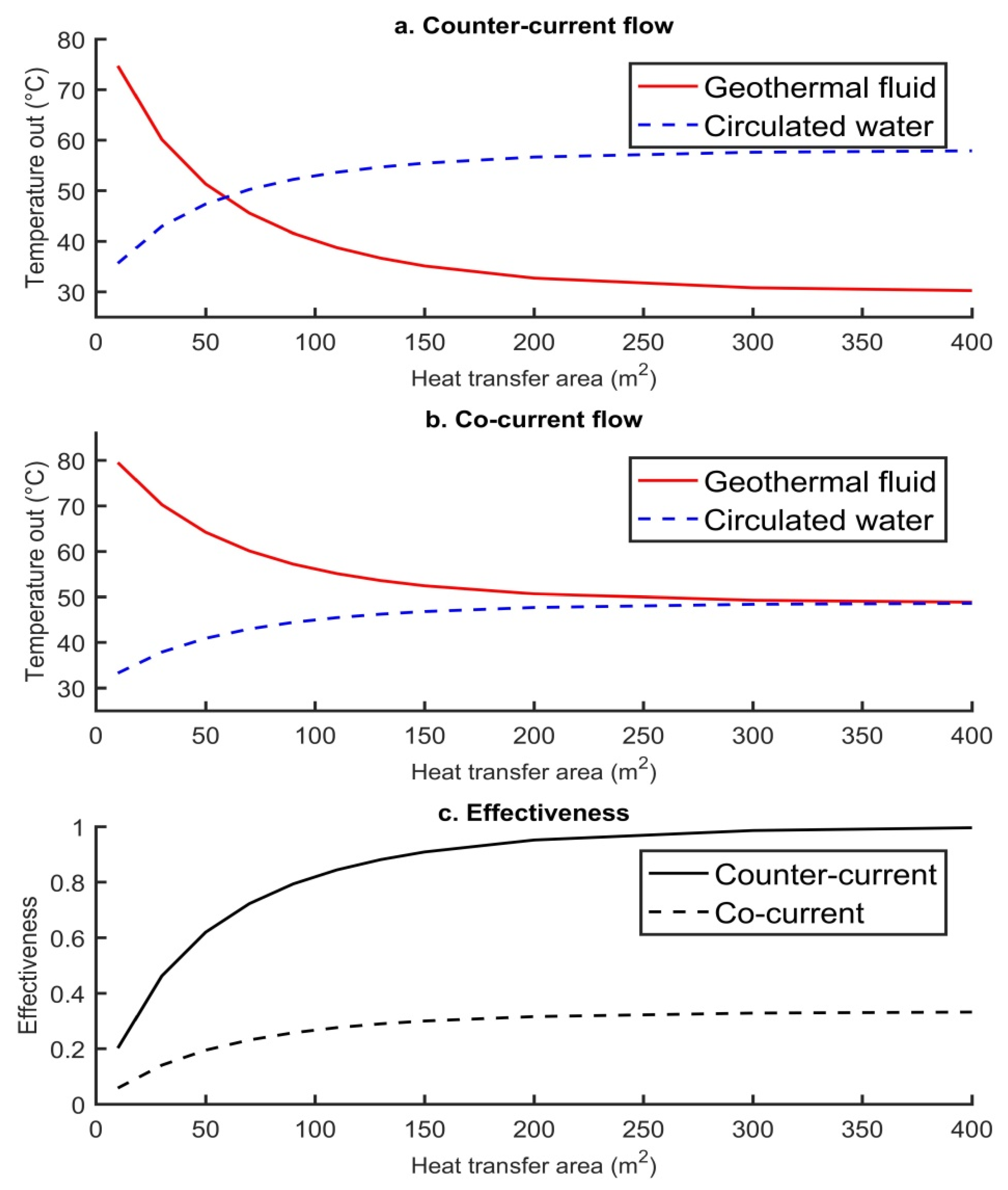
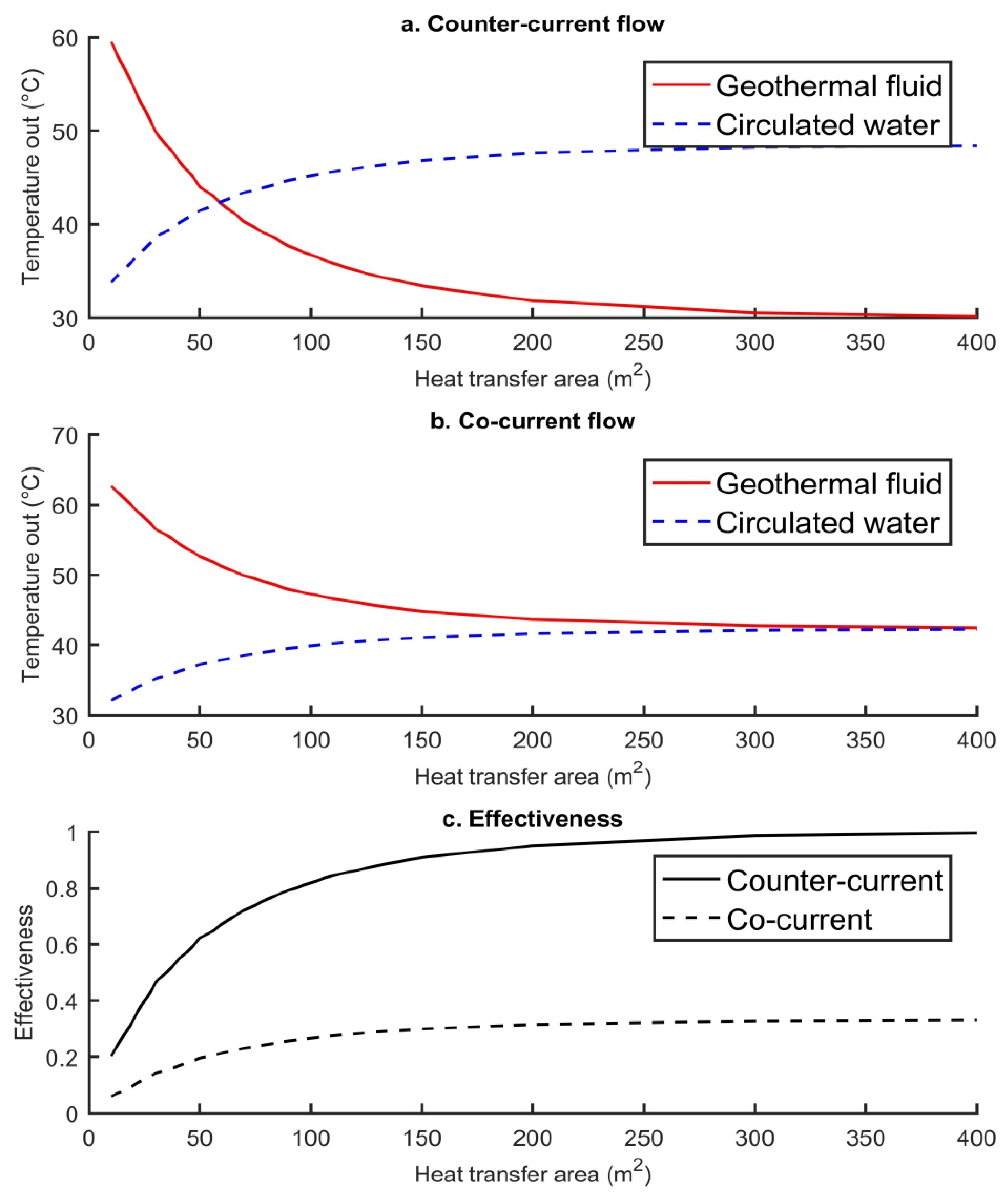
2.1.1. Counter-Current Flow Heat Exchangers

Counter-current flow heat exchangers transfer heat between two fluids travelling in opposite directions, with one fluid being the hot geothermal fluid ($T_h$) and the other a clean circulating fluid ($T_c$) (Figure 3). The output temperature of the geothermal fluid was calculated from the input temperatures into the heat exchanger ([18]):

$$T_{hout}=T_{hin}-\left(T_{hin}-T_{cin}\right) – \frac{\left(1-e^D\right)}{\left((C_h/C_c)-e^D\right)}$$

(1)

where $T$ is the temperature, $C$ is the thermal capacity, and $D$ is calculated as $D=U.A \left(\frac{1}{C_h}-\frac{1}{C_c}\right)$. The thermal capacity was calculated as $C=m.C_p$, where $m$ is the mass flow rate and $C_p$ is the specific heat capacity. The subscripts $in$ and $out$ represent the inlet or outlet into the heat exchanger, whilst subscripts $h$ and $c$ relate to the hot (geothermal) fluid and cold (clean circulating) fluid used in the district heat network. $U$ is the heat transfer coefficient and $A$ is the heat transfer area. The model also assumes that the mass flow rate for the circulatory fluid is higher than that of the geothermal fluid.

The temperature of the circulatory cold fluid was calculated by assuming that the heat transfer rate of the geothermal fluid was known ([18]):

$$C_h.\left(T_{hin}-T_{hout}\right)=C_c.\left(T_{cin}-T_{cout}\right)$$

(2)

The effectiveness (ε) was calculated as $\epsilon =\frac{\left(1-e^D\right)}{\left((C_h/C_c)-e^D\right)}$ and expressed as a value between zero and one, where zero is ineffective and one is 100% effective.

2.1.2. Co-Current Flow Heat Exchangers

Co-current flow heat exchangers involve the transfer of heat between two fluids travelling in the same direction (Figure 3) and were modelled as ([22]):

$$T_{hout}=T_{cin}+\frac{\left(T_{hin}-T_{cin}\right)}{{\left(1+(C_c/C_h)\right)}^{\left(1-e^{-\frac{U.A}{C_c}}\right)}}$$

(3)

where the effectiveness was calculated from:

$$\epsilon =(C_h/C_c).\left(1-\frac{1}{{\left(1+(C_c/C_h)\right)}^{\left(1-e^{-\frac{U.A}{C_c}}\right)}}\right)$$

(4)

Typically, counter-current flow heat exchangers are used for heat networks due to their higher efficiencies ([9,10]); however, co-current flow heat exchangers were also modelled for comparison.

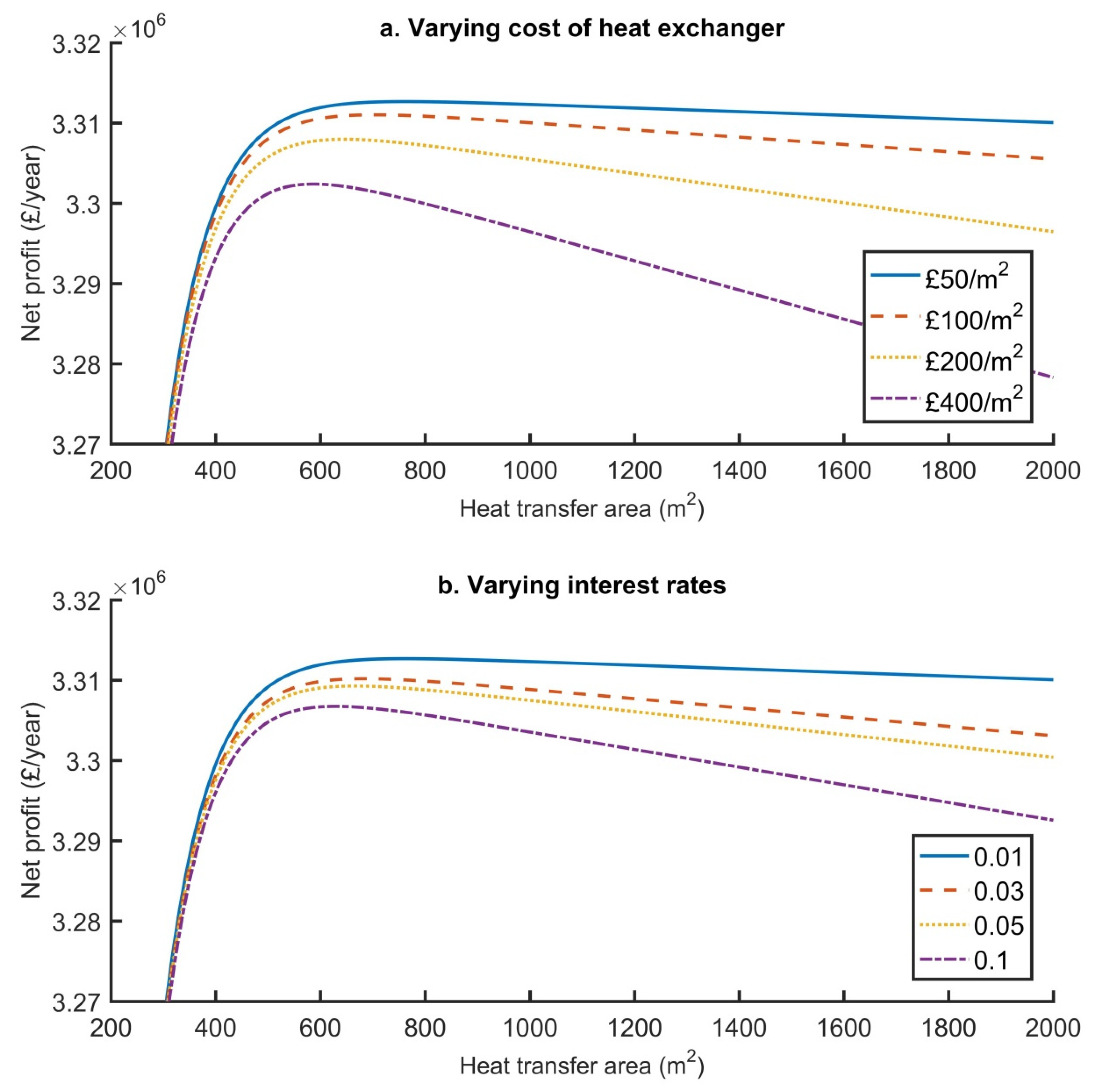
2.2. Economic Modelling

The heat exchanger is usually the most significant cost in a district heat network scheme (assuming the geothermal well has already been drilled). A cost comparison was made between installing a heat exchanger for a geothermal-fed heat network and a conventional fossil-fuelled boiler fed heat network. The total savings of using the former was calculated as follows ([18]):

The annual investment cost of a heat exchanger (C_a) was calculated as:

$$C_a=I_c.A.CRF$$

(5)

where the capital recovery factor of investment (CRF) was:

$$CRF=\frac{{\left(1+i\right)}^n.i}{{\left(1+i\right)}^n-1}$$

(6)

I_c is the cost of a heat exchanger per unit area, i is the interest rate, and n is the lifetime of the heat exchanger. The net profit (NK) supplying a district heating scheme with geothermal fluid, rather than utilising a conventional fossil-fuelled boiler, was calculated from:

$$NK=ASM-C_a$$

(7)

The annual saved money (ASM) was calculated for a conventional fossil fuel district heating system as:

$$ASM=Q.H.\frac{3600}{H_u.\eta }. F$$

(8)

where Q is the heat rate, H is the hours of plant operation, H_u is the lower heating value of fuel, η is the efficiency of the boiler, and F is the cost of fuel.

The equations were solved using MATLAB (Algorithm 1) and the optimum surface area for heat exchange was defined based on the maximum net profit (Equation (7)). Equations (1) and (2) were solved for a range of surface areas, which was incrementally increased. The heat rate (Q) was then determined for each output and Equations (5)–(8) were solved, highlighting the solution where the heat exchanger produced the highest net profit and the given surface area. A range of solutions were then tested to evaluate the impacts of varying different parameters such as interest rate, inlet temperature, and heat exchanger cost on the optimal surface area.

Algorithm 1:Determining the optimal surface area.

Input: Parameters listed in Table 1. Output: Optimal surface area and net profit   1: For A = 1:2000; % incremental increase in surface area (m2) 2:    Solve for temperature of the geothermal fluid out (Equation (1)) 3:    Solve for temperature of the clean fluid out the heat exchanger (Equation (2)) 4:    Solve for the net profit (Equation (7)) 5: end 6: Identify the largest net profit (NKmax) and respective surface area (A)

2.3. Parameterisation

A range of geothermal fluid input temperatures were modelled; these were representative of the published temperatures for the Cheshire Basin (Crewe area). Current published estimates of the temperature of the base Permian rocks in the Crewe area range between 67 °C and 86 °C ([4,23,24,25]) The lower end estimate is similar to that of using the thermal gradient from un-corrected bottom-hole temperatures, whilst the higher limit is that from using the newly corrected thermal gradient ([7]). As such, the two end-member scenarios for published temperatures were used to compare different heat exchanger configurations, in order to find the most efficient surface area of the heat exchanger and determine the maximum net profit. If the production temperature was in excess of 100 °C further modelling of Organic Rankine Cycles should be considered ([26]).

The initial analysis focused on which heat exchanger would be most effective; as such, the minimum and maximum temperature range from the literature highlighted above was used with fixed parameters, only altering the heat transfer area (parameters listed in Table 1). The inlet temperature of the circulating fluid was fixed at 30 °C as this is considered the typical rejection temperature for the UK ([4]). The initial circulation flow rate in the heat exchanger was set at 80 kg/s, and the input geothermal fluid flow rate was 40 kg/s. The high geothermal fluid flow rate of 40 kg/s was chosen to test the potential for higher capacity production. The heat transfer coefficient was set at 4000 W/m² °C. This is within the typical range of heat transfer coefficients in the literature for geothermal district heating systems, which is between 2900 and 5100 W/m² °C (e.g., [18,27]); however, it is a slightly reduced value as it is assumed that some fouling (scaling) will occur in the heat exchanger, thus reducing the performance ([28]). The heat transfer area was altered to establish the optimal configurations for both the co-current and counter-current flow heat exchangers.

The economic performance of the geothermal-fed district heat network with heat exchanger installation can be determined in comparison with its fossil-fuelled counterpart. Fossil-fuelled systems typically use a boiler, and in this study its efficiency was set at 0.85 ([29,30]). It was assumed the fuel source was heating oil (similar to diesel), which is typically used in small-scale UK domestic and commercial applications. The lower heating value was set at 43,000 kJ/kg ([31]) and the cost was 0.49 £/L (values listed in Table 1). Heat exchanger prices were modelled at current market rates, whilst interest rates were modelled at the current and historical Bank of England interest rates ([32]). Both parameters were increased to show the reduction in annual savings.

Table 1. Table of properties and nomenclature used in the simulations.

Parameter	Value
Flow rate of geothermal fluid (mh)	80 kg/s
Flow rate of circulating fluid (mc)	40 kg/s
Inlet temperature of geothermal fluid (Thin)	67 °C (min) and 86 °C (max) [4,23,24]
Inlet temperature of circulating fluid (Tcin)	30 °C [27]
Return temperature of circulating fluid (Tcout)	48.5 °C (min) and 58 °C (max)
Specific heat capacity of water (Cp)	4200 J/kg K
Heat transfer coefficient (U)	4000 W/m2 °C [18,27]
Boiler efficiency (η)	0.85 [29,30]
Cost of heat exchanger per unit area (Ic)	50 £/m2
Lower heating value of fuel (Hu)	43,000 kJ/kg [31]
Fuel cost (F)	0.49£ per litre
Interest rate (i)	0.01 [32]
Lifetime (n)	25 years

Parameters explained in Section 3.1 and Section 3.2.

Table 1. Table of properties and nomenclature used in the simulations.

Parameter	Value
Flow rate of geothermal fluid (mh)	80 kg/s
Flow rate of circulating fluid (mc)	40 kg/s
Inlet temperature of geothermal fluid (Thin)	67 °C (min) and 86 °C (max) [4,23,24]
Inlet temperature of circulating fluid (Tcin)	30 °C [27]
Return temperature of circulating fluid (Tcout)	48.5 °C (min) and 58 °C (max)
Specific heat capacity of water (Cp)	4200 J/kg K
Heat transfer coefficient (U)	4000 W/m2 °C [18,27]
Boiler efficiency (η)	0.85 [29,30]
Cost of heat exchanger per unit area (Ic)	50 £/m2
Lower heating value of fuel (Hu)	43,000 kJ/kg [31]
Fuel cost (F)	0.49£ per litre
Interest rate (i)	0.01 [32]
Lifetime (n)	25 years

Parameters explained in Section 3.1 and Section 3.2.

3. Results

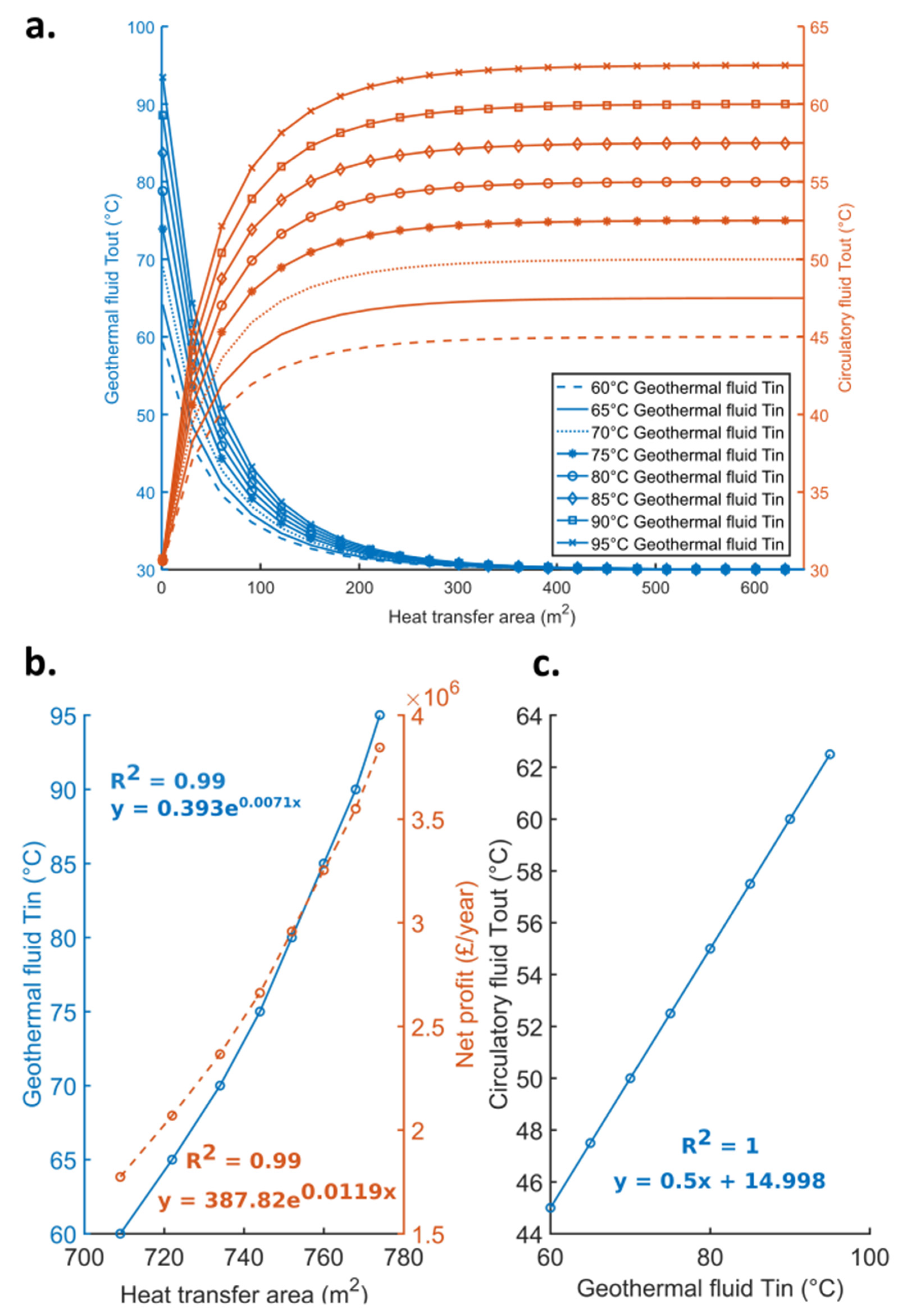
3.1. High Input Temperature of Geothermal Fluid

When analysing the higher geothermal fluid input temperature, counter-flow heat exchangers showed an exponential decrease in geothermal fluid output temperature with increasing transfer area, until it reached the circulating fluid input temperature of 30 °C (Figure 4a). The circulating fluid increased in temperature and became asymptotic to ~58 °C, which is the maximum output temperature of the clean circulatory fluid (Figure 4a). This shows that the counter-current flow exchanger is working efficiently, with most of the heat transferring to the circulatory fluid with larger surface areas. The outlet temperature for co-current flow heat exchangers, for both the geothermal fluid and circulated water, were asymptotic to ~49 °C (9 °C less than the counter-current flow heat exchanger) as the surface area increased (Figure 4b). The effectiveness of the co-current flow heat exchanger was poor in comparison and was always less than 0.34 (Figure 4c). This shows not all the energy was transferred from the geothermal fluid to the circulatory fluid. From the modelled results, it is clear that counter-current flow heat exchangers are more suited for a district heating scheme in this case, which is consistent with findings in the literature ([9,10]).

3.2. Low Input Temperature of Geothermal Fluid

For lower input temperatures (67 °C), the heat exchanger efficiency was identical to that of the higher input temperature models. However, the maximum output temperatures of the circulating fluid were far less at 42.3 °C and 48.4 °C for both co-current and counter-current flow, respectively (Figure 5). This is to be expected as the temperature of the geothermal fluid is closer to the input temperature of the circulating fluid.

3.3. Economic Analysis of Varying Heat Transfer Area for Counter-Current Flow Heat Exchangers

The cost analysis was based on that of a counter-current flow heat exchanger due to the higher efficiency identified in Section 3.1 and Section 3.2.

3.3.1. Low Temperature Geothermal Inlet Fluid

The maximum net profit increased as a consequence of the reduction in cost per m² of the heat exchanger, with a similar trend found with higher interest rates. For the minimum geothermal fluid input temperature value (67 °C), the optimal surface area of the heat exchanger was found to be 727 m² for a scheme with an interest rate of 0.01 and a low-cost value of the heat exchanger of £50 per m² (Figure 6a and Figure 7a). The optimal surface area was determined as the point that net profit would be highest (Figure 6a) and was £2.1858 million per year. For the higher cost heat exchanger of £400 per m², the optimal surface area reduced to 553 m² and net profit reduced to £2.1784 million per year (

Table 2. Optimal area compared to increasing heat exchanger cost and interest rates for an input temperature of 67 °C (of the geothermal fluid).

Heat Exchanger (£/m2)	Optimum Heat Transfer Area (m2)
50	727
100	669
200	611
400	553
Interest Rate (i)	Optimum Heat Transfer Area (m2)
0.01	727
0.03	649
0.05	631
0.1	594

, Figure 7a). Similarly, higher interest rates (0.1) resulted in an optimal surface area of 594 m² and a net profit of £2.1825 million per year (Table 2, Figure 7b).

3.3.2. High Temperature Geothermal Inlet Fluid

A higher input temperature (86 °C) for the geothermal fluid into the heat exchanger results in far higher net profits per year. An interest rate of 0.01 and cost of £50 m² gives a net profit of £3.3127 million per year and an optimal surface area of 762 m² (Figure 6b). Similar to the trend of the lower input geothermal fluid temperature’s results, the optimal surface area and net profit reduced with increasing interest rates and cost per m² of the heat exchanger. The highest heat exchanger cost (£400/m²) resulted in a net profit of £3.3024 million per year and an optimal area of 587 m² (

Table 3. Optimal area compared with increasing heat exchanger cost and interest rates for an input temperature of 86 °C (of the geothermal fluid).

Heat Exchanger Cost per m2 (£/m2)	Optimum Heat Transfer Area (m2)
50	762
100	704
200	645
400	587
Interest Rate (i)	Optimum Heat Transfer Area (m2)
0.01	762
0.03	684
0.05	666
0.1	629

, Figure 8a), whilst an interest rate of 0.1 gives a net profit of £3.3067 million per year and an optimal surface area of 629 m² (Table 3, Figure 8b).

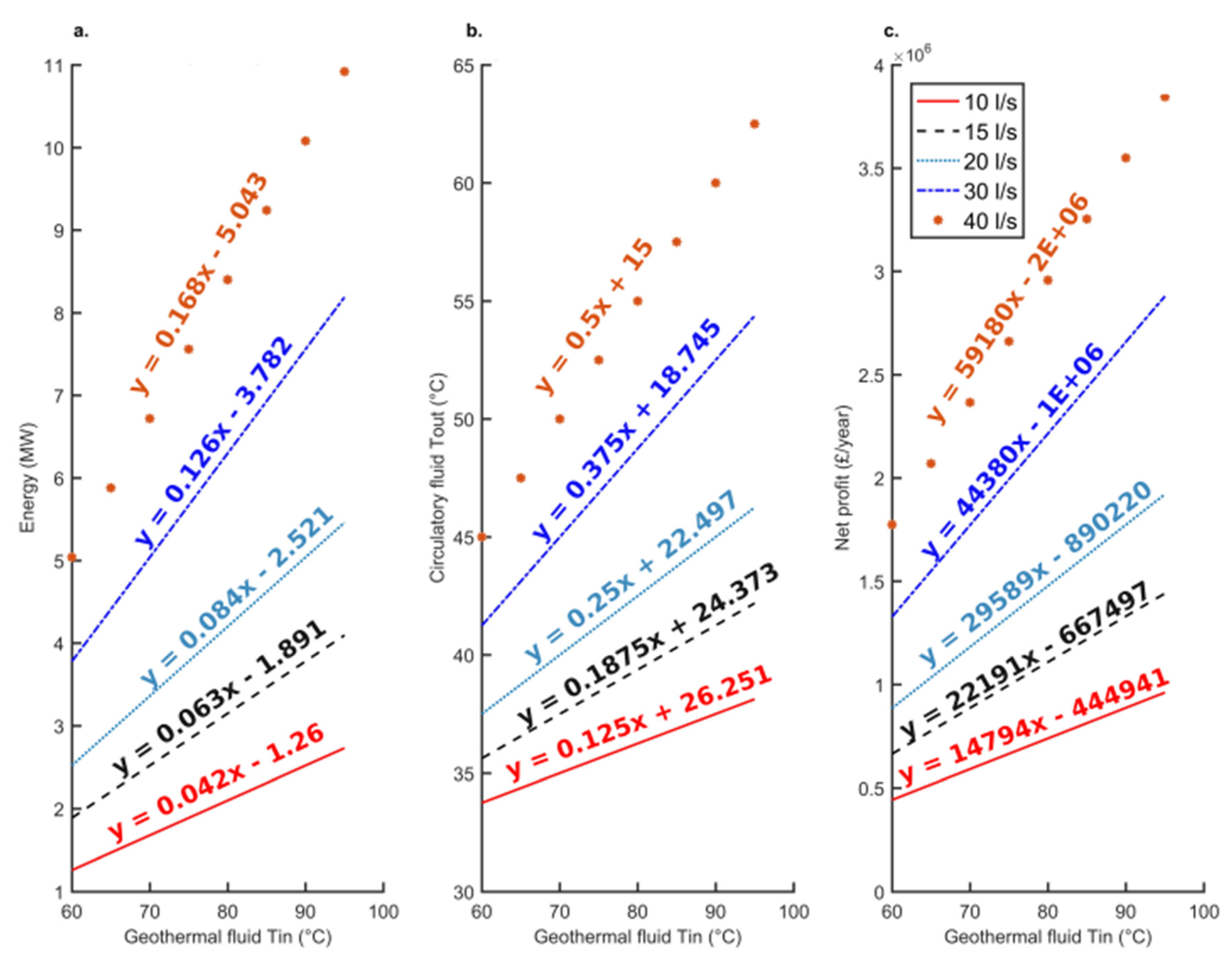
3.3.3. Comparison of Output Temperatures and Regression Models

Optimal surface areas under the lowest heat exchanger costs and interest rates resulted in the output temperatures for the geothermal fluid being 30.0032 °C for both high and low temperature input scenarios. The output temperature of the circulatory fluid was 48.5 °C and 58 °C for the 67 °C and 86 °C input temperatures of the geothermal fluids, respectively.

Further testing was also undertaken for geothermal fluid inlet temperatures of 60 °C to 95 °C, keeping a fixed interest of 0.01 and cost of heat exchanger per unit area of 50 £/m². As was expected, increasing the geothermal fluid input temperature results in greater circulating water output temperatures (Figure 9a); this is observed as a linear trend (Figure 9b,c). In Figure 9b, an exponential trend is observed between the optimal heat transfer area and net profit. Figure 10 highlights the changes in output energy, circulatory fluid, and net profit for different flow rates and temperatures, all of which show a linear increase with increasing geothermal fluid temperature.

4. Discussion

4.1. Implications to Other Geothermal DHN across the UK

In the UK there are several Mesozoic Basins holding hot sedimentary aquifers and several hot dry rock prospects with the potential for deep geothermal schemes supplying heat to a DHN. Although a concentrated demand is required at surface level, the subsurface and geothermal capability will dictate any potential scheme. As such, with known formation temperatures, it is possible to infer potential net profits if a district heat network were to be developed.

The North Pennine Batholith has been explored as a potential source of heat in recent years, with the likelihood it will be used for direct heat use and electricity generation (e.g., [6,33,34]). Recent 3D geological modelling suggests that temperatures of 100 °C can be found at depths of ~3 km ([34]). A doublet scheme, connected by natural [6,35] or un-natural fractures (an enhanced geothermal system), could therefore be used for direct heat use. By considering the regression models developed in this study, the estimated net profit for the lowest 10 L/s flow rate would be £1.0345 million per year. This may not be economic for an enhanced geothermal system. However, if the thermal regime permits, and temperatures in excess of 100 °C are observed, then there is the potential for a cascade scheme (e.g., [36]) to exploit heat for electricity and, subsequently, for a DHN. The North Pennine Batholith also has the benefit of having concentrated demand on the surface for a DHN, with large population densities in areas such as Newcastle and Sunderland.

Additionally, cost savings can be calculated for the Southampton DHN, which is the only deep geothermal-fed DHN in the UK at present. Geothermal energy is exploited at 10–15 L/s ([37,38]) with temperatures of 74 °C recorded ([5]). When calculating the total net savings, this can be equated to £16.245 million over the operational period of 25 years to date (assuming the lower flow rate of 10 L/s). Other selected geothermal prospects in the UK are listed in Table 4, highlighting further potential savings. The table highlights significant savings for a DHN can be made over the lifetime of a project, even with lower temperatures and flow rates.

It has also been suggested that onshore oil wells in the UK could be repurposed for geothermal direct heat use, particularly in the East Midlands Petroleum Province ([39,40,41]). This would reduce costs further, as there would be no capital expenditure spent on drilling a geothermal well, and could make a geothermal scheme economic.

Table 4. Selected geothermal prospects estimated net profit per year.

Location	Temperature (°C)	Depth (km)	Net Profit for 10 L/s Flow Rate (Million £/Year)	Net Profit for 40 L/s Flow Rate (Million £/Year)	Temperature and Depth Reference
North Pennine Batholith (Northeast England)	100	3	1.0345	3.918	[34]
Wessex Basin (Souhampton)	74	1.725	0.6498	2.3793	[5]
Cornubian Granite (Rosemanowes)	90	2.175	0.8865	3.3262	[38]
Larne Basin (N. Ireland)	91	2.873	0.9013	3.3853	[38]

Table 4. Selected geothermal prospects estimated net profit per year.

Location	Temperature (°C)	Depth (km)	Net Profit for 10 L/s Flow Rate (Million £/Year)	Net Profit for 40 L/s Flow Rate (Million £/Year)	Temperature and Depth Reference
North Pennine Batholith (Northeast England)	100	3	1.0345	3.918	[34]
Wessex Basin (Souhampton)	74	1.725	0.6498	2.3793	[5]
Cornubian Granite (Rosemanowes)	90	2.175	0.8865	3.3262	[38]
Larne Basin (N. Ireland)	91	2.873	0.9013	3.3853	[38]

4.2. Regression Analysis Reliability

The regression models can be used in this study to calculate net profit, circulatory fluid output temperature, and energy with strong confidence. The linear fit has a R² value of one, which suggests all the data in the study fits the model. Furthermore, the exponential increase for optimum heat transfer area has a strong fit with R² value 0.99.

4.3. Considering the Cost to Drill a Geothermal Doublet

Drilling deep geothermal wells is costly and can be the greatest expense for a district heating scheme based on geothermal supply. The cost of drilling a well can be calculated according to ([42]):

$$Well cost=1.72\times {10}^{-7}\times {\left(MD\right)}^2+2.3\times {10}^{-3}\times MD-0.62$$

(9)

where MD is depth of the well in metres. The equation gives the well cost in millions of dollars which is converted to pounds using a factor of 0.77.

The cost of drilling a single well in the Cheshire Basin would be in the region of £5.7 million, assuming the reservoir is located at a depth of 2800 m [12,19,20,25] For the worst-case scenario (67 °C input temperature of the geothermal fluid and high heat exchanger cost of £400 m²), the savings of switching to a geothermal run district heat network would be £2.1784 million per year. The payback time for a doublet (two-well) scheme would, therefore, be ~5.2 years. The minimum total savings, including the cost of a geothermal well, would be £43.06 million (assuming a lifetime of 25 years). If the highest amount of savings can be made (86 °C input temperature of the geothermal fluid and a low heat exchanger cost of £50 m²), then the payback time will be under 4 years. The savings over a 25-year lifetime will be £71.5 million.

5. Conclusions

This paper presented a comparative analysis of different heat exchangers for use in a geothermal-fed district heating scheme for the Crewe area, overlying the Cheshire Basin. Counter-flow heat exchangers can produce significant savings, in comparison with fossil fuels, over the lifetime of a heat exchanger (25 years). This includes the drilling cost for a doublet system. Co-current flow heat exchangers were also analysed and it was identified that they had far lower effectiveness.

Based on geothermal temperatures from the literature, the most efficient surface area of the heat exchanger was found to be 727 m² and 762 m² for geothermal fluid input temperatures of 67 °C and 86 °C. This results in total savings of £43.06 million and £71.5 million, respectively. Using an input temperature of 30 °C for the circulatory fluid, the output temperature of the circulating fluid for the lower and higher input geothermal temperatures were 48.5 °C and 58 °C. This would be the likely range of achievable system temperatures that a district heating system could operate under.

Building on this, for a deep geothermal energy scheme in the Cheshire basin, under the best-case scenario (95 °C geothermal fluid temperature and 40 L/s flow rate), a doublet well system could produce 10.92 MW of energy. If coupled to the district heating scheme in Crewe town centre, the initial capital expenditure would be £11.4 million. However, by using a geothermal-fed DHN rather than a conventional fossil-fuelled network, savings of £3.845 million per annum could be made.

For the worst-case scenario (60 °C geothermal fluid temperature and 10 L/s), a doublet scheme could produce 1.26 MW. The capital expenditure would be identical to that of the optimal conditions. The total savings per annum by using a geothermal-fed heat network would be £0.443 million. In this scenario, the geothermal scheme would not recover the initial capital expenditure over the 25-year lifetime.

This study has also determined that any doublet well scheme, when used in conjunction with a heat exchanger, must have flow rates and production temperatures in excess of 10 L/s and 70 °C, respectively, to be viable to meet the Crewe energy demand for phase one of the heat network (1.6 MW). Regression models can also be used to predict net savings for a geothermal-fed DHN in other areas across the UK.

References

1. Björnsson, O.B. Geothermal District Heating. In International Workshop on Direct Use of Geothermal Energy; Chamber of Commerce and Industry of Slovenia: Ljubliana, Slovenia, 1999; Available online: https://geothermalcommunities.eu/assets/elearning/5.16.1999-Geothermal-District-Heating.pdf (accessed on 5 March 2020).
2. Rollin, K.E.; Kirby, G.A.; Rowley, W.J.; Buckley, D.K. Atlas of Geothermal Resources in Europe: UK Revision; Technical Report WK/95/07; British Geological Survey: Nottingham, UK, 1995. [Google Scholar]
3. Hirst, C.M.; Gluyas, J.G.; Adams, C.A.; Mathias, S.A.; Bains, S.; Styles, P. UK Low Enthalpy Geothermal Resources: The Cheshire Basin. In Proceedings of the World Geothermal Congress, Melbourne, Australia, 19–25 April 2015. [Google Scholar]
4. Downing, R.A.; Gray, D.A. Geothermal Energy the Potential in the United Kingdom; BGS, National Environment Research Council: Nottingham, UK, 1986. [Google Scholar]
5. Barker, J.A.; Downing, R.A.; Gray, D.A.; Findlay, J.; Kellaway, G.A.; Parker, R.H.; Rollin, K.E. Hydrogeothermal studies in the United Kingdom. Q. J. Eng. Geol. Hydrogeol. 2000, 33, 41–58. [Google Scholar] [CrossRef]
6. Busby, J.P. Geothermal prospects in the United Kingdom. In Proceedings of the World Geothermal Congress, Bali, Indonesia, 25–29 April 2010. [Google Scholar]
7. Busby, J. Geothermal energy in sedimentary basins in the UK. Hydrogeol. J. 2014, 22, 129–141. [Google Scholar] [CrossRef] [Green Version]
8. Routledge, K.; Williams, J.; Lehdonvirta, H.; Kuivala, J.-P.; Fagerstrom, O. Heat Network Mapping for Leighton West; Report number: 298-692; A Report Prepared for Cheshire East Council; Crewe, UK, 2014. [Google Scholar]
9. Chuanshan, D.; Jun, L. Optimum design and running of PHEs in geothermal district heating. Heat Transf. Eng. 1999, 20, 52–61. [Google Scholar] [CrossRef]
10. Ağra, Ö.; Erdem, H.H.; Demir, H.; Atayılmaz, Ş.Ö.; Teke, İ. Heat capacity ratio and the best type of heat exchanger for geothermal water providing maximum heat transfer. Energy 2015, 90, 1563–1568. [Google Scholar] [CrossRef]
11. Shi, Y.; Song, X.; Li, G.; Li, R.; Zhang, Y.; Wang, G.; Zheng, R.; Lyu, Z. Numerical investigation on heat extraction performance of a downhole heat exchanger geothermal system. Appl. Therm. Eng. 2018, 134, 513–526. [Google Scholar] [CrossRef]
12. Brown, C.S.; Cassidy, N.J.; Egan, S.S.; Griffiths, D. Numerical modelling of deep coaxial borehole heat exchangers in the Cheshire Basin, UK. Comput. Geosci. 2021, 152, 104752. [Google Scholar] [CrossRef]
13. Sliwa, T.; Leśniak, P.; Sapińska-Śliwa, A.; Rosen, M.A. Effective Thermal Conductivity and Borehole Thermal Resistance in Selected Borehole Heat Exchangers for the Same Geology. Energies 2022, 15, 1152. [Google Scholar] [CrossRef]
14. Amanowicz, Ł.; Wojtkowiak, J. Comparison of Single-and Multipipe Earth-to-Air Heat Exchangers in Terms of Energy Gains and Electricity Consumption: A Case Study for the Temperate Climate of Central Europe. Energies 2021, 14, 8217. [Google Scholar] [CrossRef]
15. Mirzaei, M.; Hajabdollahi, H.; Fadakar, H. Multi-objective optimization of shell-and-tube heat exchanger by constructal theory. Appl. Therm. Eng. 2017, 125, 9–19. [Google Scholar] [CrossRef]
16. Khan, T.A.; Li, W. Optimal design of plate-fin heat exchanger by combining multi-objective algorithms. Int. J. Heat Mass Transf. 2017, 108, 1560–1572. [Google Scholar] [CrossRef] [Green Version]
17. Imran, M.; Pambudi, N.A.; Farooq, M. Thermal and hydraulic optimization of plate heat exchanger using multi objective genetic algorithm. Case Stud. Therm. Eng. 2017, 10, 570–578. [Google Scholar] [CrossRef]
18. Dagdas, A. Heat exchanger optimization for geothermal district heating systems: A fuel saving approach. Renew. Energy 2007, 32, 1020–1032. [Google Scholar] [CrossRef]
19. Brown, C.S.; Cassidy, N.; Egan, S.; Griffiths, D. Modelling low-enthalpy deep geothermal reservoirs in the Cheshire Basin, UK as a future renewable energy source. In Proceedings of the AAPG Annual Convention and Exhibition, San Antonio, TX, USA, 19–22 May 2019; Volume 21. [Google Scholar]
20. Brown, C.S.; Cassidy, N.; Egan, S.; Griffiths, D. Evaluating the response of geothermal reservoirs in the Cheshire Basin: A parameter sensitivity analysis. In Proceedings of the AAPG Annual Convention and Exhibition, San Antonio, TX, USA, 19–22 May 2019. [Google Scholar]
21. Westaway, R. Deep Geothermal Single Well heat production: Critical appraisal under UK conditions. Q. J. Eng. Geol. Hydrogeol. 2018, 51, 424–449. [Google Scholar] [CrossRef]
22. Bradley, J.C. Counterflow, crossflow and cocurrent flow heat transfer in heat exchangers: Analytical solution based on transfer units. Heat Mass Transf. 2010, 46, 381–394. [Google Scholar] [CrossRef]
23. Plant, J.A.; Jones, D.G.; Haslam, H.W. (Eds.) The Cheshire Basin: Basin Evolution, Fluid Movement and Mineral Resources in A Permo-Triassic Rift Setting; British Geological Survey: Nottingham, UK, 1999. [Google Scholar]
24. Busby, J. UK Data for Geothermal Resource Assessments. Presentation. Available online: http://egec.info/wpcontent/uploads/2011/09/UK-deep-geothermalresources_JBusby.pdf (accessed on 17 June 2019).
25. Brown, C.S.; Cassidy, N.J.; Egan, S.S.; Griffiths, D. A sensitivity analysis of a single extraction well from deep geothermal aquifers in the Cheshire Basin, UK. Q. J. Eng. Geol. Hydrogeol. 2022. [Google Scholar] [CrossRef]
26. Haghighi, A.; Pakatchian, M.R.; Assad, M.E.H.; Duy, V.N.; Alhuyi Nazari, M. A review on geothermal Organic Rankine cycles: Modeling and optimization. J. Therm. Anal. Calorim. 2021, 144, 1799–1814. [Google Scholar] [CrossRef]
27. Zhu, J.; Zhang, W. Optimization design of plate heat exchangers (PHE) for geothermal district heating systems. Geothermics 2004, 33, 337–347. [Google Scholar] [CrossRef]
28. Zarrouk, S.J.; Woodhurst, B.C.; Morris, C. Silica scaling in geothermal heat exchangers and its impact on pressure drop and performance: Wairakei binary plant, New Zealand. Geothermics 2014, 51, 445–459. [Google Scholar] [CrossRef]
29. Teke, I.; Ağra, Ö.; Atayılmaz, Ş.Ö.; Demir, H. Determining the best type of heat exchangers for heat recovery. Appl. Therm. Eng. 2010, 30, 577–583. [Google Scholar] [CrossRef]
30. Ağra, Ö. Sizing and selection of heat exchanger at defined saving–investment ratio. Appl. Therm. Eng. 2011, 31, 727–734. [Google Scholar] [CrossRef]
31. Annamalai, K.; Puri, I.K. Combustion Science and Engineering; CRC Press: Boca Raton, FL, USA, 2006. [Google Scholar]
32. BOE. Available online: https://www.bankofengland.co.uk/ (accessed on 8 August 2021).
33. Manning, D.; Younger, P.; Smith, F.; Jones, J.; Dufton, D.; Diskin, S. A deep geothermal exploration well at Eastgate, Weardale, UK: A novel exploration concept for low-enthalpy resources. J. Geol. Soc. 2007, 164, 371–382. [Google Scholar] [CrossRef]
34. Howell, L.; Brown, C.S.; Egan, S.S. Deep geothermal energy in northern England: Insights from 3D finite difference temperature modelling. Comput. Geosci. 2021, 147, 104661. [Google Scholar] [CrossRef]
35. Younger, P.L.; Gluyas, J.G.; Stephens, W.E. Development of deep geothermal energy resources in the UK. Proc. Inst. Civ. Eng. -Energy 2012, 165, 19–32. [Google Scholar] [CrossRef]
36. Rubio-Maya, C.; Díaz, V.A.; Martínez, E.P.; Belman-Flores, J.M. Cascade utilization of low and medium enthalpy geothermal resources—A review. Renew. Sustain. Energy Rev. 2015, 52, 689–716. [Google Scholar] [CrossRef]
37. Smith, M. Southampton energy scheme. In World Geothermal Congress; IGA: Tokyo, Japan, 2000. [Google Scholar]
38. Gluyas, J.G.; Adams, C.A.; Busby, J.P.; Craig, J.; Hirst, C.; Manning, D.A.C.; McCay, A.; Narayan, N.S.; Robinson, H.L.; Watson, S.M.; et al. Keeping warm: A review of deep geothermal potential of the UK. Proc. Inst. Mech. Eng. Part A J. Power Energy 2018, 232, 115–126. [Google Scholar] [CrossRef] [Green Version]
39. Hirst, C.M.; Gluyas, J.G. The geothermal potential held within Carboniferous sediments of the East Midlands: A new estimation based on oilfield data. In Proceedings of the World Geothermal Congress, Melbourne, Australia, 19–25 April 2015; Available online: https://www.geothermal-energy.org/pdf/IGAstandard/WGC/2015/16079.pdf (accessed on 25 June 2020).
40. Hirst, C.M.; Gluyas, J.G.; Mathias, S.A. The late field life of the East Midlands Petroleum Province: A new geothermal prospect? Q. J. Eng. Geol. Hydrogeol. 2015, 48, 104–114. [Google Scholar] [CrossRef] [Green Version]
41. Watson, S.M.; Falcone, G.; Westaway, R. Repurposing hydrocarbon wells for geothermal use in the UK: The onshore fields with the greatest potential. Energies 2020, 13, 3541. [Google Scholar] [CrossRef]
42. Lukawski, M.Z.; Anderson, B.J.; Augustine, C.; Capuano, L.E., Jr.; Beckers, K.F.; Livesay, B.; Tester, J.W. Cost analysis of oil, gas, and geothermal well drilling. J. Pet. Sci. Eng. 2014, 118, 1–14. [Google Scholar] [CrossRef]
Figure 1. Schematic of geothermal system supplying a district heat network (DHN).
Energies 15 01983 g001
Figure 2. Map of the UK highlighting the study area and location of the Cheshire Basin.
Energies 15 01983 g002
Figure 3. Different types of heat exchanger configurations, including co-current flow and counter-current flow regimes. Tc is the temperature of the circulatory fluid and Th is for the geothermal fluid. The addition of ‘out’ and ‘in’ refer to the inlet or outlet temperatures.
Energies 15 01983 g003
Figure 4. (a) Different outlet temperatures for counter-current and (b) different outlet temperatures for co-current flow heat exchangers across a range of heat transfer areas, with their respective efficiencies (c). The input temperature for the geothermal fluid was 86 °C.
Energies 15 01983 g004
Figure 5. (a) Different outlet temperatures for counter-current and (b) different outlet temperatures for co-current flow heat exchangers across a range of heat transfer areas, with their respective efficiencies (c). The input temperature for the geothermal fluid was 67 °C.
Energies 15 01983 g005
Figure 6. Varying net profit and capital investment versus heat transfer area for different input geothermal temperatures (a) 67 °C and (b) 86 °C. The optimal surface area is the maximum difference between these two values.
Energies 15 01983 g006
Figure 7. Varying net profit versus heat transfer area for different heat exchanger costs (a) and interest rates (b). The input temperature of the geothermal fluid was 67 °C and the clean circulating fluid was 30 °C.
Energies 15 01983 g007
Figure 8. Varying net profit versus heat transfer area for different heat exchanger costs (a) and interest rates (b). The input temperature of the geothermal fluid was 86 °C and the circulating fluid was 30 °C.
Energies 15 01983 g008
Figure 9. (a) Change in geothermal fluid and circulating fluid output temperatures for different heat exchanger transfer areas across the 60–95 °C input geothermal fluid temperature range; (b) variation in net profit and optimal transfer area as a consequence of changes in input temperature of the geothermal fluid; and (c) variation in output of circulating fluid in comparison with the geothermal fluid input temperature.
Energies 15 01983 g009
Figure 10. Variation in energy (a), circulatory fluid output temperature (b), and net profit (c) with changes in geothermal fluid flow rate. Note the R2 values are one for all regression equations.
Energies 15 01983 g010