Abstract
Correlations for the Nusselt number for the fully-developed laminar flow of Carreau fluids through circular pipe subject to a uniform heat flux have been sought. Based on the mathematical expression, the Nusselt number could be obtained by numerical integration. To evaluate the Nusselt number for many conditions, an efficient integration method has been proposed. Using the obtained Nusselt number for different material constants and flow conditions, an improved correlation method has been proposed. The proposed correlation could reduce the maximum error from 3% to 0.9%.
1. Introduction
The convective laminar fully-developed flow through a circular tube has been a basic element in heat transfer engineering. Especially for non-Newtonian fluids, it requires complicated analyses, even for laminar flows [1,2]. The convective heat transfer of non-Newtonian fluids takes place in flows of blood, polymeric liquids, slurries, and so on. For the uniform heat flux and temperature conditions, the heat transfer coefficient is constant for a Newtonian and power-law fluid as long as the laminar condition is maintained. However, for other non-Newtonian fluids, the heat transfer coefficient can vary along with the flow condition. Especially in many polymer and slurry processes, temperature variation is important to control the process conditions. In earlier studies, it has been found that the Nusselt number increases from the Newtonian value to the power law value for nonlinear shear-thinning models without truncation [3]. In this case, the transition is a smooth ramping-up along with the shear rate [4]. However, with the truncation, the Nusselt number changes over a wide range of shear rates, resulting in a nonlinear curve with a rise and fall [5]. Although the power law model is still employed in heat transfer analyses for complicated geometries [6,7] or physical circumstances [8], modern heat transfer engineering requires more accurate Nusselt numbers.
To obtain a more accurate value of the Nusselt number for a given flow of complicated non-Newtonian fluids, one can obtain the value by a numerical calculation, from tables or graphs in existing works, or using an approximate formula. The Nusselt numbers for various types of conduits have been numerically evaluated for different non-Newtonian models. For example, tubes under the uniform heat flux [5] and uniform temperature [9], slits under the uniform heat flux [10], and rectangular ducts under uniform heat flux and temperature [11] have been investigated. A fully developed flow in tube is governed by a nonlinear ordinary differential equation. Since no time marching is necessary, the numerical procedure seems simple. However, it still requires iterations to resolve the nonlinearity. Moreover, the value should be acquired when the mesh refinement no longer changes the solution. In other words, mesh convergence should be achieved.
An approximate method using the apparent index was proposed for the tube flow and the slit flow [5,12]. In this method, the results were verified by comparison with the numerical results. The method was beneficially applied to various constitutive equations. In particular, the results for the Carreau-Yasuda model [13], which is inclusive of the Cross model [14] and the Carreau models [15], were presented in [5]. A further rheological explanation of those models can be found in [16,17]. Although the approximate results are close to those of the numerical method, significant bias can also be observed. Recently, it has been shown that the Nusselt number under the uniform heat flux condition (UHF) can be obtained for tube flow of the Carreau model only by numerical integration without any numerical method such as the finite difference and finite element methods. This was facilitated by a semi-analytical method in the shear rate domain. Using this method, it is possible to quickly obtain the Nusselt numbers in many cases with different model constants.
This work attempts to improve the accuracy of the existing apparent index method [12] by introducing a modified functional form. Moreover, the semi-analytical method has been employed to determine the coefficients reliably. Earlier, this method was proposed in [1] and applied to the flow modeling of polymer processing [18]. Later, described again in [19] and more recently, it has been applied to the evaluation of friction factors [20] and heat transfer coefficients [5,12]. Although the demand for the correlations for the tube is high, it is difficult to find correlations with improved accuracy.
In this work, the apparent index method is modified by correcting the shear rate and the truncation term following the index of the Carreau model. Moreover, to determine the model coefficients, the semi-analytical method has been employed instead of the numerical method for solving a differential equation. This work utilizes an adaptive quadrature-based integration method, which is described in detail later. This allows reliable and fast estimations of the Nusselt number for various cases. To validate the proposed method, the result is also compared with that in the previous work.
2. Formulation
2.1. Flow
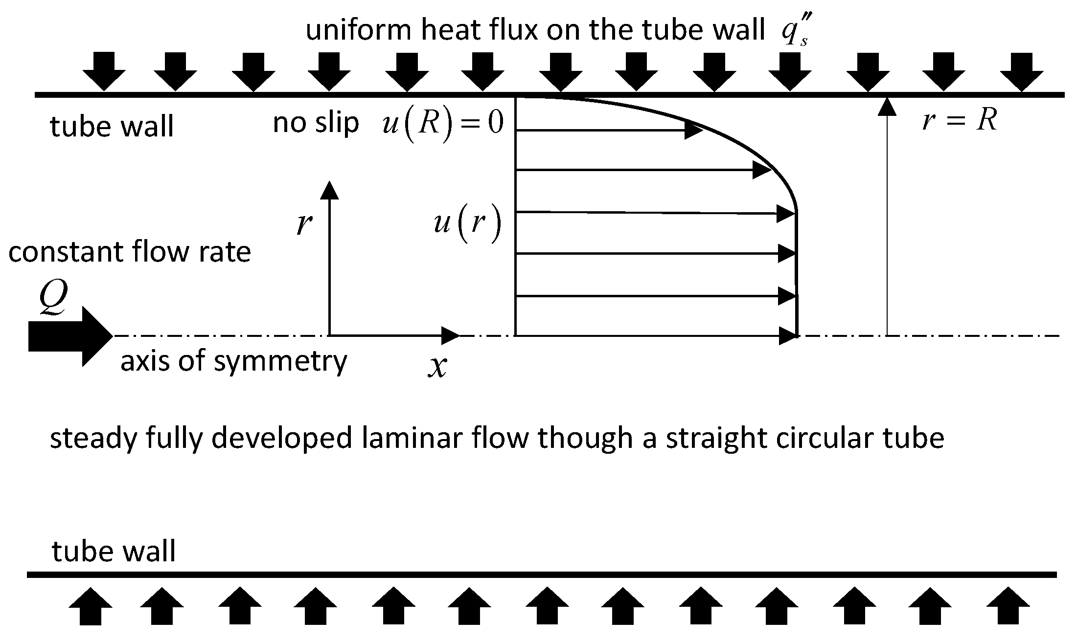
Consider a fully-developed laminar flow through a circular tube shown in Figure 1. A velocity profile is expressed as because of the fully developed condition, . Moreover, the no-slip condition, , is imposed on the tube wall. The total flow rate, Q, is specified.
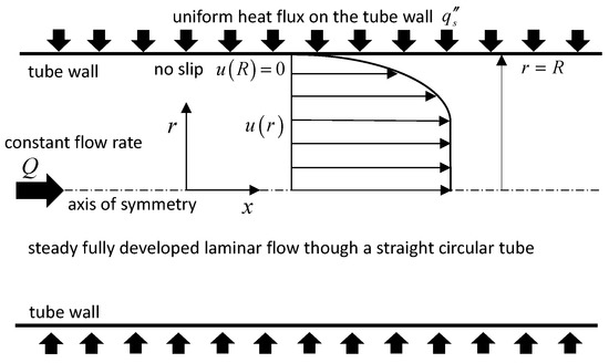
Figure 1.
Outline of the fully-developed flow subject to the uniform heat flux in a circular tube.
2.2. Temperature
In this section, the expressions for the velocity and the flow rate are derived based on the shear rate instead of the position variable [21]. The core flow rate is defined here, and its mathematical form is derived using the expressions for the velocity and the flow rate.
The energy equation for temperature field, , in the fully developed laminar regime without heat generation is of the form [21]
where , , and k are the mean temperature, density, heat capacity, and thermal conductivity, respectively. The energy balance under the uniform wall heat flux of , shown in Figure 1, gives .
2.3. Nusselt Number
Let us introduce the core flow rate, , which is given by
Note that the total flow rate can be described using the above expression as . Taking constant , and k, integration of Equation (1) from 0 to r gives . Then, integration from r to R gives , where is the surface temperature given by . The mean temperature of a fully-developed flow is defined as . With integration by parts followed by suitable arrangements yields . With the definition of heat transfer coefficient, , it is obtained as where the flow rate is given by . Then, the Nusselt number is expressed as [22]
Once is obtained, the Nusselt number can be evaluated right away by integration. Note that viscous heating is ignored in Equation (3) and refer to previous work for the Brinkman number [10,23].
2.4. Evaluation of the Core Flow Rate
To evaluate the Nusselt number by Equation (3), the core flow rate should be evaluated for the corresponding constitutive equation. Integration in Equation (2) can be analytically available when is in a simple form as in the Newtonian or power law fluid. For a Newtonian fluid with a mean velocity of , the velocity is well-known as , then the core flow rate is obtained as
Note that is and should be obtained for any constitutive model. Consider a power law fluid with , where K is the consistency and n is the index. This is a basic viscosity model that expresses the shear thinning in which the viscosity decreases as the shear rate increases. Here, the velocity is is obtained. Then, the core flow rate is
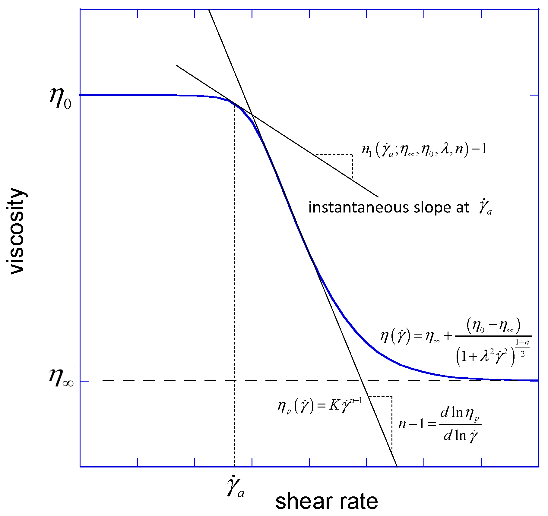
Note that the power law model assumes that the shear thinning takes place over the entire range of the shear rate. In many non-Newtonian fluids such as polymeric liquids, shear thinning occurs at a certain shear rate and weakens at a higher shear rate, as shown in Figure 2. To describe this, a more complicated model is required. However, it is not simple to obtain the core flow rate for complicated models such as the Carreau and Cross. In this case, the evaluation of the core flow rate can be circumvented via the shear stress, and the shear rate, . In tubes, using and , the space variable r and the velocity u can be rewritten again with and . Note that is the wall shear stress corresponding to the wall shear rate . Then, by integration by parts of Equation (2), the core flow rate can be expressed as [21,24],
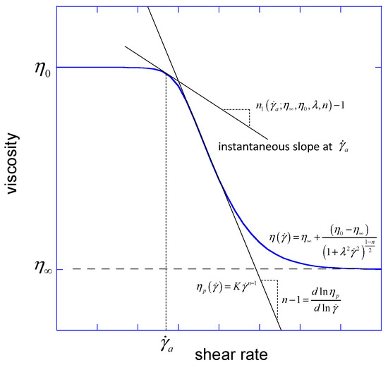
Figure 2.
The Carreau viscosity model and concept of n1.
For the Carreau fluid, the viscosity is of the form
where , and are the viscosity at the infinite shear rate, the zero-shear viscosity, and the time constant, respectively. Figure 2 shows along with together with with the same n.
The Carreau model accommodates the zero-shear viscosity and truncates the viscosity at the large . Without the truncation term, converges to with the same n as increases. Then, using the constitutive equation of the generalized Newtonian fluid, , the core flow rate of the Carreau fluid is obtained as
where the wall shear rate is given by . Similar integrations based on the shear rate are found in [21,22,24].
2.5. Evaluation of the Nusselt Number
The Nusselt number can be easily evaluated for the Newtonian fluid by substituting Equation (4) in Equation (3).
Similarly, for the power law fluid, the Nusselt number is obtained by substituting Equation (5) in Equation (3) gives
It is notified here that Equation (10) will be used to evaluate the Nusselt number of the Carreau model by substituting the apparent power law index.
It is not simple to evaluate Nu for a complex model like the Carreau model. Please, read this paragraph carefully. It should be emphasized that integration can be achieved by changing the integral variable in Equation (3) from r to via . Moreover, the identities, and should be utilized [21]. Using these properties, the substitution of Equation (8) into Equation (3) can give the Nusselt number. Unfortunately, analytically achieving the integral, with the core flow rate given by Equation (8) is not very beneficial because a huge number of terms are generated. Inevitably, this integration should be performed numerically. Moreover, the wall shear rate should be determined for a given by solving a nonlinear algebraic equation, using Equation (8). Nonetheless, it is still advantageous to obtain the Nusselt number using Equation (3) compared to the finite element or the finite difference methods since the solution of a matrix system, and the mesh error can be avoided.
2.6. Numerical Integration
In this work, the numerical integration is fulfilled by the Cuhre algorithm using the cubature rules [25], which is iterative and adaptive though the resulting value is deterministic. With this algorithm, the integration is done by a quadrature rule as follows:
The whole integration interval is subdivided as required. When applying the quadrature, the subdivision becomes smaller near the problematic points. The procedure is as follows [26]:
- (1)
- Further divide a subdomain with the largest predicted error.
- (2)
- Apply a cubature rule to the new subdomain.
- (3)
- Update the integral in the subdomains and obtain the global integral.
- (4)
- Check the error by
Acknowledge that the integration in the subdomain is recursively conducted in a nested way.
2.7. Expressions for Correlations
Assuming a Newtonian flow, the apparent shear rate is described as
Then, the apparent viscosity is obtained by
The Carreau fluid renders a viscosity curve shown in Figure 2. As shown in the figure, the viscosity behaves like a Newtonian fluid in the low shear rate regime and like a power law one in the high shear regime. For the power law model, the following identity holds
It should be noted that both and are functions only of n independent of K. Based on this idea, a method has been proposed to utilize this property even in more complex models. In this method, the original Carreau model can be approximated to a power law form by [1,5]
As mentioned, is not considered an approximate evaluation of Nu; is the only function of interest. In consideration of Equation (14), the apparent index for a specific that characterizes the flow can be proposed as
For a Carreau fluid, the above relation can be written again as
where φ and are defined as and , respectively.
Placing the above quantity into Equation (10) gives an approximate Nusselt number, . In other words, the change from zero shear rate to the wall shear rate is approximated by a result of substituting the value of n1 at the apparent shear rate into . Since the velocity profiles of the power law and the Carreau model are different from each other, the core flow rates would be different, and thus the Nusselt number would be so also. Thus, the mathematical foundation of the method seems weak and is thought to be a phenomenological methodology. Although the bias from the accurate value is somewhat noticeable, this method efficiently yields a useful number. This will be examined later in this work. To overcome the bias, this work modifies . The modified apparent index takes the form of
where , and are real numbers that are functions of . Then, becomes an input to Equation (10) instead of , which means Nu is evaluated by . The reason for modification of is that the adoption of the apparent shear rate is simply a convention and the corresponding physical background is weak. Thus, is replaced by to improve the accuracy. Moreover, since the Nusselt number variation is known to change dramatically alongside , it is modified by a function as . Based on the solutions in Equation (3), , and will be sought to provide an accurate correlation for the Nusselt number of the Carreau fluid.
3. Results
3.1. Evaluation of Nusselt Number
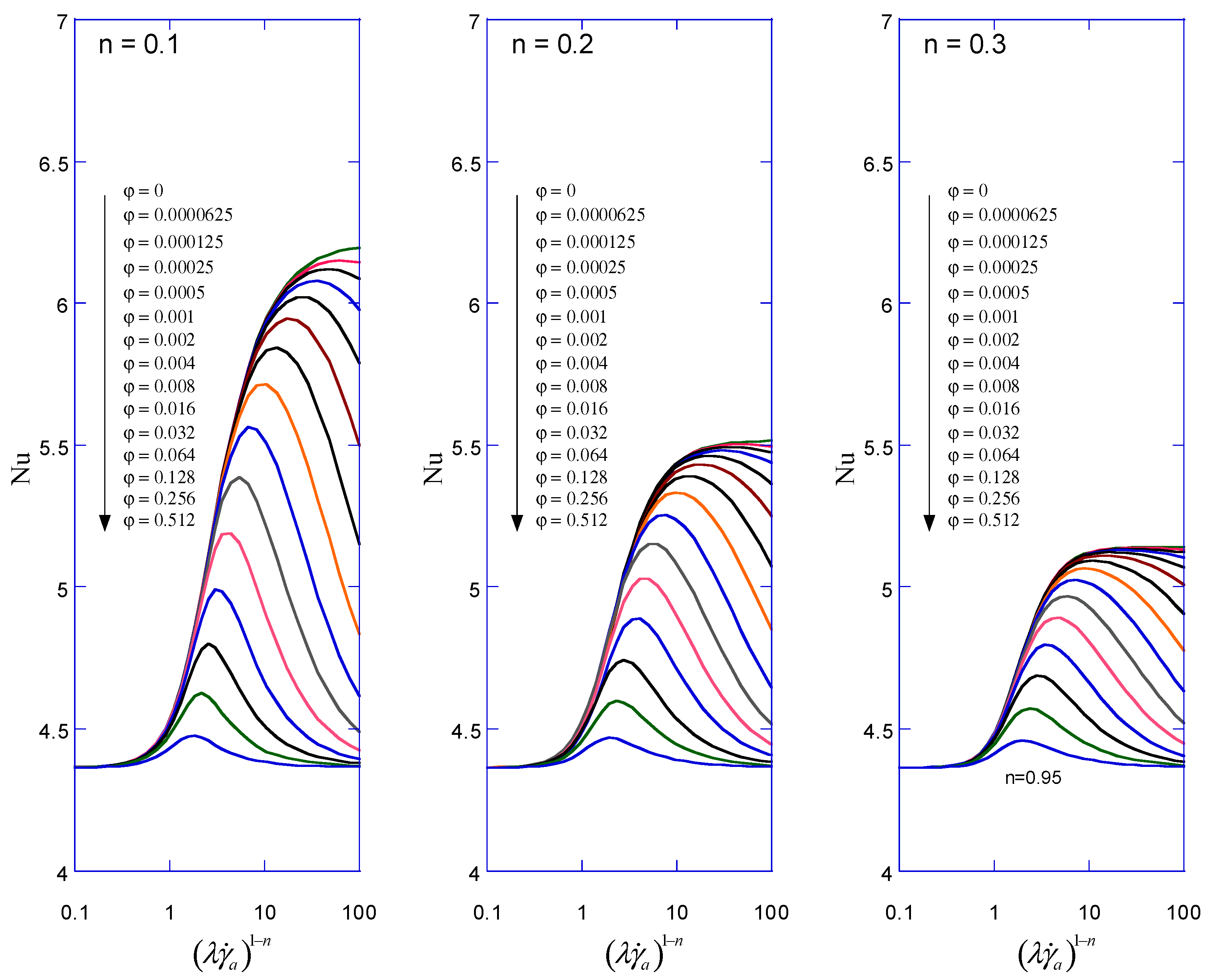
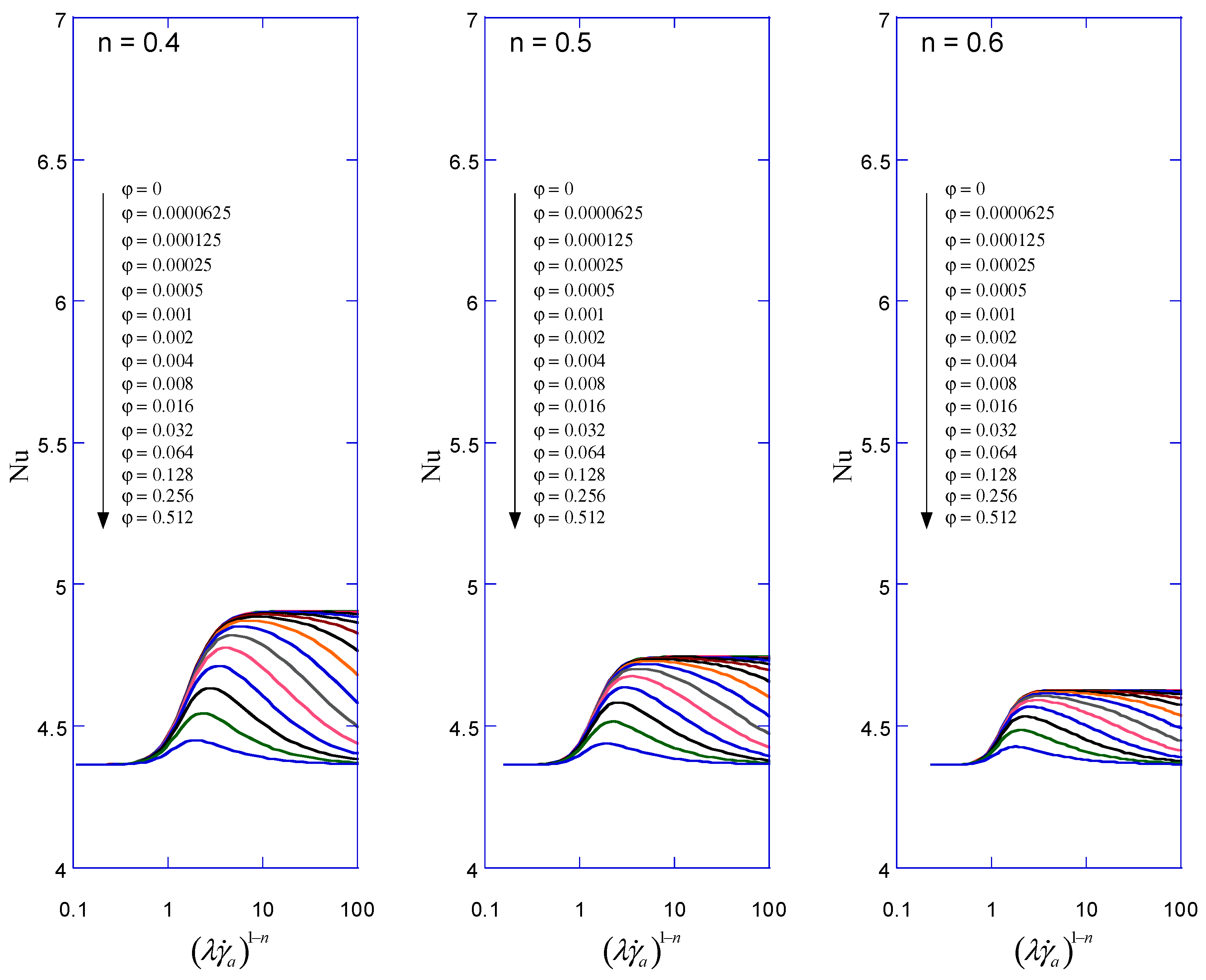
Let us first demonstrate evaluated Nu for various viscosity constants. As aforementioned, the evaluation of Nu is quite straightforward. Putting Equation (8) into Equation (3) followed by numerical integration gives the number. The benefit of this approach is that Nu for many different conditions can be easily and rapidly obtained. This work presents Nu for for . For each n, Nu is obtained for for . Since n is more crucial to evaluation of Nu, a finer discretization has been give for n. It is known that Nu for different n can be presented in a similar range of [10]. All these calculated values of Nu will be put into determining the correlation.
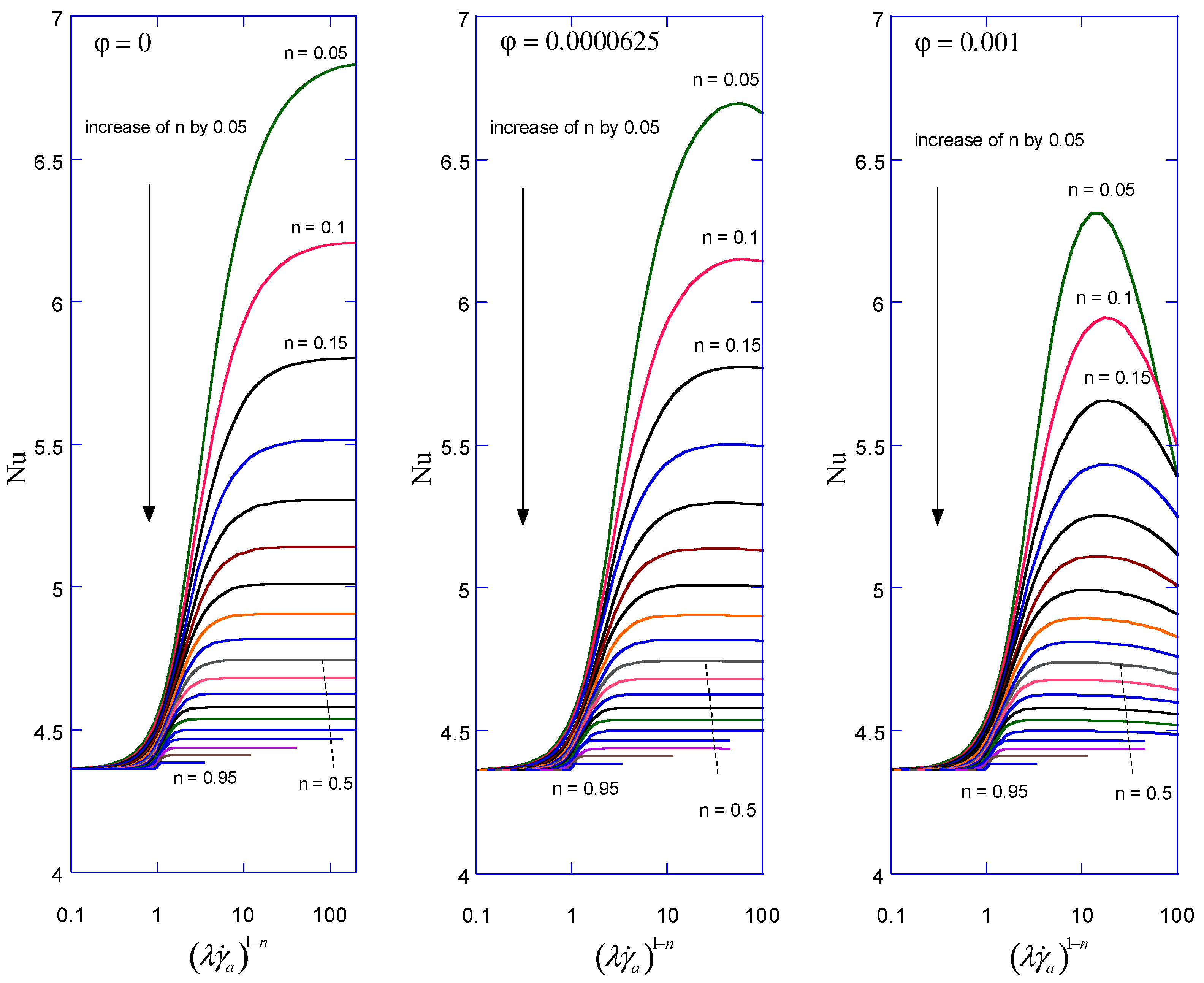
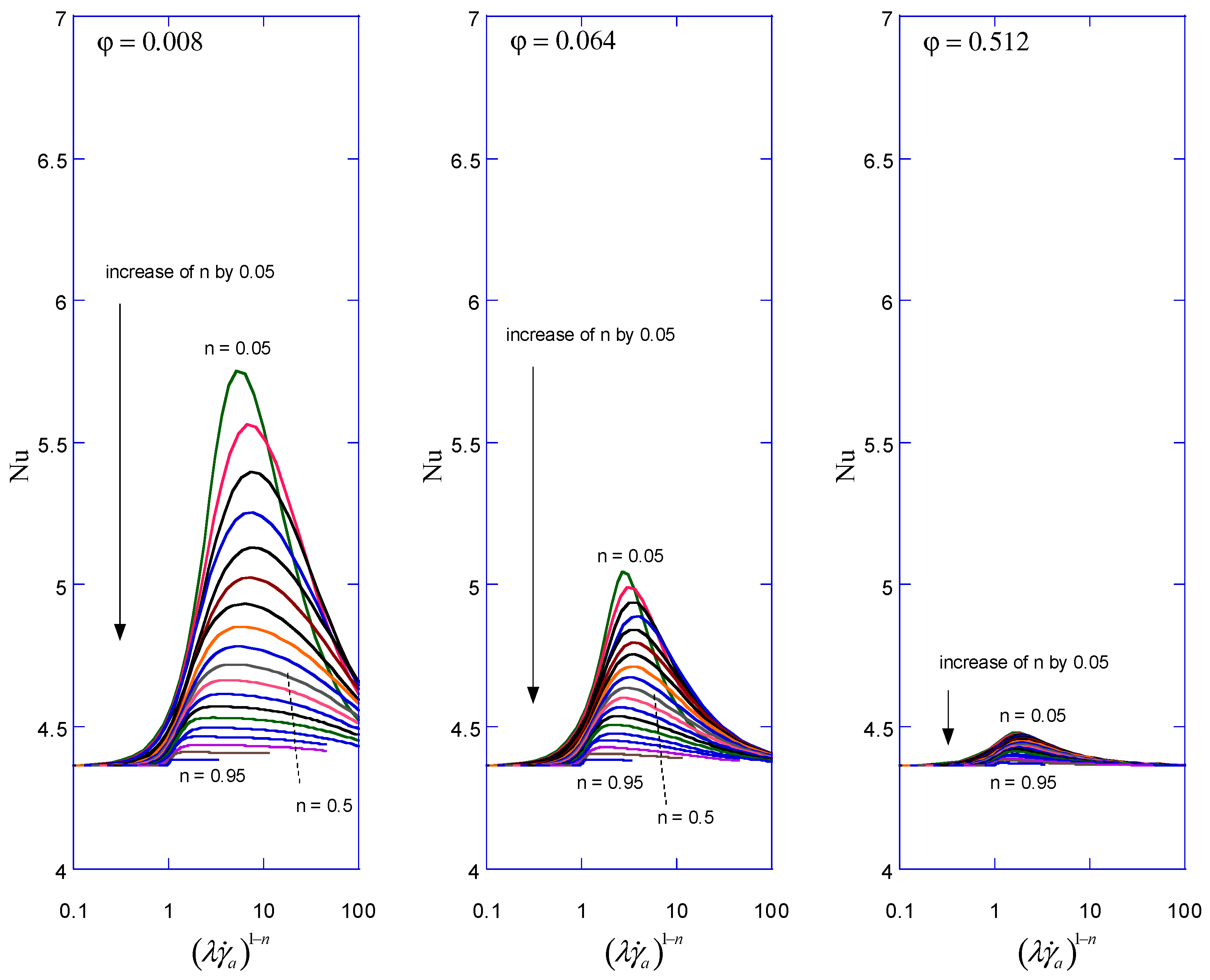
Figure 3 shows Nu for alongside for = 0, 0.0000625, 0.001, 0.008, 0.016, 0.064 and 0.512. For Nu smoothly ramps up from to as can be seen in the figure. For, Nu peaks out at a point and comes back to . The peak value is not over and depends on and n. As increases, the peak value becomes smaller. As a result, the overall variation alongside the shear rate becomes insignificant. Similar results can also be found in [10,12,22]. Figure 4 shows the evaluated Nu alongside for a given n. For a given n, the overall Nu curve comes down toward as increases, as shown in the figure. Overall, the variation of Nu is pronounced for smaller n and larger . Especially for a moderate range of , < 0.01, such variation can cause significant errors in the estimation of Nu by correlation.
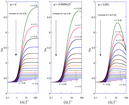
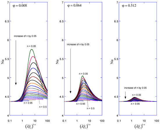
Figure 3.
Nu for alongside for various .
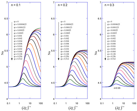
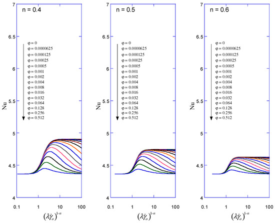
Figure 4.
Nu for alongside for various .
3.2. Correlations
The Nusselt numbers along with from 10−3 to 108 for all the combinations of 19 n’ and 15 ’s. An optimization problem seeking , and that minimizes a sum of least squares
where for . Note that and are defined in the previous section. As a result, a total of 12,825 evaluations of Nu have been conducted to evaluated to set . This work proposes and in Equation (18) as functions of n. Both c and d are expressed as linear functions, which are and . Since h should accommodate severe nonlinearity, it is expressed as h. Then, to determine , and by minimizing Equation (18), the generalized reduced gradient method has been employed. As a result, the following has been achieved:
As a result, for a given set of and , the modified apparent index can be determined by putting Equations (19)–(21) into Equation (18). Then, the Nusselt number is obtained by Equation (10). The results are summarized in Table 1.

Table 1.
Correlation.
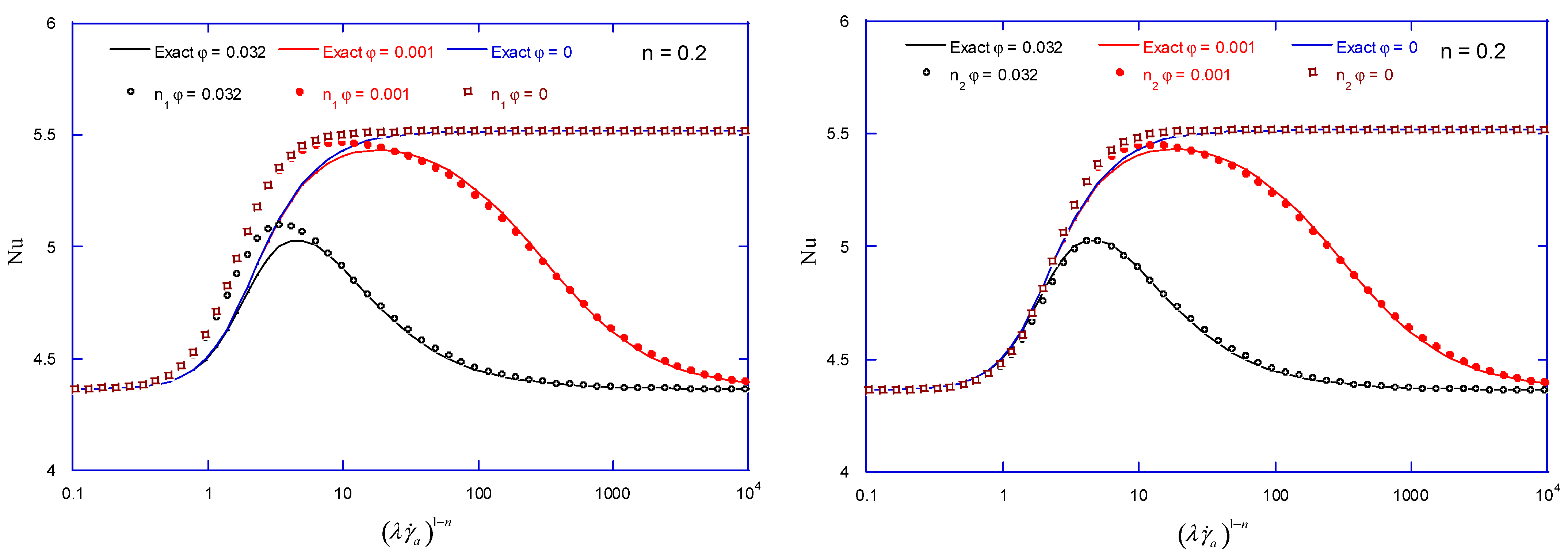
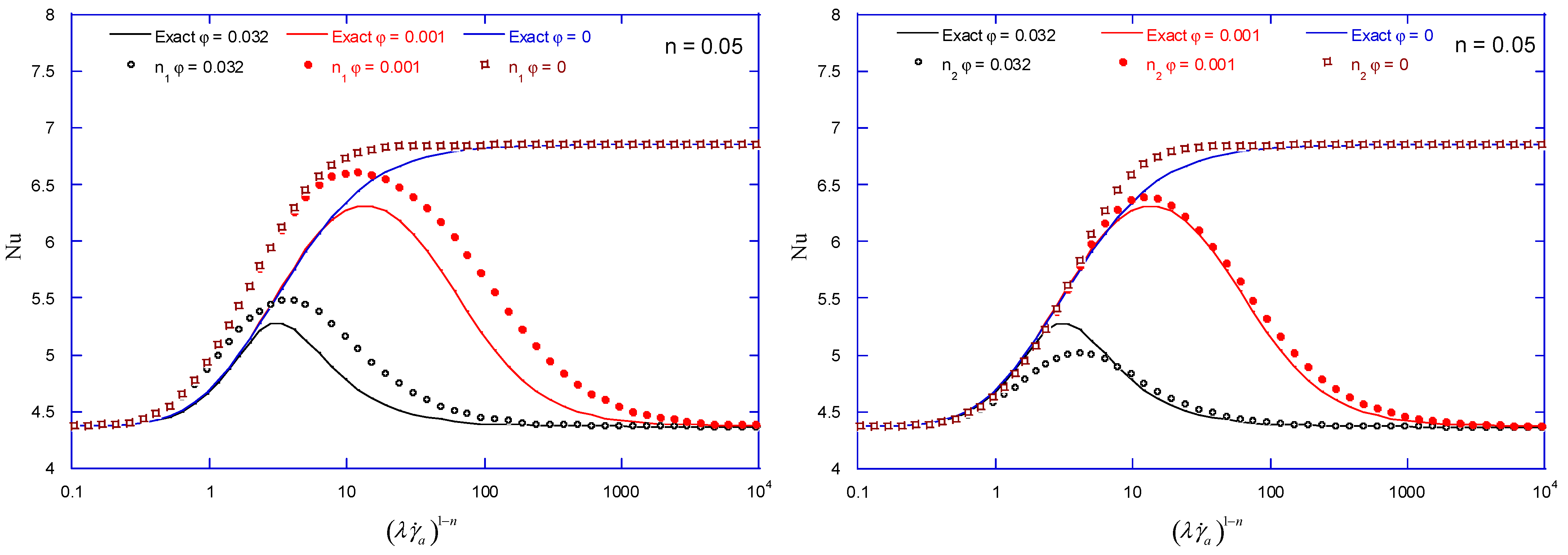
Figure 5 compares Nu values for n = 0.2 with φ = 0, 0.001 and 0.032 by the original apparent index n1 and the modified apparent index n2. With n1, the bias is quite noticeable in the rising edge, but it is significantly reduced by n2. For n = 0.05, the bias is further pronounced with n1, as shown in Figure 6, since the nonlinearity is augmented with the lower n. Again, the bias has been much reduced by n2. Thus, the proposed modified method improves on the accuracy of the original method.
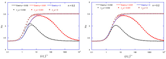
Figure 5.
Nu by n1 and n2 and Equation (3) for n = 0.2.
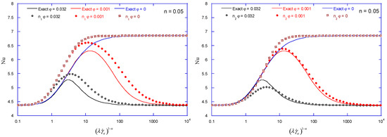
Figure 6.
Nu by n1 and n2 and Equation (3) for n = 0.05.
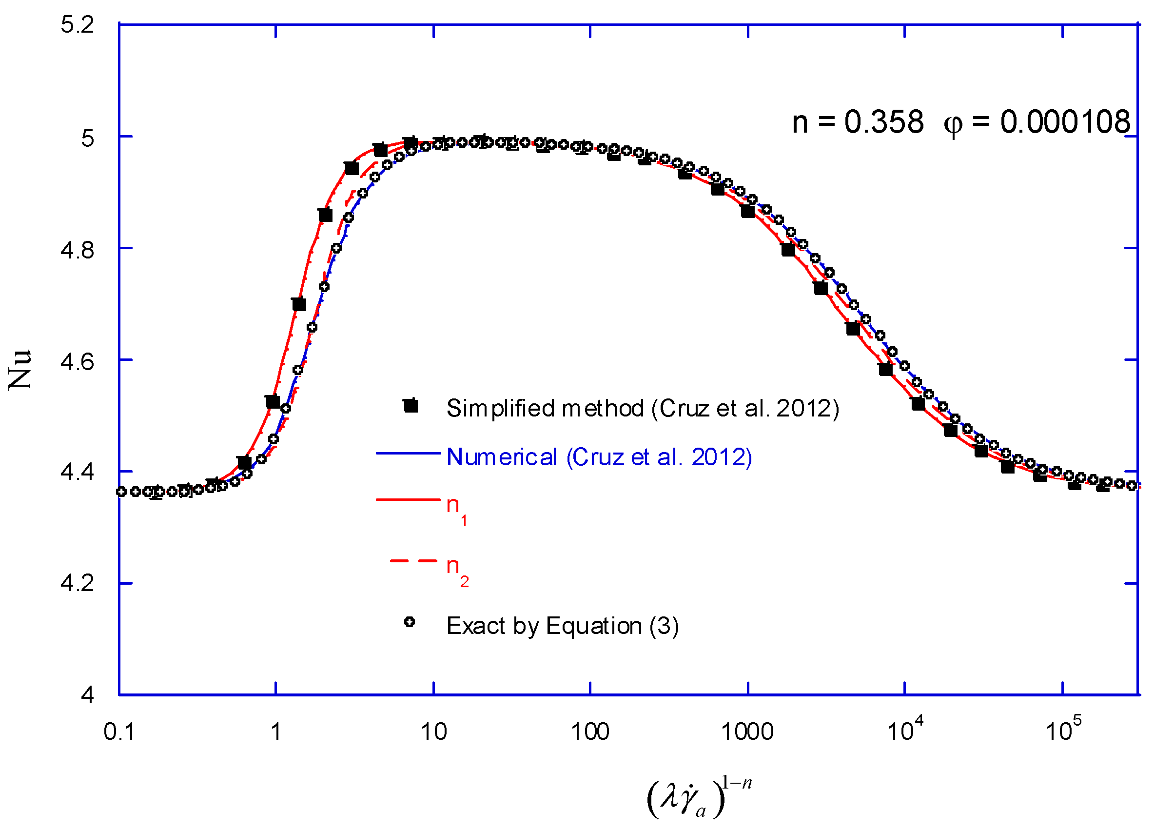
Figure 7 compares the modified method with the data in the original study [5]. The simplified method by Cruz et al. matches the result by n1 in this study. The Nu in Equation (3) and the numerical result by Cruz et al. also agree very well. The bias between them is less pronounced thanks to increased n compared to those in Figure 5 and Figure 6. As can be seen in Figure 7, the result using n2 can reduce the bias dramatically. The maximum error is 3% by n1 and is reduced to 0.9% by n2.
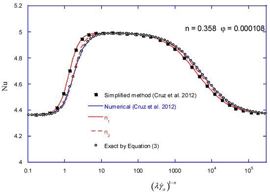
Figure 7.
Nu by n2 and Equation (3) for n = 0.358 and φ = 0.000108.
4. Conclusions
This work has proposed a correlation for Nusselt number for the fully-developed laminar flow of the Carreau fluid in straight tubes. A modified form of the apparent index has been proposed to improve the accuracy of the correlation. On the other hand, thanks to an integration-ready form using the core flow rate, the Nusselt number could be rapidly evaluated for many cases. Based on the obtained results, the constants for the modified apparent index have been determined by optimization. The correlation has been validated by comparing the obtained Nu values with those by the integral formula. Moreover, it has been found that the proposed method can significantly reduce the bias in the original apparent power law index method. The error in Nu estimation has been reduced to 0.9%.
This work considers the Carreau model only, but the modification can be applied to other similar non-Newtonian models. This approach can also be applied to the correlations for pressure drops. In future studies, the modified apparent method needs to be applied to various correlations for Nusselt numbers and friction factors in a unified way.
Funding
This work was supported by NRF grants funded by the Korean government (No. NRF-2018R1A5A1024127 and NRF-2020R1I1A2065650).
Institutional Review Board Statement
Not applicable.
Informed Consent Statement
Not applicable.
Conflicts of Interest
The author declares no conflict of interest.
Nomenclature
| heat capacity | |
| c(n) | function for apparent index modification |
| d | function for apparent index modification |
| h | heat transfer coefficient |
| h | function for apparent index modification |
| p-th evaluation of the integral by the quadratue | |
| k | thermal conductivity |
| K | consistency of the power law model |
| n | index of the viscosity model (a constant of Carreau model) |
| apparent power law index | |
| modified apparent power law index | |
| Nu | Nusselt number |
| Nusselt number for the Newtonian model | |
| Nusselt number for the power law model | |
| core flow rate | |
| core flow rate for Newtonian model | |
| core flow rate for power law model | |
| core flow rate for Carreau model | |
| uniform wall heat flux | |
| Q | flow rate |
| R | radius |
| r | radial position |
| S | sum of least squares |
| T | temperature |
| mean temperature | |
| surface temperature | |
| u | velocity in the x-direction |
| mean velocity | |
| quadratue for the p-th evaluation at | |
| x | coordinate variable in the flow direction |
| Greek | |
| shear (strain) rate | |
| wall shear rate | |
| apparent wall shear rate | |
| zero-shear viscosity (a constant of Carreau model) | |
| infinite shear rate viscosity (a constant of Carreau model) | |
| φ | ratio of to |
| time constant (a constant of Carreau model) | |
| density | |
| τ | shear stress |
| wall shear stress | |
| subscript | |
| a | apparent |
| C | Carreau |
| i | index for discretized value of n |
| k | index for discretized value of φ |
| m | mean |
| N | Newtonian |
| p | power law |
| w | wall |
References
- Skelland, A.H.P. Non-Newtonian Flow and Heat Transfer; Wiley: New York, NY, USA, 1966. [Google Scholar]
- Patel, S.A.; Chhabra, R.P.; Irvine, T.F., Jr.; Capobianchi, M. Convection heat transfer in non-Newtonian fluids. In CRC Handbook of Thermal Engineering, 2nd ed.; Chhabra, R.P., Ed.; CRC Press: Boca Raton, FL, USA, 2018. [Google Scholar]
- Skelland, A.H.P. Asymptotic rates of heat or mass transfer in non-Newtonian laminar flow. Ind. Eng. Chem. Res. 1967, 6, 148–151. [Google Scholar] [CrossRef]
- Capobianchi, M.; Irvine, T.F. Predictions of pressure drop and heat transfer in concentric annular ducts with modified power law fluids. Heat Mass Transf. 1992, 27, 209–215. [Google Scholar] [CrossRef]
- Cruz, D.A.; Coelho, P.M.; Alves, M.A. A Simplified Method for Calculating Heat Transfer Coefficients and Friction Factors in Laminar Pipe Flow of Non-Newtonian Fluids. J. Heat Transf. 2012, 134, 091703. [Google Scholar] [CrossRef]
- Saikia, A.; Dalal, A.; Pati, S. Thermo-hydraulic transport characteristics of non-Newtonian fluid flows through corrugated channels. Int. J. Therm. Sci. 2018, 129, 201–208. [Google Scholar]
- Bharti, R.P.; Chhabra, R.P.; Eswaran, V. Steady forced convection heat transfer from a heated circular cylinder to power-law fluids. Int. J. Heat Mass Transf. 2007, 50, 977–990. [Google Scholar] [CrossRef]
- Izadi, R.; Merdasi, A.; Moosavi, A. Heat transfer of power-law fluids under electrowetting actuation in structured microchannels. Int. Commun. Heat Mass Transf. 2022, 130, 105803. [Google Scholar] [CrossRef]
- Alves, M.A.; Baptista, A.; Coelho, P.M. Simplified method for estimating heat transfer coefficients: Constant wall temperature case. Heat Mass Transf. 2015, 51, 1041–1047. [Google Scholar] [CrossRef]
- Kim, S.K. Forced convection heat transfer for the fully-developed laminar flow of the Cross fluid between parallel plates. J. Non-Newton Fluid Mech. 2020, 276, 104226. [Google Scholar] [CrossRef]
- Capobianchi, M.; Wagner, D. Heat transfer in laminar flows of extended modified power law fluids in rectangular ducts. Int. J. Heat Mass Transf. 2010, 53, 558–563. [Google Scholar] [CrossRef]
- Mendes, M.; Alves, M.A.; Coelho, P. Estimating Heat Transfer Coefficients and Friction Factors in Non-Newtonian Flows between Parallel Plates. Heat Transf. Eng. 2019, 40, 549–558. [Google Scholar] [CrossRef]
- Yasuda, K.; Armstrong, R.C.; Cohen, R.E. Investigation of the analogies between viscometric and linear viscoelastic properties of concentrated polystyrene solutions. J. Rheol. 1980, 24, 359–360. [Google Scholar]
- Cross, M.M. Rheology of non-Newtonian fluids—A new flow equation for pseudo-plastic systems. J. Colloid Sci. 1965, 20, 417–437. [Google Scholar] [CrossRef]
- Carreau, P.J. Rheological equations from molecular network theories. J. Rheol. 1972, 16, 99–127. [Google Scholar] [CrossRef]
- Dealy, J.M.; Read, D.J.; Larson, R.G. Structure and Rheology of Molten Polymers, 2nd ed.; Carl Hanser Verlag: München, Germany, 2018. [Google Scholar]
- Kim, S.K. Collective viscosity model for shear thinning polymeric materials. Rheol. Acta 2020, 59, 63–72. [Google Scholar] [CrossRef]
- Cameron, J.R. Rheological Modeling and Scale-Up of a Delayed-Crosslinked Gel in Nonhomogeneous Flow. SPE Prod. Oper. 1993, 8, 23–29. [Google Scholar] [CrossRef]
- Chhabra, R.P.; Richardson, J.F. Non-Newtonian Flow in the Process Industries; Butterworth-Heinemann: Oxford, UK, 1999. [Google Scholar]
- Haldenwang, R.; Sutherland, A.P.N.; Fester, V.G.; Holm, R.; Chhabra, R.P. Sludge pipe flow pressure drop prediction using composite power-law friction factor–Reynolds number correlations based on different non-Newtonian Reynolds numbers. Water SA 2012, 38, 615–622. [Google Scholar] [CrossRef] [Green Version]
- Kim, S.K. Flow-rate based method for velocity of fully developed laminar flow in tubes. J. Rheol. 2018, 62, 1397–1407. [Google Scholar] [CrossRef]
- Kim, S.K. Darcy friction factor and Nusselt number in laminar tube flow of Carreau fluid. Rheol. Acta 2022, 61, 243–255. [Google Scholar] [CrossRef]
- Coelho, P.M.; Pinho, F.T. A generalized Brinkman number for non-Newtonian duct flows. J. Non-Newton. Fluid Mech. 2009, 156, 202–206. [Google Scholar] [CrossRef]
- Sochi, T. Analytical solutions for the flow of Carreau and Cross fluids in circular tubes and thin slits. Rheol. Acta 2015, 54, 745–756. [Google Scholar] [CrossRef] [Green Version]
- Hahn, T. Cuba—A library for multidimensional numerical integration. Comput. Phys. Commun. 2007, 176, 11–12. [Google Scholar] [CrossRef] [Green Version]
- Genz, A.C.; Malik, A.A. An adaptive algorithm for numeric integration over an N-dimensional rectangular region. J. Comput. Appl. Math. 1980, 6, 295–302. [Google Scholar] [CrossRef] [Green Version]
Publisher’s Note: MDPI stays neutral with regard to jurisdictional claims in published maps and institutional affiliations. |
© 2022 by the author. Licensee MDPI, Basel, Switzerland. This article is an open access article distributed under the terms and conditions of the Creative Commons Attribution (CC BY) license (https://creativecommons.org/licenses/by/4.0/).

