Exploring Wind Speed for Energy Considerations in Eastern Jerusalem-Palestine Using Machine-Learning Algorithms

Abstract

Wind energy is one of the fastest growing sources of energy worldwide. This is clear from the high volume of wind power applications that have been increased in recent years. However, the uncertain nature of wind speed induces several challenges towards the development of efficient applications that require a deep analysis of wind speed data and an accurate wind energy potential at a site. Therefore, wind speed forecasting plays a crucial rule in reducing this uncertainty and improving application efficiency. In this paper, we experimented with several forecasting models coming from both machine-learning and deep-learning paradigms to predict wind speed in a metrological wind station located in East Jerusalem, Palestine. The wind speed data were obtained, modelled, and forecasted using six machine-learning techniques, namely Multiple Linear Regression (MLR), lasso regression, ridge regression, Support Vector Regression (SVR), random forest, and deep Artificial Neural Network (ANN). Five variables were considered to develop the wind speed prediction models: timestamp, hourly wind speed, pressure, temperature, and direction. The performance of the models was evaluated using four statistical error measures: Root Mean Square Error (RMSE), Mean Absolute Error (MAE), Mean Absolute Percentage Error (MAPE), and coefficient of determination (R²). The experimental results demonstrated that the random forest followed by the LSMT-RNN outperformed the other techniques in terms of wind speed prediction accuracy for the study site.

1. Introduction

Currently, the investment in renewable energy sources has attracted worldwide attention due to several factors, including the lack of sufficient conventional energy resources that are incapable of meeting the highest energy demands, which might lead to a global energy crunch, compared to the renewable energy sources, the fossil energy produces a huge amount of air emission pollutants, such as carbon dioxide, nitrogen, and sulfur, which cause critical environmental and health issues, leading to a big global warming issue.

As a consequence, many countries have realized the need to invest in sustainable energy sources to achieve their current and future energy demands through developing applications, designing systems, or implementing projects that utilize various renewable energy sources. Of the number of alternative energy sources, the wind is the most effective due to its low operating cost and extensive availability [1]. Wind speed is one of the key factors to explore before and after installing a wind farm [2].

Nevertheless, understanding the nature of the wind speed has been recently attracted special attention from the research community who considered various wind speed diversity and dimensions yet still explored for more intelligent extrapolation. As the uncertain nature of the wind speed is a barrier in obtaining an optimal power generation and economic planning, one of the most important questions to answer during the feasibility study phase of any farm site is the wind speed profile at a specific turbine height [3,4].

Compared to low carbon energy systems, the wind energy is implicitly a promising source to achieve sustainability in energy outfits, which forms a foundational element for smart grid structures [5]. The intermittent and stochastic nature of wind power creates a number of challenges for medium to large-scale wind energy penetration projects [6]. Consequently, the system accuracy and the power quality can be degraded with the addition of a wind energy penetration system, mainly when its being integrated into the main grid [7,8].

The need to balance the energy and find the best power generation scheduling and dispatching procedures can be accomplished with the help of forecasting wind speed and power generation [9]. Likewise, forecasting is an essential part of keeping the costs competitive by reducing the need for wind curtailments and, thereby, adding a profit in electricity request operations [10]. However, the variability and uncertainty of wind profiles make it fragile to forecast the wind speed and the wind power directly [11]. Hence, many efforts in the literature were for the development and advancement of wind speed forecasting approaches by considerable energy and environmental researchers worldwide [12].

Numerous forecasting methods have been developed by the scientific community, each exercising a different approach and performing well with a different forecasting horizon. These prediction techniques are classified following common terminological criteria for wind prediction as explored by several studies from the literature [13]. The majority of techniques are divided into two clusters: physical and statistical methods [14,15]. Physical methods consider the physical considerations similar to the original terrain, temperature, and the layout of the wind farm to reach the estimate, and utilize the output from numerical weather prediction models that provide weather prediction by using the atmospheric mathematical models.

Statistical techniques aim to describe the relationship between long time-series of wind speed at a specific geographical site by generally applying recursive methods, and it can be stated that short-term forecasting models are generally grounded on statistical approaches due to the fact that numerical weather prediction models give a weakness in handling a small scale phenomenon, and they are not suitable for short forecast time periods. In addition to that it requires a long operation time and a large number of computational resources [16]. While statistical models gain knowledge from observed data, there is no need to specify any fine model a priori, i.e., the tolerance of the data and the online measurement adaptability [17].

To the best of the authors’ knowledge, the presented work is considered the first study in East Jerusalem that analyzes long-term wind speed profiles using machine-learning algorithms to make wind speed predictions. This works’ importance is due to the lack of sufficient conventional energy sources in Palestine, which mainly depends on other nearby countries to compensate for its energy demands. Recently, the Palestinian Authority has begun to think about sustainable energy sources by investing in many renewable energy projects.

Thus, this work is considered as a preliminary study to model wind speed in East Jerusalem. Despite the availability of similar studies, the literature emphasized that wind prediction is site-dependent. This means that optimal prediction models of one location might not be the optimal for others. This analysis approximately elucidates the wind status in the region and provides strong feedback for those who invest in wind energy in the region.

The remaining parts of this paper are structured as follows: Section 2 summarizes some recent studies related to wind speed prediction using machine-learning and artificial intelligence algorithms applied to other metrological sites worldwide. Section 3 presents the methodology and overviews the six machine-learning algorithms considered in this study, as well as their evaluation metrics. Dataset and its exploration are discussed in Section 4. The experimental results and their discussions are detailed in Section 5. Finally, in Section 6, we draw the conclusion and shed light on some future research lines.

2. Related Work

In recent years, wind speed prediction has been tremendously attained through machine-learning algorithms with promising prediction accuracy. Compared with traditional prediction techniques, machine-learning methods have better performance in terms of feature extraction and model generalization [18]. Usually, the machine-based learning methods make the prediction, while the statistical methods are intended to find the inference [19]. Several machine-learning methods employ statistical models as bootstrapping methods [20]. However, statistical learning methods rely on distributions, whilst machine-learning algorithms implement an empirical process that requires suitable data to work with [21].

The statistical methods, therefore, consider how raw data is collected; however, machine-learning algorithms might affect the prediction accuracy without requiring deeper knowledge about the underlying aspects of data since one of the limitations is the data shape or volume. Although the statistical methods are very vigorous regarding the number of samples, as well as the data distribution, machine-learning methods are very helpful and more applicable when a large dataset is available [22]. Moreover, associated researchers also apply deep learning for analogous prediction problems [23]. Models based on an Artificial Neural Networks (ANN) generally yield greater benefits in the tasks of prediction compared to statistical models due to their direct interaction with raw data, dealing with missing and malformed values, or applying some dataset preprocessing operations [23].

Therefore, statistical techniques are used in innovative ways by many machine-learning algorithms, deep-learning neural network approaches are also efficient for the analogous task. However, some machine-learning algorithms, especially the ANN approach needs high-level of computational resources when being applied to big datasets [24]. In this study, both machine-learning and deep-learning approaches were considered for the prediction of wind speed at the study site.

Similar experimental studies were carried out at different metrological stations. Khosravi et al. [25] predicted wind speed and other parameters in Iran using three machine-learning algorithms, namely Support Vector Regression (SVR), adaptive neuro fuzzy interference system, and multilayer feed-forward neural network. Four features were considered: timestamp, pressure, temperature, and relative humidity. The comparison results between the actual and predicted values indicated that the SVR outperformed the other two models. Similarly, five machine-learning algorithms were used to forecast wind power based on daily wind speed data in Nigde, Turkey [26]. The results of this study have shown that machine-learning algorithms can do better prediction results when applied to long-term wind speed data, and they can be successfully implemented before establishing wind plants in study areas.

Multivariate machine-learning models were employed to predict wind speed in Surat, India. Several algorithms were experimented and compared, such as linear regression, gradient boosting regressor, ada boost regressor, decision tree regressor, random forest regressor, Long Short-Term Memory (LSTM), multi-layer perceptron, and Recurrent Neural Network (RNN). They were tested on hourly wind data gathered for a duration of 10 years (2010–2019), and the efficiency of the models was tested by the correlation factors and mean absolute error values [27].

Recently, the effectiveness of four machine-learning models: decision tree regressor, gradient boosting regressor, random forest regressor, and voting regressors were experimented to predict wind speed and study their direct correlation with wind power in Bangladesh [28].

Aman et. al. [29] predicted wind speed for a very short-term wind speed in Canada using four machine-learning algorithms, namely multiple-layer perception regressor, decision tree regressor, K-nearest neighbors regressor, and random forest regressor. They found that multiple-layer perception regressor provided the best prediction accuracy of 95.3%. In a study conducted in Romania, a comparison was carried out between four algorithms, namely ANN, SVR, random forest, and random trees to predict wind speed.

The authors concluded that the SVR provides the best prediction accuracy of wind speed [30]. In a similar work, Wang, T. [31] proposed a combined model to predict short-term wind speed based on an empirical model decomposition, feature selection, SVR, and the cross-validated lasso. The dataset was collected from two wind stations located in Michigan, USA, and the results demonstrated that the combined model effectively predicted the wind speed.

3. Methodology

3.1. Machine-Learning Model Flowchart

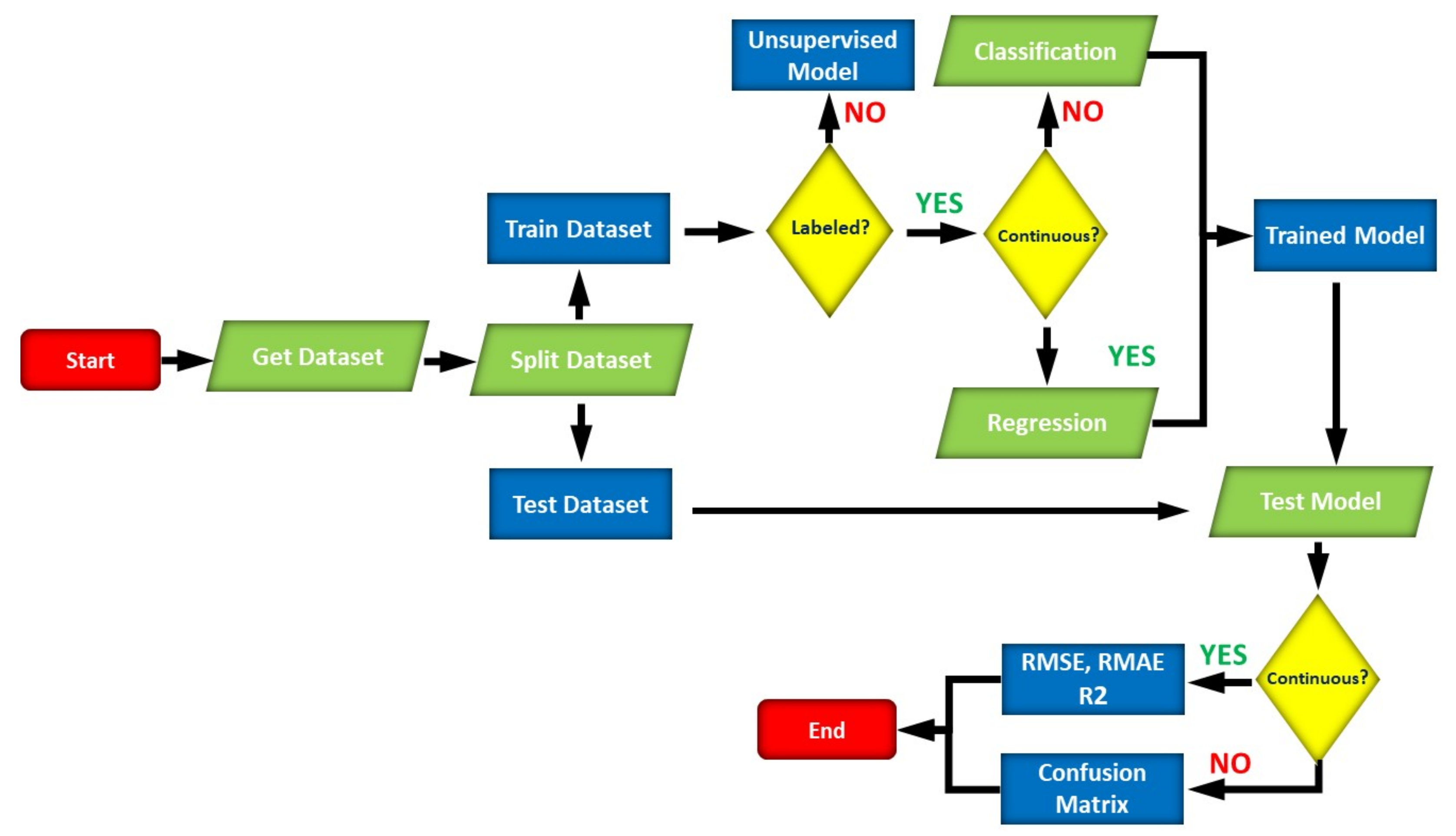
In this research work, we used the generic scientific methodology, following a typical machine-learning approach consisting of the following phases: data gathering, data processing, feature selection, building machine-learning models, and model testing and validation. Figure 1 shows a generic flowchart of how to build a typical machine-learning model. The flowchart starts by gathering raw data to work with. During this step, several preprocessing operations can be applied to translate the raw data into a suitable format acceptable by machine-learning algorithms, such as normalization, standardization, feature scaling, and Principal Component Analysis (PCA).

Next, the dataset is split into two parts: training and testing. Best practices recommend splitting the dataset into 80% for training and 20% for testing, other divisions are also applicable based on the dataset and application domains. Machine-learning algorithms are broadly classified into two categories: supervised and unsupervised learning. Supervised learning works with labeled data, i.e., when the target values are known to the machine-learning models in advance, whereas in unsupervised learning the data is unlabeled; in this case, clustering algorithms can be used to group relevant samples based on some similarity measures.

Supervised learning is further divided into two sets of techniques: classification and regression. When the features contain continuous numeric values, the regression algorithms can be applied, and the classification algorithms are applied for features with categorical data. Next, the machine-learning models will be trained on the training set to build the model. The built model is validated using the testing set to calculate its accuracy, and it can be retrained until a satisfactory accuracy is achieved. In classification problems, the confusion matrix can be used as a performance measure to check the accuracy, whereas several statistical error metrics can be used to analyze the regression models, such as MSE, MAE, and R².

3.2. Machine-Learning Algorithms

Of the number of prediction techniques, machine-learning regression and Deep Neural Networks (DNNs) are two common types of Artificial Intelligence (AI) models, which are extensively used for wind speed prediction [32,33,34]. Support Vector Machine (SVM) is a commonly used model for wind speed prediction [35]. These models can be easily applied to specific wind speed data without considering any local wind variations [36].

Due to the high variation of wind speed, the model accuracy is tied with wind data spatial and temporal dependencies [37]. Multiple Linear Regression (MLR), ridge regression, lasso regression, random forest, SVR, and ANN are the six machine-learning methods experimented in this work [38,39]. These models were selected in this study because regression models, CNN, and Long Short-Term Memory (LSTM) showed the best accuracy under different weather types [40]. A brief description of each algorithm used in this research is given below.

3.2.1. Multiple Linear Regression (MLR)

Machine-learning-based regression techniques, also known as multiple regression, are statistical methods being widely used to study relationships between variables. They correlate multiple independent variables (predictors) to predict the target output (dependent variable). Since MLRs can connect more than one independent variable, they are considered as an extension to the Ordinary Least Squares (OLS) regression. Given a set (n) of independent variables $\{x_1+x_2+x_3+x_4+\dots +x_n\},x_n \in R$, and m a number of samples, the MLR model can be mathematically represented by the following equation (Equation (1)) [21].

$${\widehat{y}}_i={\beta }_0+{\beta }_1{x}_{i1}+{\beta }_2{x}_{i2}+{\beta }_3{x}_{i3}+\cdots +{\beta }_n{x}_{in}+{ϵ}_i , \left(i=1, 2, 3,\dots ,m\right)$$

(1)

where $y_i \in R$ is the dependent variable, ${\widehat{y}}_i$ is the estimation of γ_i, ϵ is the deviation of ${\widehat{y}}_i$ from its mean value; β is the regressor coefficients estimated from least-square estimates, β₀ is the intercept, β_n is the slope of the regression line, and m is the number of data samples.

3.2.2. Ridge Regression

Ridge regression is a variant of MLR, it is mainly used when the dataset suffers from multicollinearity, i.e., when the correlation between independent variables is too high, which makes the least squares estimate producing unbiased results that might be far from the true values. When the regression estimates consider this degree of bias, the ridge regression can reduce the standard errors to minimum levels. The mathematical representation of the ridge regression is similar to the MLR with some constrains as illustrated in Equation (2).

Here, C denotes the number of boundaries of the ridge regression. The regularization shrinks the parameters to reduce the model complexity by a penalty hyperparameter factor (λ), denoted as a coefficient of shrinkage as depicted in Equation (3). The true difference between MLR and ridge regression is that the second part of Equation (2) contains the constraint (B), which is calculated following Equation (4), and multiplied by the penalty factor (λ). The existence of this factor will decrease the residual error, and hence, the ridge regression might achieve higher accuracy [22,41].

$${\beta }_0{}^2 +{\beta }_1{}^2+{\beta }_2{}^2+\cdots +{\beta }_n{}^2\le C^2$$

(2)

$${\widehat{\beta }}^{ridge}=argmin{\sum }_{i=1}^n{\left[y_i-{\widehat{y}}_i\right]}^2=argmin \min ({\left|\left|y_i-XB\right|\right|}_2^2+\lambda {\left|\left|B\right|\right|}_2^2)$$

(3)

$${\left|\left|B\right|\right|}_2=\sqrt{{\beta }_0{}^2+{\beta }_1{}^2+{\beta }_2{}^2+\cdots +{\beta }_n{}^2}$$

(4)

3.2.3. Lasso Regression

Lasso regression is another variant of MLR that is also suitable for models either having higher levels of multicollinearity, or requiring a partial automation or part selection, such as parameter elimination or variable selection. The lasso regression adopts the shrinkage mechanism and, as such, the data values are shrunk towards a central tendency (mean or median) [42], which makes it appropriate for simple or sparse models with few features.

Compared to the ridge regression, the lasso regression tends to make the coefficients approach absolute zero. As depicted in Equation (5), the mathematical model of the lasso regression can be easily extracted from the ridge regression with a minor difference in such a way that the second term of Equation (3), in which the lasso regression adds a level of penalty equals the absolute value of the magnitude of the coefficients, it uses L₁ regularization to force the coefficients approaching zero, and it can be eliminated from the model.

Larger penalties can cause some coefficient values to be as much closer to zero as possible, which is the ideal theme to produce simpler models. Moreover, L₂ regularization (used by the ridge regression) does not result in the elimination of the coefficients or encouraging sparse models. The key difference between L₁ and L₂ is that L₁ is the sum of the weights, while L₂ is the sum of the square of the weights.

$${\widehat{\beta }}^{lasso}=argmin{\displaystyle \sum }_{i=1}^n{\left[y_i-{\widehat{y}}_i\right]}^2=argmin \min ({\left|\left|y_i-XB\right|\right|}_2^2+\lambda {||\beta ||}_1$$

(5)

3.2.4. Random Forest

Random forest is a common machine-learning algorithm utilizing the principle of ensemble learning; it is a technique that combines multiple classifiers/decision trees to make a more accurate prediction. Each decision tree makes the prediction based on its own training process applied on a randomly selected subset of the data. The random forest is trained through a technique called bootstrap aggregation; commonly known as bagging that requires training each tree on random samples, where sampling is done with replacement to provide a better knowledge of the bias and the variance. As the number of trees increases, the precision of the output does as well [43].

3.2.5. Support Vector Regression (SVR)

The Support Vector Machine (SVM) uses a principle called structural risk minimization inductive to provide a satisfactory generalization on a limited dataset. It can fit very well for both regression and classification problems. The SVR is an instance of SVM that mainly deals with regression problems aiming at fitting the error within a fixed value, which is mainly associated with problems in the process of selecting the right decision boundary.

The best fit is achieved when the number of data points between the boundaries reaches its maximum value. The SVM can handle a variety of transfer functions, such as linear, non-linear, polynomial, and radial basis functions. For a simple linear regression case, given a set of predictors (x_i) and a response (${\widehat{y}}_i$), the SVR model is mathematically represented following Equation (6), where f_i (x) describes the kernel or the transfer function, and b is a constant value representing the model’s bias [44].

$${\widehat{y}}_i={\displaystyle \sum }_{i=1}^n{\beta }_i{f}_i\left(x\right)+b$$

(6)

3.2.6. RNN-LSTM

An ANN is a collection of connected nodes called artificial neurons distributed among three levels of layers: an input layer, one/more hidden layers, and an output layer, where neutrons of one layer are linked to the neurons of a previous layer. The Convolutional Neural network (CNN) and the Recurrent Neural Network (RNN) are two common types of ANN. The CNN (ConvNet) approach uses a mathematical convolution rather than a matrix multiplication to build the prediction model, and it is capable of modeling complex nonlinear relationships between input and output layers through training and learning processes.

This model has the capability to self-learn, self-organize, and self-adapt without requiring explicit mathematical expressions compared to the physical approach [45]. Each artificial neuron receives input signals (x₁, x₂, … x_m), multiplies each input by a weight (w₁, w₂, … w_m), adds them together with a predetermined bias, and passes them through the activation function, f(x). The signal produces an output of either 0 or 1 based on the activation function threshold’s value. A perceptron with its set of inputs, set of weights, its summation and bias, its activation function, and the target output all together forms a single layer perceptron.

In a practical implementation of the ANN, some hidden layers are added between the input and output layers, and this number is a hyperparameter—it is determined by trial and error to achieve the intended model accuracy. In this research, RNN-LSTM was implemented due to its highest prediction accuracy. Essentially, the learning process of the LSTM can create self-loops to produce common paths in which the gradient can arise for a long-time period. The LSTM is explicitly designed to circumvent long-term dependency problems, and it can be mathematically represented by the following set of equations: Equations (7)–(11) [41].

$$f\left(t\right)={\sigma }_g\left(W_f{x}_t+U_f{h}_{t-1}+b_f\right)$$

(7)

$$i_t={\sigma }_g\left(W_i{x}_t+U_i{h}_{t-1}+b_i\right)$$

(8)

$$o_t={\sigma }_g\left(W_o{x}_t+U_o{h}_{t-1}+b_o\right)$$

(9)

$$c_t=f_t \circ c_{t-1}+i_t \circ {\sigma }_c\left(W_c{x}_t+U_c{h}_{t-1}+b_c\right)$$

(10)

$$h_t=o_t \circ {\sigma }_h\left(c_t\right)$$

(11)

where $x_t\in R^d$ is the input vector to the LSTM unit, $f_t\in R^h$ is the forget states activation vector, $i_t\in R^h$ is the input or update gate’s activation vector, $o_t\in R^h$ is the output gate’s activation vector, $h_t\in R^h$ is the hidden state vector, $c_t\in R^h$ is the cell state vector, $W\in R^{hxd}, U\in R^{hxh}, \mathrm{and} b\in R^h$ are weight matrices and bias parameters, which are must be learnt during the training phase, ${\sigma }_g$ is the Sigmoid function, and ${\sigma }_c$ is the hyperbolic tangent function.

3.3. Evaluation Metrics

Several common evaluation metrics were used to test and compare the performance of the six machine-learning algorithms and to find the optimal model that accurately represents the data and produces a higher prediction accuracy for unseen data. Therefore, following an accurate evaluation procedure is considered an integral part of the model development process, since some of the evaluation procedures might produce over-optimistic and overfitted models [46,47].

Two methods are commonly used to evaluate prediction models applied to datasets: cross-validation and hold out [48,49]. During model training, the cross-validation method is used to choose the best models having the highest accuracy among others. To avoid overfitting, the models were applied again on the test dataset (20%) using the hold out method to evaluate models’ performance on unseen data [50]. During the testing step, various evaluation measures can be used to compare the performance of the considered models.

There is a wealth of criteria by which the models were evaluated and compared. The evaluation procedures used in this work are four performance indicators determined by Equations (12)–(15). Mean Absolute Error (MAE), Mean Square Error (MSE), Mean Absolute Deviation (MAD), and coefficient of determination (R²) [51]. MAE uses the same unit as the original data, and the models can be compared using this metric when errors are measured in the same units.

The MSE provides the amount of error in the statistical models. It measures the average squared differences between observed and estimated values. In optimal scenarios (accuracy = 100%), the MSE will be zero. The MAD is the average distance between each data point and the mean, it measures the variability in a dataset. R² determines the amount of variance of the dependent variables described by the prediction model, and an optimal prediction model has the value of R² very close to 1.

It is worth mentioning that any one of the aforementioned statistical procedures can be used to give precise performance analyses that help in ranking the prediction models.

$$MAE={\displaystyle \sum }_{i=1}^n\frac{\left|{\widehat{v}}_i-v_i\right|}{n}$$

(12)

$$MSE={\displaystyle \sum }_{i=1}^n\frac{{\left({\widehat{v}}_i-v_i\right)}^2}{n}$$

(13)

$$MAD={\displaystyle \sum }_{i=1}^n\frac{\left|v_i-\overline{v}\right|}{n}$$

(14)

$$R^2=1-\frac{{{\displaystyle \sum }}_{i=1}^n {\left(v_i-{\widehat{v}}_i\right)}^2}{{{\displaystyle \sum }}_{i=1}^n {\left(v_i-\overline{v}\right)}^2}$$

(15)

where ${\widehat{v}}_i$ is the predicted speed value, $v_i$ is the actual wind value,$\overline{v}$ is the average wind speed value, and n is the number of wind speed samples.

4. Dataset Exploration and Processing

This research work was done in West Bank—Palestine; located on the Eastern coast of the Mediterranean Sea with altitude ranging from (−276–1000 m) above the sea level. In this region, the climate conditions change frequently with cold and rainy periods in winter, and mild and hot periods in summer with relative humidity ranges between (51–83%). As with other developing countries, the energy demands of the Palestinian people have increased in recent years. Residents of this region require a great deal of energy to achieve their sustainable development. Nevertheless, several challenges prevent accomplishing this sustainability. Some of these challenges are due to economic, political, environmental, and social issues.

The wind data profile used to train, test, and validate the machine-learning algorithms were taken from the Palestinian meteorological stations’ network in the period from 1 January 2008 to 31 December 2018 (11 years). The gathered wind data were continuously logged at a height of 20 m using a cup generator anemometer located at Jabal Al-Mukabber’s village in East Jerusalem.

Table 1. Geographical coordinates of the metrological station in East Jerusalem.

Variable	Value
Latitude	31.7555° N
Longitude	35.2410° E
Anemometer height	20 m above ground level
Elevation	720 m above sea level

shows the coordinates of the metrological station of the study site. The dataset contained five variables: timestamp, wind direction, wind speed, air temperature, and atmospheric pressure. The readings are measured at a frequency of 3 h (8 measurements for each day).

During the analysis of the data matrix as presented in

Table 2. Wind speed data analysis based on minimum, mean, max, SD, 25th, 50th, and 75th percentiles of the wind speed dataset.

	Temp (°C)	Pressure (mbar)	Direction (Degrees)	Speed (m/s)
Mean	18.22	922.55	233.97	3.11
SD	6.98	3.67	91.5	1.54
Min	0	909.0	0	0
25%	12.6	919.9	170.0	2.0
50%	18.5	922.3	270.0	3.0
75%	23.4	924.9	300.0	4.0
Max	39.7	937.3	360.0	14.5

, we found that each variable had 32,131 records. The mean wind speed was found to be 3.11 m/s with a standard deviation of 1.54 m/s, 120 records having null values in the wind speed variable, and the registered maximum wind speed value was 14.5 m/s. The measured air temperature values ranged from 0 to 39.7 °C with a mean value of 18.22 °C, while the measured values of the atmospheric pressure ranged from (909–939.3 mbar).

The wind direction was registered in the form of 0 to 360 degrees, according to the mean of the wind direction, and the overall direction of the wind was found to be southwest. The dataset was provided in xlsx file having 11 sheets (one for each year).

Before applying the models, we performed some data preprocessing functions to remove null values and applied some normalization techniques that are required by some machine-learning algorithms considered in this study. As shown in the literature, and as a common best practice, the dataset was randomly split into two parts: a training set that constitutes (80%) and a testing set that constitutes (20%) of the whole data. Table 2 shows the distribution of the wind speed data showing the minimum, median, and maximum quartiles.

It shows the complete wind speed data distribution among the whole period (11 years). 75% of the temperature values are less than 23.4 °C, which represents a moderate temperature in the study area. Moreover, 75% of the wind speed dataset is less than or equal to 4 m/s, which is a moderate value, and it is suitable for small turbines, 75% of the atmospheric pressure values are below 925 mbar, 25% of wind direction was found to be northwest, 50% to the south, and 75% to the southeast direction.

Figure 2 shows the full timeline of the dataset. For each variable, it shows its possible values distributed among the whole period. The correlation table and correlation matrix of the dataset experimented in this study are presented in

Table 3. Correlation matrix that shows the correlation coefficients between dataset variables.

	Time	Temperature	Pressure	Direction	Speed
Time	1.000	0.036	0.031	0.046	−0.084
Temperature	0.036	1.000	−0.414	0.166	0.012
Pressure	0.031	−0.414	1.000	−0.324	−0.346
Direction	0.046	0.166	−0.324	1.000	0.349
Speed	−0.084	0.012	−0.346	0.349	1.000

and Figure 3, respectively. They used to indicate the direction and degree of the relationship between the variables in the dataset where the statistical analysis was conducted. The relationship could be a positive (+) or a negative (−) value corresponding to a correlation between any two variables. According to Figure 3, it is determined that the pressure variable has a moderate negative relationship with the wind speed and a medium positive correlation with the direction. The pairplots of all variables are shown in Figure 4.

5. Experimental Results and Discussion

Multiple machine-learning algorithms were applied on the dataset to predict wind speed, which includes multiple linear regression, lasso regression, ridge regression, support vector regression, random forest, and Long Short-term Memory (LSTM). The simulation testbed used Intel(R) Core(TM) i7-8565U CPU running @ 1.80 GHz, 1.99 GHz with 16 GB memory, 64 bit MS Windows 10 Pro with x64 processor architecture, The Python environment setup consisted of Anaconda (4.10.3) with Python (3.8.11) and common ML libraries, mainly scikit-learn (0.24.2) and keras (2.7.0), among other libraries for data extraction and visualization, such as seaborn and matplotlib. The dataset was split into training and testing sets, 80% (28,017) and 20% (3214) from 2008 to 2018, respectively. The models are trained using the training dataset, and the performance results are presented in

Table 4. Statistical error measures for machine-learning algorithms of the test dataset.

ML Algorithm	MAE (m/s)	MSE (m/s)	MAD (m/s)	R2 Score
MLR	1.068	1.88	0.883	0.21
Ridge (alpha = 100)	1.067	1.897	0.885	0.203
Lasso (alpha = 0.0001)	1.068	1.881	0.882	0.21
Random Forest (n = 200)	0.894	1.345	0.715	0.435
SVR (Linear)	1.066	1.916	0.884	0.195
LSTM	0.938	1.471	0.762	0.382

.

For the ridge regression, several experiments were conducted to choose the best value of alpha. Of the various tested values (0.1, 1.0, 10, 100, and 1000), alpha = 100 was chosen. Similarly, for the lasso regression, from the values 0.1, 0.01, 0.001, and 0.0001, alpha = 0.0001 was chosen as it gives the best accuracy of the model. For the SVR, the kernel initializer was set to linear, and the default settings for the other parameters were used. The number of trees (n) in the random forest was set to 200 after several trials and errors, and other parameters remained in their default states. On the other hand, the activation function of the LSTM was set to linear, and it consisted of 50 hidden layers, the model was sequential, the number of train epochs was 500, and the batch size was fixed to 1.

Figure 5 shows the prediction visualization of the six algorithms. For each algorithm, its subplot shows the predicated vs. actual wind speed values. By referring to these subplots, a clear pattern was found in the prediction visualization for the random forest followed by the LSTM, which verifies the accuracy measures listed in Table 4, while the rest of the other regressions show large outliers.

The MAE, MSE, and MAD provided lower values for the random forest and the LSTM models compared to the other methods, the combination of the statistical performance results showed that the SVR is the worst prediction model for wind speed with R² = 0.195, while R² for the random forest and the LSTM models are found to be 0.435 and 0.382, respectively. According to the MAE values, slightly larger residual errors were found for the LSTM model than the random forest model. Overall, the random forest and the LSTM-RNN models are denser, while the other models provide a disperse prediction.

Figure 6 illustrates the LSTM model loss (top) and the statistical error measures per epoch (bottom), the model was run for 500 epochs. By observing the graphs, the loss, MAE, and MSE show a descendant trend, which indicates that the model can provide better prediction accuracy with higher reliability for future wind speed prediction.

In summary, wind speed is directly related to various weather conditions, bearing in mind that the fickle nature of the weather and the greater degree of wind uncertainty make wind prediction a big challenge. A viable solution is to run multiple machine-learning models in parallel to short, medium, and long-term wind speed predictions to obtain the maximum strategic and operational decisions of the energy production from wind profiles.

6. Conclusions and Future Work

An effective wind speed prediction plays an important role in developing highly utilized wind energy projects. Multiple prediction techniques have been applied to wind speed data with promising results worldwide. However, the accuracy of prediction techniques is highly dependent on the considered metrological station and the wind profiles; this means that the optimal prediction model for one site might not be the optimal for other sites. In this research study, we investigated multiple artificial intelligence algorithms to predict wind speed in East Jerusalem meteorological station (31.7555° N, 35.2410° E) over the period 2008–2018. The wind speed prediction has been estimated using six machine-learning algorithms, namely multiple linear regression, ridge, lasso, random forest, support vector, and the LSTM.

Therefore, timestamp, direction, pressure, and temperature were introduced to the machine-learning algorithms to realize the estimation. The relationships among variables were determined using the correlation matrix and it is found that pressure is highly negatively correlated with wind speed. According to the carried out estimation processes, the random forest method followed by the LSTM are determined as successful estimators of wind speed prediction with the lowest error metric scores compared to the other methods. As a future work, we will investigate other wind speed profiles and metrological station characteristics collected from other sites to develop more powerful prediction models, as well as apply mixed machine-learning algorithms to obtain better accuracy.