Short-Term Load Forecasting Model of Electric Vehicle Charging Load Based on MCCNN-TCN

Abstract

The large fluctuations in charging loads of electric vehicles (EVs) make short-term forecasting challenging. In order to improve the short-term load forecasting performance of EV charging load, a corresponding model-based multi-channel convolutional neural network and temporal convolutional network (MCCNN-TCN) are proposed. The multi-channel convolutional neural network (MCCNN) can extract the fluctuation characteristics of EV charging load at various time scales, while the temporal convolutional network (TCN) can build a time-series dependence between the fluctuation characteristics and the forecasted load. In addition, an additional BP network maps the selected meteorological and date features into a high-dimensional feature vector, which is spliced with the output of the TCN. According to experimental results employing urban charging station load data from a city in northern China, the proposed model is more accurate than artificial neural network (ANN), long short-term memory (LSTM), convolutional neural networks and long short-term memory (CNN-LSTM), and TCN models. The MCCNN-TCN model outperforms the ANN, LSTM, CNN-LSTM, and TCN by 14.09%, 25.13%, 27.32%, and 4.48%, respectively, in terms of the mean absolute percentage error.

1. Introduction

The growth of the electric vehicle industry has captivated governments, automakers, and energy companies. EVs are seen as a viable solution to the depletion of fossil resources and rising pollution [1]. It is widely believed that the popularity of EVs can reduce greenhouse gas emissions (mainly carbon dioxide) [2]. Meanwhile, falling battery prices and government incentives will also promote rapid growth in the scale of EVs [3]. However, the increased charging demand resulting from the rapid development of EVs also poses various challenges to the grid. The EV charging load has a great impact on the stable operation of the distribution network [4], including the decline of power quality and the difficulty of optimizing and controlling the operation of the power grid [5,6]. The research on EV charging load forecasting is carried out not only to ensure the economical and stable operation of the power system [7] but also to support the development of EVs [8].

EV charging load forecasting approaches are now separated into probabilistic models, time series models, and machine learning models. The probabilistic modeling method establishes probabilistic models of residents’ charging and travel behavior using statistical and queuing theory, followed by load forecasts using Monte Carlo simulation. Taylor J et al. [9] utilized the Monte Carlo method to establish a large-scale charging demand model, considering EV type, penetration rate, charging scenario, etc. In [10], it is assumed that the arrival time of EVs at the charging station follows Poisson distribution, and the charging load prediction is carried out based on queuing theory. With the deepening of research, the temporal and spatial distribution of EV charging load has attracted the interest of many researchers. Shun et al. [11] established a probabilistic model of the temporal and spatial distribution of EVs based on travel chains and Markov decision processes. Chen et al. [12] applied the OD matrix analysis method to plan the driving path of the logistics electric vehicle and solve the charging demand load value through the mixed-integer programming model. Xing et al. [13] proposed a data-driven EV charging load prediction method, which is based on Didi user travel data to establish a traffic network model, a vehicle spatiotemporal transfer model, and a resident travel probability model.

Currently, time series and machine learning algorithms are commonly employed to forecast EV charging load in the short term. The exponential smoothing model [14], the linear regression (LR) model [15], and the autoregressive integrated moving average (ARIMA) model [16] are the most often used time series models. While time series models have straightforward structures and require minimal training, they are incapable of capturing the nonlinear properties of load series. With the rapid advancement of artificial intelligence technology, intelligent algorithms such as artificial neural networks (ANNs) and deep neural networks are increasingly used to forecast EV charging load. The neural network has excellent power for feature extraction and the ability to form nonlinear mapping relationships [17], which effectively addresses the time series model’s shortcomings. In [18], the SVR founded on an evolutionary algorithm is proposed for electric bus charging load forecasting. Yi et al. [19] proposed a multi-step EV load prediction model established on long short-term memory (LSTM), and the results suggest that the model is capable of accurately predicting sequence data. In [20], LSTM models show better performance and provide higher accuracy compared to the prediction results of ANNs. The gated recurrent unit (GRU) is a characteristic and efficient variant of LSTM. The GRU is characterized by making the network structure simpler. Zhu et al. [21] introduced GRU into short-term forecasting of EV charging load. In order to further improve the short-term load forecasting performance, some forecasting methods combined with LSTM and other recurrent neural networks (RNN) have also been proposed. Feng et al. [22] proposed an EV charging load prediction method based on a combination of the multivariate residual corrected grey model (EMGM) and LSTM network. Dabbaghjamanesh et al. [23] applied Q-Learning Technique based on ANN and RNN to improve the short-term prediction accuracy of EV charging load. The model based on LSTM and GRU is capable of learning long-term temporal correlations; however, due to the lack of convolution in the model, the feature extraction capability still has to be enhanced. Therefore, it is difficult for the above models to effectively utilize and extract the feature information in the EV charging load.

When confronted with this problem, approaches for extracting features are seen to be one of the most viable solutions. The convolutional neural networks (CNN) have excellent feature extraction [24], which is often used for feature extraction in short-term load forecasting. Li et al. [25] applied an evolutionary algorithm-optimized CNN model for EV charging load prediction. In addition, the CNN-LSTM model combining CNN and LSTM is often used in traditional short-term forecasting of power loads [26]. In the CNN-LSTM model, CNN extracts the feature information of load-related influencing factors, and LSTM is used to learn the temporal dependency between the feature information sequence extracted by CNN and the output [27]. Yan et al. [28] proposed a hybrid model based on CNN and LSTM to predict the short-term electricity load of a single household. However, most methods ignore the long-term temporal relationship of input variables, causing the load forecasting model to lack adequate prior knowledge.

Furthermore, EVs are abundant in urban areas, and EV users’ travel behavior is influenced by many random factors, resulting in increasingly complicated fluctuations in the charging load of EVs. Given this problem, accurate forecasting by using a short-term load forecasting model on a single time scale is difficult [29]. Short-term load forecasting can be enhanced by decomposing the load into multiple intrinsic mode functions and then separately predicting and reconstructing the sub-model prediction results [30]. Wang et al. [31] proposed a “decomposition-predict-reconstruction” prediction model based on empirical mode decomposition (EMD) and LSTM, which effectively improved the accuracy of load prediction.

One-dimensional convolutional neural networks (1DCNN) can extract one-dimensional sequence features, commonly used to extract time series feature information. Wang et al. [32] utilized 1DCNN to extract the fusion features of bearing vibration signal and sound signal to realize bearing fault diagnosis. In [33], the influent load is first decomposed by EMD, and then 1DCNN extracts the latent features of each intrinsic mode function’s periodic signal. However, although the 1DCNN model can achieve feature extraction at various time scales by adjusting the scope of the receptive field, it cannot extract the time series dependencies between time series data. With the advent of advanced TCN models that combine the advantages of CNN feature processing and RNN time-domain modeling, it is possible to extract time series dependencies between long intervals of historical data [34]. Yin et al. [35] proposed a feature fusion TCN structure that fuses model output features at multiple time delay scales. The TCN built on the convolutional network can process data in parallel on a large scale and has a faster computing speed than the RNN such as LSTM [36]. Although the signal decomposition method can obtain the components of EV charging load at various time scales, it still necessitates the selection and construction of low-dimensional features with a high degree of differentiation, which not only adds subjectivity and complexity to this identification method but also risks losing important information.

On the basis of the foregoing research, an EV charging load forecasting model based on the MCCNN-TCN is proposed in this paper. The MCCNN model can mine the fluctuation features of EV charging load at multi-time scales. The TCN model can establish the global time-series dependencies between the local time-series feature information at different time scales extracted by the MCCNN model. In addition, accurate load forecasting is frequently reliant on a thorough understanding of the elements that contribute to increasing or decreasing consumer demand [37]. The EV charging load is affected by numerous aspects, including weather temperature, date type, traffic conditions, user travel behavior, etc. [8]. Therefore, this paper introduces the maximum information coefficient (MIC) and Spearman rank correlation coefficient and proposes a similar day method based on weighted gray correlation analysis to screen historical loads. The main contributions of this paper are described as follows:

(1)

The MIC was applied to eliminate input data redundancy and reduce the complexity of the model. The MIC was used to choose meteorological variables that have a substantial link with EV charging load. The selected meteorological variables were utilized as an input to both the prediction and comparable day selection models;

(2)

A similar day selection model based on weighted grey relational analysis was proposed. The Spearman rank correlation coefficient of the week average daily load was used to calculate week type similarity. Then, by selecting meteorological variables obtained by MIC and week type similarity as the input, a similar day selection model based on weighted gray correlation analysis was used to choose a similar day load used as the forecasting model’s input;

(3)

An MCCNN-TCN model framework was built. Combining the multi-channel 1DCNN model with the TCN model can establish global temporal dependencies between time series features at multiple time scales, which effectively improves the prediction performance.

The remainder of this paper is organized as follows. In Section 2, a short-term EV charging load forecasting framework based on the MCCNN-TCN model is introduced. In Section 3, experiments are conducted with a real dataset of grid companies and compared with other models. In Section 4, the model proposed in this paper is analyzed compared to other state-of-the-art methods based on experimental results. In Section 5, the paper’s conclusions and future research are given.

2. Materials and Methods

2.1. Selecting Similar Days

2.1.1. Screening of Meteorological Features Based on Maximum Information Coefficient

As a new type of electric load, EV charging load is not only related to residents’ travel behavior but also affected by meteorological factors such as weather and temperature [38]. In order to lower the input size of the similar day model and forecast model, relevant meteorological features that strongly correlate with EV charging load must be selected [36]. At the same time, since meteorological features and EV charging load are both nonlinear time series, this paper uses MIC to examine the nonlinear relationship between each meteorological variable and EV charging load. Unlike other traditional correlation analysis methods, the benefit of MIC is that it does not require any assumptions about the data distribution and is acceptable for both linear and nonlinear data [39]. The MIC is calculated as follows [40].

For a binary dataset, D and $D\in R^2$, divide D into a grid of x rows and y columns. The obtained grid G based on different division methods forms set A. Find the maximum mutual information $\max I\left(D|G\right)$ in set A, conserve it as:

$$I^{*}(D,x,y)=\underset{G\in A}{\max }I(D|G)$$

(1)

where $D|G$ is the distribution of the binary data set D on the grid G.

The maximum normalized mutual information of the binary dataset D at different scales is formed into the feature matrix $M\left(D\right)$, and the elements of the feature matrix are defined as:

$$M{(D)}_{x,y}=\frac{I^{*}(D,x,y)}{{\log }_2\min (x,y)}$$

(2)

The MIC is calculated by:

$$MIC(D)=\underset{rc<B(n)}{\max }\{M{(D)}_{x,y}\}$$

(3)

where n indicates the size of the sample, $B\left(n\right)$ is a function about the size of the sample, and the constraint indicating the total number rc of squares of the grid G is less than $B\left(n\right)$, generally $B\left(n\right)=n^{0.6}$ [41]. A greater MIC value between the two variables indicates a stronger correlation.

2.1.2. Quantifying Week Type Similarity Based on Spearman Correlation Analysis

The characteristics of EV charging load in different months, seasons, and week kinds are investigated in this article to study the relationship between EV charging load and date types. The EV charging load has the maximum consumption level in December and the lowest in April, as shown in Figure A1 in the Appendix A. The consumption level of EV charging load in winter and fall is significantly higher than in spring and summer, and the load in winter represents a tendency of rising first and then reduce. In contrast, the load in summer has a fluctuating and rising trend, as shown in Figure A2 in the Appendix A. EV charging load consumption level is highest on Saturday and lowest on Monday, as shown in Appendix A Figure A3. In summary, it is critical to pay attention to the effect of date type on the charging load of EVs. In this paper, the date types were divided into season types and week types, and the similarity between week types under each season was established as the input of the similar day model. In order to avoid human subjective participation in setting the week types map value, using the average daily EV charging load between week types calculated the similarity between week types in this paper.

The data on electric vehicle charging load do not follow a normal distribution. Additionally, the Spearman coefficient does not require that the data remain normal [42]. As a result, this paper proposes utilizing the Spearman coefficient to quantify the similarity of week types. The week types under each season were divided into seven (Monday to Sunday), and then the Spearman coefficient was calculated for the average daily load between the week types. The correlation value indicative is represented by $F_{kg}^h$, as in (4):

$$F_{kg}^h=1-\frac{6{\displaystyle \sum }{A}_t^2}{n\left(n^2-1\right)} t=1,\dots ,96$$

(4)

where k and g represent the week type; h represents the season, $h=1, 2, 3, 4$; n is the load sample number; and A_t indicates the difference of the position between the t-th daily load samples of week type k and week type g.

2.1.3. Similar Days Selection Model Based on Weighted Grey Correlation Analysis

When calculating the gray correlation, the traditional gray correlation analysis assigns the same weight to each feature, ignoring each influencing factor’s difference [43]. Therefore, each influencing factor’s weight is first analyzed based on the improved entropy weight method in this paper. Then the correlation degree between the forecasting day and history day is calculated based on the weighted grey correlation degree analysis.

According to the historical data, the entropy $E_j$ of the j-th meteorological feature is calculated [44]:

$$\{\begin{array}{c}{E}_j=\alpha ·{\displaystyle {\displaystyle \sum }_n^{i=1}}{b}_{ij}\ln b_{ij}, j=1,2,\cdots ,m\\ \alpha =-\frac{1}{\ln n}\\ b_{ij}=\frac{a_{ij}}{{\displaystyle {\displaystyle \sum }_n^{i=1}}{a}_{ij}}\end{array}$$

(5)

where n is the number of historical days, m indicates the dimension of the day feature; $a_{ij}$ represents the value of the j-th feature of the i-th historical day. Additionally, if $b_{ij}=0$, $b_{ij}\ln b_{ij}=0$.

According to the entropy of each meteorological feature, the weight of the j-th day feature based on the improved entropy weight method is calculated as [45]:

$$w_j=\frac{\exp \left({\displaystyle {\displaystyle \sum }_{t=1}^m}{E}_t+1-E_j\right)-\exp \left(E_j\right)}{{\displaystyle {\displaystyle \sum }_{l=1}^m}\left(\exp \left({\displaystyle {\displaystyle \sum }_{t=1}^m}{E}_t+1-E_l\right)-\exp \left(E_l\right)\right)}$$

(6)

The correlation coefficient of each day’s feature is calculated using gray correlation analysis [18]. The following are the feature sequences of the forecasting and history days:

$$\{\begin{array}{c}{X}_d=\left[x_d\left(1\right),x_d\left(2\right),\cdots ,x_d\left(m\right)\right]\\ X_{d-i}=\left[x_{d-i}\left(1\right),x_{d-i}\left(2\right),\cdots ,x_{d-i}\left(m\right)\right]\end{array}$$

(7)

where $X_d$ represents the feature sequence of the forecasting day d, $X_{d-i}$ represents the factor sequence of the history day d − i. The correlation coefficient of the j-th feature of $X_d$ to $X_{d-i}$ is:

$${\xi }_d^{d-i}(j)=\frac{minmi{n}_k\left|x_d(j)-x_{d-i}(j)\right|+\rho maxma{x}_i\left|x_d(j)-x_{d-i}(j)\right|}{\left|x_d(j)-x_{d-i}(j)\right|+\rho maxma{x}_{ij}\left|x_d(j)-x_{d-i}(j)\right|}$$

(8)

where $x_d(j)$ and $x_{d-i}(j)$ are the j-th feature of the forecasting day d and the history day d − i, respectively, $\rho$ is the distinguishing coefficient and $\rho =0.5$.

Based on calculating the grey correlation coefficients $\xi$ of the factors and their weights $w$, the weighted grey correlation between forecast day d and historical day d − i can be expressed as follows:

$$r_d^{d-i}={\displaystyle \sum _{j=1}^m{w}_j}{\xi }_d^{d-i}\left(j\right)$$

(9)

The first 14 days of the forecasting day are defined as a similar day rough set in this paper. Because the capacity of the similar day rough set is limited, it is not assumed that as the date distance increases, the similarity between the forecasting day and the historical day decreases. Furthermore, derived from the past EV charging load data, the average number of days with a Spearman’s correlation coefficient larger than 0.4 between the forecasting day and each historic day in the similar day rough set is 3. In addition, the adjacent daily load is added to the similar day set to ensure time consistency between the forecasting day load and the historical day load. According to the above analysis, the size of the similar day set in this paper is 4.

2.2. Multi-Channel Convolutional Neural Network and Temporal Convolutional Network Model

Because the charging load of EVs is influenced by various factors, including weather conditions, residents’ travel habits, and the traffic network, there is a high level of short-term volatility, making short-term load forecasting more complex. It was demonstrated that extracting the characteristics of EV charging load at various time scales is an effective strategy for improving prediction accuracy [31]. Different influencing factors affect the features of EV charging load at different time scales. In this regard, the paper proposes the MCCNN-TCN model framework. As illustrated in Figure 1, the model framework is divided into three layers: a multi-channel 1DCNN feature extraction layer, a multi-channel TCN layer, and an output layer. The model framework can extract EV charging load characteristics at various time scales and construct a worldwide time-series dependency between the historical and predicted day loads. The multi-channel 1DCNN is utilized as the gate of the MCCNN-TCN model to extract the local features of the input time series at different time scales. Deepening the TCN network can expand its receptive field, establishing the temporal dependencies between global features. The output layer’s job is to create a nonlinear relationship between the forecasting load, meteorological and calendar features, and historical load. Section 2.1.1 and Section 2.1.2 show that the meteorological and date factors impact the EV charging load, in addition to the influence of the historical load on the forecasting load. As a result, this paper combines the TCN model’s output historical load feature vector with a high-dimensional feature vector derived from meteorological and date features. Then, it is input into a fully connected neural network. The fully connected neural network’s output is forecasting day load.

The length of the 1DCNN layer’s input feature map is sn, where s is the number of similar days and n is the number of daily load samples. The role of the multi-channel 1DCNN is to extract the features of a one-dimensional time series consisting of EV charging load sequences in similar daily sets at different time scales. The TCN layer takes the output of the multi-channel 1DCNN model as input and captures the global temporal dependencies at different time scales. The BP layer maps the feature composed of the meteorological factors simultaneously as the forecasting day load and the date type of forecasting day to the high-dimensional feature space. The high-dimensional feature vector obtained by integrating the BP model’s output and the TCN model’s output is used as the input of the fully connected layer in the output layer of the MCCNN-TCN.

2.2.1. Multi-Channel 1D Convolutional Network Model

CNN is a great neural network model that uses convolution kernels to extract essential information automatically [46]. Figure 2 shows the basic architecture of the 1DCNN, which can extract latent features in time series using multiple convolution kernels of the same weight. The same convolution kernel obtains a class of related features during the convolution process. Its mathematical model is described as [47]:

$$H_i=f\left(H_{i-1}\otimes W_i+b_i\right)$$

(10)

where $H_i$ indicates the input of layer I; $H_{i-1}$ indicates the output of layer i − 1; $W_i$ and $b_i$ indicate the weight matrix and the corresponding bias vector of the convolution kernel of layer i, respectively; $\otimes$ indicates for convolution operation; and $f$ indicates the activation function.

Following the convolution operations, the pooling layer uses data downsampling to downsample a huge matrix into a small one, reducing the amount of computation and avoiding overfitting. The pooling layer mathematical model is as follows:

$$H_i=down\left(H_{i-1}\right)$$

(11)

where $H_{i-1}$ and $H_i$ indicate the features before and after pooling, respectively, and “down()” indicates the pooling function.

As shown in Figure 3, the multi-channel 1DCNN is made up of numerous parallel 1D convolution blocks. The first convolutional layer of the multi-channel 1DCNN has a varied convolution kernel size. Long-term scale characteristics of EV charging load can be extracted using big convolution kernels. Short-time-scale characteristics of EV charging loads can be extracted using little convolution kernels. Rough features of EV charging load at different time scales are obtained after the first convolutional layer. This paper extracts detailed features by adding numerous convolutional layers with a convolution kernel of three to the initial convolutional layer to fully mine the detailed information under various EV charging load time scales. The first convolutional layer kernel size K of each channel is represented as follows:

$$K=2^n+1$$

(12)

where $n\in ( 1,2,3,\dots ,N)$, N is the number of channels. The value of N depends on the length of the input layer time series.

Furthermore, earlier research has revealed that when the depth of the neural network increases, residual connections can effectively handle the problems of gradient disappearance and network overfitting [48]. As a result, each channel of the multi-channel 1DCNN is assigned a residual connection in this paper. The residual connection mathematical model is:

$$x_{l+1}=x_l+F\left(x_l,w_l\right)$$

(13)

where x_l+1 is the output of layer l + 1, x_l is the input of layer l, and $F\left(x_l,w_l\right)$ is the residual of layer l.

2.2.2. Temporal Convolutional Network Model

The TCN developed by Bai et al. in 2018 is an algorithm for processing time series [49]. The TCN combines causal convolution, dilated convolution, and residual block to address the problem of extracting long-term time-series information.

The core of TCN is the residual dilated causal convolution unit (RDCCU), which consists of two rounds of dilated causal convolution with the same dilation factor, WeightNorm layer, activation function, Dropout layer, and residual connections formed by direct mapping of the input [35]. Multiple residual dilated causal convolutional units are connected to form a multi-layer TCN network structure, as shown in Figure 4.

The fundamental core structure of the RDCCU is the dilated causal convolution [50], which is composed of causal convolution and dilated convolution [51]. The structure of the dilated causal convolution is shown in Figure 5.

Causal convolution refers to obtaining the output of time t through the convolution of elements at time t and earlier in the previous layer. It ensures that there will be no future information leakage, meeting the requirements of power load forecasting. Dilated convolution can expand the receptive field by increasing the dilation factor [52] and capture long enough historical information without increasing the depth of the model [53], which improves the efficiency of model training. Dilated convolution makes the input of the previous layer sampled at intervals, and the dilation factor d of each layer increases exponentially by 2, which can be described as:

$$l={\displaystyle {\displaystyle \sum }_{d=1}^n\left[\left(K-1\right)\cdot 2^d+1\right]}$$

(14)

As illustrated in Figure 5, the kernel size of each dilated causal convolutional layer is 3. The dilation factor d grows from 1 to 4, which raises the effective history of neurons in the output layer from 3 to 15. In addition, to maintain the whole sequence information, each layer’s output is zero-padded to match the number of input sequences. The mathematical model of dilated causal convolution is as follows [49]:

$$y\left(s\right)=\left(x_d^{*}f\right)\left(s\right)={\displaystyle \sum }_{k-1}^{i=0}f\left(i\right)·x_{s-d·i}$$

(15)

where x is the input and y is the output.

Residual connections are a key structure of the RDCCU. The RDCCU is defined as follows [49]:

$$o=artivation(x+F(x))$$

(16)

The output of the multi-channel 1DCNN is arranged in a T*n two-dimensional data structure according to the channel direction and fed into the first RDCCU of the TCN model. The internal procedure of the RDCCU is shown in Figure 6. The width of the convolution kernel of the RDCCU corresponds to the number of input data channels. The number of output channels of this RDCCU is equal to the number of convolution kernels in the RDCCU. The output of the RDCCU is seamed in the channel direction and used as the input to the next RDCCU.

3. Results

The subject of the study in the paper is EV charging load short-term forecasting in the urban area of a city in northern China. The dataset was data collected from 38 public DC charging stations in the city’s urban area, from 1 January 2019 to 31 March 2020. The number of charging stations in residential, commercial, work and leisure areas is 8, 12, 11, and 7. These charging stations have 298 charging poles, each with a maximum charging power of 60 kW. The dataset included the active power of the charging poles, the transaction power, the charging start time and the charging end time, etc. The active power of the charging poles was sampled at 15 min intervals.

Meteorological data, which can be obtained from China Meteorological Data Network, include the temperature, humidity, precipitation, visibility, wind speed, and weather type. Among them, the temperature, humidity, and precipitation need to be interpolated by spline, and the purpose is to obtain the sampling value simultaneously with the load. Other data includes date type, season, etc.

All of the experimental models were run in the Python 3.6 programming environment, implemented under the Pytorch framework. The hardware used for the experiments was a PC with an Intel Core i7-10300H CPU, NVIDIA RTX 2060 GPU, and 32 GB of RAM.

3.1. Input Variables Selection and Processing

According to the investigation of influencing factors on EV charging load, these factors were divided into meteorological factors, date features, and similar daily load in this paper. Next, three types of features are selected and processed.

The MIC between each meteorological factor and EV charging load was calculated except for weather conditions.

Table 1. Correlation coefficient between electric vehicle charging load and meteorological factors.

	Temperature	Humidity	Precipitation	Visibility	Wind Speed
MIC	0.778	0.788	0.461	0.033	0.343
PCC	0.865	−0.881	−0.459	0.042	0.767

shows the MIC and Pearson correlation coefficient between EV charging load and temperature, humidity, precipitation, visibility, and wind direction. As shown in Table 1, the EV charging load has a strong correlation with temperature, humidity, and rainfall but a weak correlation with visibility and wind speed. At the same time, the influence of weather conditions on the charging load of EVs cannot be ignored [25]. The min–max normalization was used to linearly transform the raw temperature, humidity, and rainfall data to $\left[0,1\right]$. The number of index mapping databases is referenced in Ref. [18]. In this paper, the mapping values were set to 0.1, 0.2, and 0.3 for the weather types sunny, cloudy and overcast, respectively, and 0.7, 0.1, and 1.5 for the weather types light rain or snow, rain or snow, and heavy rain or snow, respectively. Therefore, this paper selected weather type, temperature, humidity, and rainfall as the meteorological features that affect the EV charging load. Thus, this paper selected the temperature, humidity, rainfall, and weather conditions among meteorological factors as similar daily selection and prediction models.

Since the month, season, and week type affect the EV charging load fluctuation characteristics, the season, month, day, week type, weekday, and holiday, selected as date features, were used as the input of the prediction model.

Table 2. Date feature factors.

Date Feature	Detailed Description
Season	1~4 represent spring, summer, fall, and winter
Month	1~12 represent January to December
Day	1~31 represents No. 1 to No. 31
Week	1~7 represents Monday to Sunday
Workday	0 represents a workday, 1 represents a weekend
Holiday	0 represents a non-holiday, 1 represents a holiday

depicts the date features.

Similar daily loads were obtained from the similar days model. The min–max normalization was adopted to constrain EV charging load to $\left[0,1\right]$. After that, the forecasted load values were exponentiated to establish a nonlinear relationship between the exponentially mapped forecasted load values and the historical loads. It eliminates the lagging problem when the model takes the last moment of the input sequence as the forecasting load value.

3.2. Performance Evaluation

The paper considered the root mean square error (RMSE), the mean absolute error (MAE), and the mean absolute percentage error (MAPE) while assessing the performance of the forecasting model. These are the statistical metrics defined:

$$\mathrm{RMSE}=\sqrt{\frac{{\displaystyle {\displaystyle \sum }_N^{i=1}}{\left(y_i-y_{fi}\right)}^2}{N}}$$

(17)

$$\mathrm{MAPE}={\displaystyle {\displaystyle \sum }_N^{i=1}}\left|\frac{y_{fi}-y_i}{y_i}\right|\times \frac{100}{N}$$

(18)

$$\mathrm{MAE}=\frac{1}{N}{\displaystyle {\displaystyle \sum }_N^{i=1}}\left|y_{fi}-y_i\right|$$

(19)

where N indicates the number of validation or testing instances. $y_i$ and $y_{fi}$ represents the actual load and forecasted load of the i-th instance, respectively.

Each statistical metric has different advantages and disadvantages. The RMSE evaluates the performance of a predictive model based on the mean absolute error of the deviation between predicted and actual loads. However, it is susceptible to outliers. In comparison to the RMSE, the MAE reflects the mean absolute error between forecasted and actual loads. It is more resilient to outliers than the RMSE but does not show the real degree of prediction bias. The MAPE is a forecast accuracy measure that considers the relative difference between forecasted and actual loads. However, the MAPE does not apply when the actual load is zero. Therefore, it is vital to employ multiple statistical metrics to assess the prediction performance.

3.3. Similar Daily Load Selection Based on Weighted Grey Correlation Analysis

The weather condition, temperature, humidity, rainfall, and week type are selected as daily features for the similar day in this paper. Since weather conditions and week type similarity are coarse-grained features, while temperature, humidity, and rainfall are fine-grained features, it is necessary to select the coarse-grained amounts of temperature, humidity, and rainfall. This paper selected daily maximum temperature, mean temperature, minimum temperature, as well as daily mean humidity and daily average rainfall as coarse-grained characteristics. Therefore, weather conditions, daily maximum temperature, daily average temperature, daily minimum temperature, humidity, rainfall, and week type similarity were selected as daily features. According to the selected day characteristics and the weighted gray correlation degree, a similar day set of the forecasting day was obtained.

Taking the EV charging load forecast on 15 December 2019 as an example, the weather forecast parameters on that day are shown in

Table 3. Forecasting day meteorological and date type parameters.

Forecasting Day	Week Type	Weather Condition	Maximum Temperature/°C	Minimum Temperature/°C	Mean Temperature/°C	Relative Humidity/%	Mean Rainfall/mm
15 December 2019	Sun	cloudy	0.1	−4.5	−2.4	51	0

. Because the selected December belongs to winter, the week type similarity obtained by Spearman correlation analysis in this season is shown in

Table 4. Values of winter day type similarity.

	Mon	Tues	Wed	Thurs	Fri	Sat	Sun
Mon	1
Tues	0.8271	1
Wed	0.8758	0.9082	1
Thurs	0.7951	0.9044	0.9008	1
Fri	0.8270	0.8485	0.7898	0.8670	1
Sat	0.7800	0.8193	0.8665	0.7986	0.7299	1
Sun	0.9113	0.8573	0.8897	0.7934	0.7698	0.7512	1

.

According to the historical meteorological data and week type before the forecast day (1 December 2019 to 14 December 2019), the weighted grey correlation degrees between the forecasting day and the historical days were calculated to obtain a similar day set. The results of a similar day set are shown in

Table 5. Selection results of similar days.

Date	3 December 2019	6 December 2019	10 December 2019	14 December 2019
similarity	0.7219	0.7773	0.8122	0.6711

.

3.4. Validating the Multi-Channel Convolutional Neural Network and Temporal Convolution Network Model

3.4.1. Hyperparameters of the Multi-Channel Convolutional Neural Network and Temporal Convolution Network Model

From the similar day model results, it can be seen that the length of the similar day historical load sequence of the forecasting day is 384. In this paper, the number of channels of the multi-channel 1DCNN model was set to 4 to fully exploit the characteristics of EV charging load at different time scales. In the multi-channel 1DCNN model, the convolution stride in each channel was set to 1, and the activation function Tanh was selected to perform nonlinear mapping on the results after each convolution. The hyperparameters of the multi-channel 1DCNN model are shown in

Table 6. Layer architecture of the multi-channel 1D convolutional neural network-temporal convolution network.

Channel No.	Layer	Input	Output	Kernel	Kernel Number	Padding	Stride	Activation Function
C1	Input	$1\times 384\times 1$	$1\times 384\times 1$	-		-	-	-
	Residual Layer	$1\times 384\times 1$	$1\times 384\times 1$	-	-	-	-	-
	1D Conv1	$1\times 384\times 1$	$1\times 384\times 4$	$1\times 3$	$4$	1	1	Tanh
	1D Conv2	$1\times 384\times 4$	$1\times 384\times 1$	$4\times 3$	$1$	1	1	Tanh
	1D Conv3	$1\times 384\times 1$	$1\times 384\times 1$	$1\times 3$	$1$	1	1	Tanh
	Adding Layer	$1\times 384\times 1$	$1\times 384\times 1$	-	-	-	-	Tanh
C2	Input	$1\times 384\times 1$	$1\times 384\times 1$	-		-	-	-
	Residual Layer	$1\times 384\times 1$	$1\times 384\times 1$	-	-	-	-	-
	1D Conv1	$1\times 384\times 1$	$1\times 384\times 4$	$1\times 5$	$4$	2	1	Tanh
	1D Conv2	$1\times 384\times 4$	$1\times 384\times 1$	$4\times 3$	$1$	1	1	Tanh
	1D Conv3	$1\times 384\times 1$	$1\times 384\times 1$	$1\times 3$	$1$	1	1	Tanh
	Adding Layer	$1\times 384\times 1$	$1\times 384\times 1$	-	-	-	-	Tanh
C3	Input	$1\times 384\times 1$	$1\times 384\times 1$	-		-	-	-
	Residual Layer	$1\times 384\times 1$	$1\times 384\times 1$	-	-	-	-	-
	1D Conv1	$1\times 384\times 1$	$1\times 384\times 4$	$1\times 9$	$4$	4	1	Tanh
	1D Conv2	$1\times 384\times 4$	$1\times 384\times 1$	$4\times 3$	$1$	1	1	Tanh
	1D Conv3	$1\times 384\times 1$	$1\times 384\times 1$	$1\times 3$	$1$	1	1	Tanh
	Adding Layer	$1\times 384\times 1$	$1\times 384\times 1$	-	-	-	-	Tanh
C4	Input	$1\times 384\times 1$	$1\times 384\times 1$	-		-	-	-
	Residual Layer	$1\times 384\times 1$	$1\times 384\times 1$	-	-	-	-	-
	1D Conv1	$1\times 384\times 1$	$1\times 384\times 4$	$1\times 17$	$4$	8	1	Tanh
	1D Conv2	$1\times 384\times 4$	$1\times 384\times 1$	$4\times 3$	$1$	1	1	Tanh
	1D Conv3	$1\times 384\times 1$	$1\times 384\times 1$	$1\times 3$	$1$	1	1	Tanh
	Adding Layer	$1\times 384\times 1$	$1\times 384\times 1$	-	-	-	-	Tanh

. The TCN model hyperparameters are shown in

Table 7. Layer architecture of the temporal convolutional network.

Layer	Input	Output	Kernel	Dilation	Dropout
Residual blocks 1	$384\times 4$	$384\times 4$	$4\times 3\times 4$	1	0.1
Residual blocks 2	$384\times 4$	$384\times 2$	$4\times 3\times 2$	2	0.1
Residual blocks 3	$384\times 2$	$384\times 1$	$2\times 3\times 1$	4	0.1

. The hyperparameters of the BP model and output layer are shown in

Table 8. Layer architecture of BP and Output layer.

Layer	Input	Output	Activation Function
BP	$10$	$16$	Sigmoid
Output layer	$400$	$1$	-

. In this paper, meteorological features, date features, and similar daily loads were selected as input variables for the MCCNN-TCN model, as shown in

Table 9. Input variables description.

Type of Feature	Variables x	Detailed Description
Load features	x1~x384	Historical load values on the 4 historical similar days
Meteorological features	x385~x388	Temperature, humidity, precipitation at the forecast time t and weather condition on the forecasting day
Date features	x389~x394	Season, month, day, week, workday, holiday on the forecast day

.

3.4.2. Comparative Analysis of Single-Channel and Multi-Channel Convolutional Neural Network and Temporal Convolution Network Model

On the same data set, compared with the prediction results of the single-channel 1DCNN-TCN model, the advanced nature of the MCCNN-TCN proposed in this paper was verified. Each single-channel 1DCNN-TCN and MCCNN-TCN had the same TCN structure, with the only distinction being the number of 1DCNN channels. The single-channel 1DCNN-TCN models were set as follows: Model 1: C1-TCN; Model 2: C2-TCN; Model 3: C3-TCN; Model 4: C4-TCN. Each single-channel 1DCNN-TCN model and MCCNN-TCN model, whose loss function is the MSE, were trained with the Adam optimizer, a learning rate of 0.001, and a batch size of 512.

From 1 June 2019 to 31 August 2019, the training set, validation set, and test set were selected according to the ratio of 8:1:1. Each model outputs a load forecast value at one time each time, and the one-day forecast value refers to the cyclic forecast load value at 96 times. The RMSE, MAPE, and MAE values of each single-channel 1DCNN-TCN and MCCNN-TCN model on the test set are shown in

Table 10. Prediction results of single-channel and multi-channel 1D convolutional neural network and temporal convolution network model.

Layer	RMSE/kW	MAE/kW	MAPE/%
C1-TCN	8.39	6.52	13.42
C2-TCN	9.26	7.32	15.57
C3-TCN	9.68	7.40	15.73
C4-TCN	9.75	7.49	15.88
MCCNN-TCN	7.62	5.79	11.50

.

From Table 10, it can be seen that the prediction performance of Model 1 to Model 4 decreases as the extracted time scale increases. This is due to the fact that the single-channel 1DCNN-TCN at the long-term scale loses the local short-term variation features of the EV charging load. The reason why the prediction performance of Model 1 is lower than that of the MCCNN-TCN model is that Model 1 lacks attention to the change trend features of EV charging load at a long-time scale. The advantage of the MCCNN-TCN model is that it can extract the local short-term change features and long-term change trend features of the EV charging load. Therefore, the RMSE, MAPE, and MAE values of the MCCNN-TCN model are lower than those of the single-channel 1DCNN-TCN models. It can be shown that extracting the multi-scale features of EV charging load can significantly improve the prediction accuracy.

3.4.3. Comparative Analysis of Different Forecasting Models

In order to evaluate the forecasting accuracy and superiority of the model proposed in this paper, ANN, LSTM, CNN-LSTM, and TCN prediction models, whose model structures are shown in Appendix B Figure A4, Figure A5, Figure A6 and Figure A7, were chosen for comparison.

Table 11. Input variables description of ANN, LSTM, and CNN-LSTM models.

Type of Feature	Variable x	Detailed Description
Electrical features	x1~x64	Historical load values from time t to t + 16 on historical similar days
	x65~x80	Historical load values at the time t − 16 to t − 1 on the forecasting day
Meteorological features	x81~x84	Temperature, humidity, precipitation at the forecast time t and weather conditions on the forecasting day
Date features	x85~x90	Season, month, day, week, workday, holiday on the forecast day

shows the ANN, LSTM, and CNN-LSTM models’ input. The TCN model’s inputs are equal to those of the MCCNN-TCN model. The loss function of ANN, LSTM, CNN-LSTM, and TCN models is MSE. Meanwhile, ANN, LSTM, CNN-LSTM, and TCN models were trained with the Adam optimizer, with a learning rate of 0.001 and a batch size of 512. The dataset was selected between 1 January 2019 and 31 March 2020, with an 8:1:1 ratio for the training, validation, and test sets.

The forecasting load curve of the model mentioned above on the test set from 1 March to 7 March 2020 is shown in Figure 7. It can be seen from Figure 7 that the original load is an approximately constant value from 0:00 to 6:00 am every day. The forecasting value of this period, except for the BP model, the forecasting value of all models fluctuates and deviates from the actual value. Although the forecasting value of the ANN model remains constant, it deviates significantly from the actual value. The MCCNN-TCN model fluctuates less than other models and is proximate to the actual value. At the peak of the load curve, the predicted values of the LSTM, ANN, and CNN-LSTM models all deviate to a certain extent and lag significantly compared with the actual values. The TCN model has a significant deviation from the actual values. In comparison to other models, the changing trend of the MCCNN-TCN model is compatible with the actual situation, and the predicted value is more proximate to the actual value. In the rising stage of the load curve, the forecasting value of the MCCNN-TCN model can also maintain a trend similar to the actual value. By analyzing the forecast effect of each prediction model in three stages, it can be seen that the MCCNN-TCN model can improve the accuracy of the short-term load forecasting of EV charging load. This is because the MCCNN-TCN model can not only learn the variation law of EV load on a long timescale but also pay attention to the short-term fluctuation characteristics of EV charging load.

The RMSE, MAPE, and MAE of each model on the test set are shown in

Table 12. Prediction results of different models.

Layer	RMSE/kW	MAE/kW	MAPE/%
ANN	9.85	7.43	27.43
LSTM	12.16	9.59	38.47
CNN-LSTM	13.21	10.19	40.66
TCN	6.02	4.59	17.82
MCCNN-TCN	4.92	3.49	13.34

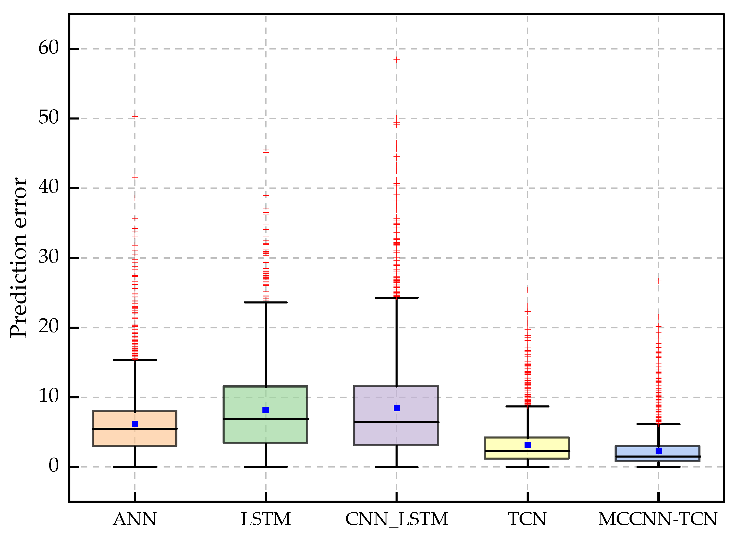
. It can be seen from Table 12 that the MAPE of the MCCNN-TCN model is 13.24%, which is 14.09%, 25.13%, 27.32%, and 4.48% higher than that of the ANN, LSTM, CNN-LSTM, and TCN models, respectively. The RMSE of the MCCNN-TCN model is 4.92 kW, which is also significantly less than that of other models. The absolute prediction error boxplots of the five models on the test dataset are shown in Figure 8. The wider the boxplot, the more spread out the prediction errors are. It can be seen from Figure 8 that the prediction error range of the MCCNN-TCN model is the narrowest while the LSTM is the widest, and the median absolute error of the MCCNN-TCN model is smaller than that of ANN, LSTM, CNN-LSTM, and TCN. From the prediction results, the MCCNN-TCN model is more effective than the ANN, LSTM, and CNN-LSTM models in complex fluctuation time series prediction.

In addition, it can be seen from Appendix A Figure A2 that in different seasons, the charging load of EVs will show different characteristics. Therefore, this means that the performance of the model proposed in this paper needs to be evaluated further during each season. According to the four seasons defined by meteorology, spring is from March 2019 to May 2019, summer is from June 2019 to August 2019, autumn is from September 2019 to November 2019, and winter is from December 2019 to February 2020. In this paper, each season’s historical load and meteorological data are selected, respectively, and the training set, the verification set, and the test set are selected according to the ratio of 8:1:1. The prediction errors of different models on the test set of each season are presented in

Table 13. Comparison of forecasting errors of models in each season.

	Spring			Summer			Fall			Winter
	RMSE/kW	MAE/kW	MAPE/%	RMSE/kW	MAE/kW	MAPE/%	RMSE/kW	MAE/kW	MAPE/%	RMSE/kW	MAE/kW	MAPE/%
ANN	14.67	10.93	36.86	18.04	13.22	24.44	17.74	13.51	20.27	11.50	8.68	31.52
LSTM	13.09	9.88	32.22	20.41	14.73	28.04	18.34	14.10	24.80	11.95	9.41	35.17
CNN-LSTM	13.24	9.84	29.97	20.37	15.13	26.45	19.17	14.29	21.81	12.30	9.28	33.29
TCN	8.03	6.12	20.90	9.97	7.34	13.55	8.66	6.42	10.05	5.75	4.22	16.01
MCCNN-TCN	6.36	4.45	14.24	8.96	6.25	10.80	7.49	5.32	7.53	5.29	3.78	13.65

.

As shown in Table 13, by comparing the prediction results of the five models in each season, the advanced nature of the model proposed in this paper can be verified intuitively. Although the prediction performance of each prediction model is different in different seasons, the MCCNN-TCN model proposed in this paper has a significant decrease in MAPE, RMSE, and MAE compared with other models in each season. By taking the spring test set as an example, compared with other models, the MAPE of the MCCNN-TCN model decreased by 22.62%, 17.98%, 15.73%, and 6.66%, and the MAE decreased by 6.48, 5.43, 5.39, and 1.67, respectively. In addition, on the test set of each season, the RMSE, MAE, and MAPE of the MCCNN-TCN model and the TCN model are smaller than those of other models. However, since the TCN model does not have the characteristics of multi-time scale feature extraction, its RMSE, MAE, and MAPE in each season are higher than those of the MCCNN-TCN model. Additionally, the MCCNN-TCN model’s mean absolute error is relatively concentrated and much lower than the other models under each season, as illustrated in Figure 9. Comparing the prediction results on the test set for each season demonstrates that the MCCNN-TCN model proposed in this paper has a stable prediction performance. This shows that the MCCNN-TCN model can adapt to the load forecasting demand of each season in a year and has good robustness and engineering application value.

4. Discussion

By comparing with the single-channel 1DCNN-TCN model, it can be demonstrated that the method of extracting EV charging load feature information at different time scales by setting multiple parallel 1DCNN passes can significantly improve the short-term load prediction performance.

The results in Table 12 show that the MCCNN-TCN model can effectively improve short-term load prediction by using an approach that extracts EV charging load features at multiple scales and relies on TCN to establish long-time dependencies between features. The ANN model has the disadvantage of only establishing superficial nonlinear mapping relationships, which leads to a weaker ability to extract temporal correlations of EV charging loads. Recurrent neural network models such as LSTM have memory properties. They can learn long-term temporal correlations, but feature extraction is weak due to the lack of convolution in their models. This leads to its poor effectiveness in predicting EV charging loads characterized by substantial fluctuations over short periods. The TCN model has superior predictive capabilities over the LSTM and CNN-LSTM due to the availability of convolutional units for extracting shallow temporal features and establishing temporal dependencies. However, the TCN model can only extract features at a single scale, and therefore its prediction performance is poorer than that of the MCCNN-TCN. Further, the results in Table 13 show that the predictive performance of the MCCNN-TCN model proposed in this paper is stable and outperforms those of the comparison models under different seasons.

Combined with the above analysis, it can be seen that the EV charging load prediction model proposed in this paper has a high prediction accuracy. However, the model proposed in this paper relies on the accuracy of meteorological data and EV charging load data to achieve high accuracy prediction. Therefore, some problems need to be noted in the engineering application of this method. On the one hand, if there are deviations in the meteorological data measurement of the forecasting day, this will affect the selection of similar daily loads. This paper uses several meteorological and date factors as day features when selecting similar day loads. Additionally, the adjacent day loads of the forecasting day to be measured are also added to the similar day set, making the similar day selection model somewhat fault-tolerant. On the other hand, in the power system, there are disturbances in the power load data from the measurement system caused by errors in the electric power system, outliers due to data encoding errors, and EV charging start and end times falling between load sampling points. Suppose the deviation from the actual value is slight. In that case, the deviation from the actual value obtained from the prediction model will also be slight. Conversely, suppose there are significant deviations from the actual values. In that case, the actual values need to be estimated using data pre-processing techniques such as mean-fill, interpolation, and algorithmic mean filtering.

5. Conclusions

Due to the randomness of EV charging behavior, the short-term fluctuation characteristics of EV charging load are obvious in one day. In order to improve the load prediction accuracy, this paper proposes the MCCNN-TCN load model, which considers the multi-time scale characteristics of EV charging loads. The multi-channel 1DCNN model was used to extract the features of EV charging load at multiple time scales. The TCN model was used to establish global temporal dependencies between the features.

By considering the influence of various factors on the load, MIC and Spearman coefficient were used to reduce the meteorological feature dimension and establish the similarity of date types, respectively. Then, taking the selected meteorological features and the similarity of date types as the daily features, a similar day selection model based on the weighted grey correlation degree was established to select similar daily loads. The selected meteorological features, date features, and similar daily loads were used as the input of the MCCNN-TCN model.

From the comparative experiments of single-channel 1DCNN-TCN and MCCNN-TCN, it can be seen that MCCNN-TCN can improve the prediction accuracy of EV charging load. This shows that the prediction performance can be improved by extracting the feature information of time series at different time scales and establishing global time series dependencies.

According to the prediction results compared with ANN, LSTM, CNN-LSTM, and TCN models, compared with these models, due to the unique structure of the MCCNN-TCN network, it can learn the multi-scale features of the EV charging load time series and master the changing law of EV charging load.

The MCCNN-TCN network constructed in this paper also lacks the consideration of real-time electricity price factors. In the future, we can further consider the selection of richer feature data and take advantage of big data to improve the accuracy of load forecasting.

References

1. Tribioli, L. Energy-Based Design of Powertrain for a Re-Engineered Post-Transmission Hybrid Electric Vehicle. Energies 2017, 10, 918. [Google Scholar] [CrossRef] [Green Version]
2. Habib, S.; Khan, M.M.; Abbas, F.; Sang, L.; Shahid, M.U.; Tang, H. A Comprehensive Study of Implemented International Standards, Technical Challenges, Impacts and Prospects for Electric Vehicles. IEEE Access 2018, 6, 13866–13890. [Google Scholar] [CrossRef]
3. Crozier, C.; Morstyn, T.; McCulloch, M. The opportunity for smart charging to mitigate the impact of electric vehicles on transmission and distribution systems. Appl. Energy 2020, 268, 114973. [Google Scholar] [CrossRef]
4. Lyu, L.; Yang, X.; Xiang, Y.; Liu, J.; Jawad, S.; Deng, R. Exploring high-penetration electric vehicles impact on urban power grid based on voltage stability analysis. Energy 2020, 198, 117301. [Google Scholar] [CrossRef]
5. Wang, H.; Yang, J.; Chen, Z.; Li, G.; Liang, J.; Ma, Y.; Dong, H.; Ji, H.; Feng, J. Optimal dispatch based on prediction of distributed electric heating storages in combined electricity and heat networks. Appl. Energy 2020, 267, 114879. [Google Scholar] [CrossRef]
6. Jiang, Y.; Yin, S. Recursive Total Principle Component Regression Based Fault Detection and Its Application to Vehicular Cyber-Physical Systems. IEEE Trans. Ind. Inform. 2018, 14, 1415–1423. [Google Scholar] [CrossRef]
7. Salah, F.; Ilg, J.P.; Flath, C.M.; Basse, H.; Dinther, C.V. Impact of electric vehicles on distribution substations: A Swiss case study. Appl. Energy 2015, 137, 88–96. [Google Scholar] [CrossRef]
8. Arias, M.B.; Bae, S. Electric vehicle charging demand forecasting model based on big data technologies. Appl. Energy 2016, 183, 327–339. [Google Scholar] [CrossRef]
9. Taylor, J.; Maitra, A.; Alexander, M.; Brooks, D.; Duvall, M. Evaluation of the impact of plug-in electric vehicle loading on distribution system operations. In Proceedings of the 2009 IEEE Power & Energy Society General Meeting, Calgary, AB, Canada, 26–30 July 2009. [Google Scholar]
10. Bae, S.; Kwasinski, A. Spatial and Temporal Model of Electric Vehicle Charging Demand. IEEE Trans. Smart Grid. 2012, 3, 394–403. [Google Scholar] [CrossRef]
11. Shun, T.; Kunyu, L.; Xiangning, X.; Jianfeng, W.; Yang, Y.; Jian, Z. Charging demand for electric vehicle based on stochastic analysis of trip chain. IET Gener. Transm. Distrib. 2016, 10, 2689–2698. [Google Scholar] [CrossRef]
12. Chen, T.; Zhang, B.; Pourbabak, H.; Kavousi-Fard, A.; Su, W. Optimal Routing and Charging of an Electric Vehicle Fleet for High-Efficiency Dynamic Transit Systems. IEEE Trans. Smart Grid 2018, 9, 3563–3572. [Google Scholar] [CrossRef]
13. Xing, Q.; Chen, Z.; Zhang, Z.; Huang, X.; Leng, Z.; Sun, K.; Chen, Y.; Wang, H. Charging Demand Forecasting Model for Electric Vehicles Based on Online Ride-Hailing Trip Data. IEEE Access 2019, 7, 137390–137409. [Google Scholar] [CrossRef]
14. Taylor, J.W. Short-Term Load Forecasting with Exponentially Weighted Methods. IEEE Trans. Power Syst. 2012, 27, 458–464. [Google Scholar] [CrossRef]
15. Hong, T.; Wilson, J.; Xie, J. Long Term Probabilistic Load Forecasting and Normalization with Hourly Information. IEEE Trans. Smart Grid. 2014, 5, 456–462. [Google Scholar] [CrossRef]
16. Zhang, J.; Wei, Y.; Li, D.; Tan, Z.; Zhou, J. Short term electricity load forecasting using a hybrid model. Energy 2018, 158, 774–781. [Google Scholar] [CrossRef]
17. Khodayar, M.; Liu, G.; Wang, J.; Mohammad, E.K. Deep learning in power systems research: A review. CSEE J. Power Energy Syst. 2021, 7, 209–220. [Google Scholar]
18. Xu, X.; Liu, W.; Xi, Z.; Zhao, T. Short-term load forecasting for the electric bus station based on GRA-DE-SVR. In Proceedings of the 2014 IEEE Innovative Smart Grid Technologies—Asia, Kuala Lumpur, Malaysia, 20–23 May 2014. [Google Scholar]
19. Yi, Z.; Liu, X.C.; Wei, R.; Chen, X.; Dai, J. Electric vehicle charging demand forecasting using deep learning model. J. Intell. Transp. Syst. 2021, 1–14. [Google Scholar] [CrossRef]
20. Zhu, J.; Yang, Z.; Chang, Y.; Guo, Y.; Zhu, K.; Zhang, J. A novel LSTM based deep learning approach for multi-time scale electric vehicles charging load prediction. In Proceedings of the 2019 IEEE Innovative Smart Grid Technologies, Chengdu, China, 21–24 May 2019. [Google Scholar]
21. Zhu, J.; Yang, Z.; Guo, Y.; Zhang, J.; Yang, H. Short-Term Load Forecasting for Electric Vehicle Charging Stations Based on Deep Learning Approaches. Appl. Sci. 2019, 9, 1723. [Google Scholar] [CrossRef] [Green Version]
22. Feng, J.; Yang, J.; Li, Y.; Wang, H.; Ji, H.; Yang, W.; Wang, K. Load forecasting of electric vehicle charging station based on grey theory and neural network. Energy Rep. 2021, 7, 487–492. [Google Scholar] [CrossRef]
23. Dabbaghjamanesh, M.; Moeini, A.; Kavousi-Fard, A. Reinforcement Learning-Based Load Forecasting of Electric Vehicle Charging Station Using Q-Learning Technique. IEEE Trans. Ind. Inform. 2021, 17, 4229–4237. [Google Scholar] [CrossRef]
24. Krizhevsky, A.; Sutskever, I.; Hinton, G.E. ImageNet classification with deep convolutional neural networks. Commun. ACM 2017, 60, 84–90. [Google Scholar] [CrossRef]
25. Li, Y.; Huang, Y.; Zhang, M. Short-Term Load Forecasting for Electric Vehicle Charging Station Based on Niche Immunity Lion Algorithm and Convolutional Neural Network. Energies 2018, 11, 1253. [Google Scholar] [CrossRef] [Green Version]
26. Ozcanli, A.K.; Yaprakdal, F.; Baysal, M. Deep learning methods and applications for electrical power systems: A comprehensive review. Int. J. Energy Res. 2020, 44, 7136–7157. [Google Scholar] [CrossRef]
27. Shang, C.; Gao, J.; Liu, H.; Liu, F. Short-Term Load Forecasting Based on PSO-KFCM Daily Load Curve Clustering and CNN-LSTM Model. IEEE Access 2021, 9, 50344–50357. [Google Scholar] [CrossRef]
28. Yan, K.; Wang, X.; Du, Y.; Jin, N.; Huang, H.; Zhou, H. Multi-Step Short-Term Power Consumption Forecasting with a Hybrid Deep Learning Strategy. Energies 2018, 11, 3089. [Google Scholar] [CrossRef] [Green Version]
29. Wei, L. A Hybrid Model Based on ANFIS and Empirical Mode Decomposition for Stock Forecasting. J. Econ. Bus. Manag. 2015, 3, 356–359. [Google Scholar] [CrossRef] [Green Version]
30. Zheng, H.; Yuan, J.; Chen, L. Short-Term Load Forecasting Using EMD-LSTM Neural Networks with a Xgboost Algorithm for Feature Importance Evaluation. Energies 2017, 10, 1168. [Google Scholar] [CrossRef] [Green Version]
31. Wang, Y.; Gu, Y.; Ding, Z.; Li, S.; Wan, Y.; Hu, X. Charging Demand Forecasting of Electric Vehicle Based on Empirical Mode Decomposition-Fuzzy Entropy and Ensemble Learning. Autom. Electr. Power Syst. 2020, 44, 114–121. [Google Scholar]
32. Wang, X.; Mao, D.; Li, X. Bearing fault diagnosis based on vibro-acoustic data fusion and 1D-CNN network. Measurement 2021, 173, 108518. [Google Scholar] [CrossRef]
33. Heo, S.; Nam, K.; Loy-Benitez, J.; Yoo, C. Data-Driven Hybrid Model for Forecasting Wastewater Influent Loads Based on Multimodal and Ensemble Deep Learning. IEEE Trans. Ind. Inform. 2021, 17, 6925–6934. [Google Scholar] [CrossRef]
34. Wang, Y.; Chen, J.; Chen, X.; Zeng, X.; Kong, Y.; Sun, S.; Guo, Y.; Liu, Y. Short-Term Load Forecasting for Industrial Customers Based on TCN-LightGBM. IEEE Trans. Power Syst. 2021, 36, 1984–1997. [Google Scholar] [CrossRef]
35. Yin, L.; Xie, J. Multi-feature-scale fusion temporal convolution networks for metal temperature forecasting of ultra-supercritical coal-fired power plant reheater tubes. Energy 2022, 238, 121657. [Google Scholar] [CrossRef]
36. Tang, X.; Chen, H.; Xiang, W.; Yang, J.; Zou, M. Short-Term Load Forecasting Using Channel and Temporal Attention Based Temporal Convolutional Network. Electr. Power Syst. Res. 2022, 205, 107761. [Google Scholar] [CrossRef]
37. Mishra, M.; Nayak, J.; Naik, B.; Abraham, A. Deep learning in electrical utility industry: A comprehensive review of a decade of research. Eng. Appl. Artif. Intell. 2020, 96, 104000. [Google Scholar] [CrossRef]
38. Korolko, N.; Sahinoglu, Z.; Nikovski, D. Modeling and Forecasting Self-Similar Power Load Due to EV Fast Chargers. IEEE Trans. Smart Grid 2015, 7, 1620–1629. [Google Scholar] [CrossRef]
39. Zhang, J.; Liu, D.; Li, Z.; Han, X.; Liu, H.; Dong, C.; Wang, J.; Liu, C.; Xia, Y. Power prediction of a wind farm cluster based on spatiotemporal correlations. Appl. Energy 2021, 302, 117568. [Google Scholar] [CrossRef]
40. Ge, L.; Xian, Y.; Wang, Z.; Gao, B.; Chi, F.; Sun, K. Short-term Load Forecasting of Regional Distribution Network Based on Generalized Regression Neural Network Optimized by Grey Wolf Optimization Algorithm. CSEE J. Power Energy Syst. 2020, 7, 1093–1101. [Google Scholar]
41. Reshef, D.N.; Reshef, Y.A.; Finucane, H.K.; Grossman, S.R.; McVean, G.; Turnbaugh, P.J.; Lander, E.S.; Mitzenmacher, M.; Sabeti, P.C. Detecting Novel Associations in Large Data Sets. Science 2011, 334, 1518–1524. [Google Scholar] [CrossRef] [Green Version]
42. Nascimento, J.; Pinto, T.; Vale, Z. Day-ahead electricity market price forecasting using artificial neural network with spearman data correlation. In Proceedings of the 2019 IEEE Milan PowerTech, Milan, Italy, 23–27 June 2019. [Google Scholar]
43. Han, M.; Zhang, R.; Qiu, T.; Xu, M.; Ren, W. Multivariate Chaotic Time Series Prediction Based on Improved Grey Relational Analysis. IEEE Trans. Syst. Man Cybern. Syst. 2019, 49, 2144–2154. [Google Scholar] [CrossRef]
44. An, L.; Teng, Y.; Li, C.; Dan, Q. Combined Grey Model Based on Entropy Weight Method for Long-term Load Forecasting. In Proceedings of the 2020 5th Asia Conference on Power and Electrical Engineering, Chengdu, China, 4–7 June 2020. [Google Scholar]
45. Song, J.; He, C.; Li, X.; Liu, Z.; Tang, J.; Zhong, W. Daily load curve clustering method based on feature index dimension reduction and entropy weight method. Autom. Electr. Power Syst. 2019, 43, 65–76. [Google Scholar]
46. Abdel-Hamid, O.; Mohamed, A.; Jiang, H.; Deng, L.; Penn, G.; Yu, D. Convolutional Neural Networks for Speech Recognition. IEEE ACM Trans. Audio Speech Lang. Process. 2014, 22, 1533–1545. [Google Scholar] [CrossRef] [Green Version]
47. Zhang, W.; Peng, G.; Li, C.; Chen, Y.; Zhang, Z. A New Deep Learning Model for Fault Diagnosis with Good Anti-Noise and Domain Adaptation Ability on Raw Vibration Signals. Sensors 2017, 17, 425. [Google Scholar] [CrossRef] [PubMed]
48. He, K.; Zhang, X.; Ren, S.; Sun, J. Deep residual learning for image recognition. In Proceedings of the 2016 IEEE Conference on Computer Vision and Pattern Recognition, Las Vegas, NV, USA, 27–30 June 2016. [Google Scholar]
49. Bai, S.; Kolter, J.Z.; Koltun, V. An empirical evaluation of generic convolutional and recurrent networks for sequence modeling. In Proceedings of the AAAI Conference on Artificial Intelligence, New Orleans, LA, USA, 2–7 February 2018. [Google Scholar]
50. Lore, K.G.; Stoecklein, D.; Davies, M.; Ganapathysubramanian, B.; Sarkar, S. A deep learning framework for causal shape transformation. Neural Netw. 2018, 98, 305–317. [Google Scholar] [CrossRef] [PubMed]
51. Xu, B.; Ye, H.; Zheng, Y.; Wang, H.; Luwang, T.; Jiang, Y.G. Dense Dilated Network for Video Action Recognition. IEEE Trans. Image Process. 2019, 28, 4941–4953. [Google Scholar] [CrossRef] [PubMed]
52. Farha, Y.A.; Gall, J. MS-TCN: Multi-stage temporal convolutional network for action segmentation. In Proceedings of the 2019 IEEE/CVF Conference on Computer Vision and Pattern Recognition, Long Beach, CA, USA, 15–20 June 2019. [Google Scholar]
53. Li, Y.; Huang, J.B.; Ahuja, N.; Yang, M.H. Joint imagefdiltering with deep convolu-tional networks. IEEE Trans. Pattern Anal. Mach. Intell. 2019, 41, 1909–1923. [Google Scholar] [CrossRef] [PubMed] [Green Version]
Figure 1. Multi-channel convolutional neural network and temporal convolutional network (Where, @ is preceded by the number of channels and followed by the output of the convolution layer).
Energies 15 02633 g001
Figure 2. Structure of one-dimensional convolutional neural network.
Energies 15 02633 g002
Figure 3. Multi-channel one-dimensional convolutional network.
Energies 15 02633 g003
Figure 4. Connection of multiple residual dilated causal convolution units.
Energies 15 02633 g004
Figure 5. Schematic of dilated causal convolution.
Energies 15 02633 g005
Figure 6. An illustration of the inputs and outputs of one residual dilated causal convolution unit.
Energies 15 02633 g006
Figure 7. Comparison of forecasting results of load models in 7 days.
Energies 15 02633 g007
Figure 8. Box plot of absolute prediction errors for different methods.
Energies 15 02633 g008
Figure 9. Box plot of absolute prediction errors for different methods in each season.
Energies 15 02633 g009