Modelling of Change in Fuel Mix within a District Heating Network

Abstract

Changing the fuel mix used in the heating industry, i.e., switching to greener fuels, is one of the possible solutions to prevent rising costs for final consumers in the context of rising emission allowance prices. This paper presents a methodology that offers the possibility to perform a comprehensive technical and economic assessment of a theoretical solution—changing the fuel mix of centralized heating sources—and other strategic decisions within a district’s heating systems. Emphasis is placed on fuels with a negative price, such as municipal waste. The presented approach can also be used to assess the effect of other significant changes related to the configuration of district heating systems on the economy of the plant, such as the impact of a decrease in heat demand and implementation of a steam turbine. The key benefit of this paper is an approach based on mathematical modelling of the operation of individual boilers with different operating parameters in terms of their start-up, shutdown, and mode of operation. A unique approach of optimizing an operation’s schedule using dynamic programming is presented, which enables the selection of a suitable solution for the configuration of binary variables in consecutive time steps. In this way, it is possible to achieve a more accurate estimate of the economics of the facility at the strategic planning stage that will consider the real operational capabilities of the heat source given its technical limitations. Using this approach, up to a 4% reduction in variable operating costs was achieved in the model case, when compared to static time interval planning.

1. Introduction

Increasing demands on the reduction of CO₂ emissions and other air pollutants put pressure on the greening of energy resources on a global scale. One of the areas that has significant consumption of fossil fuels is the heating industry, in which, in the conditions of the Czech Republic, energy production is mostly performed with coal or lignite, which have high emission factors. Compliance with stricter emission limits and an increase in the price of emission allowances create a need for additional investment in the heating industry and an increase in operating costs, which will have a negative impact on the price of heat for final consumers.

The global trend towards green energy necessitates the need for comprehensive changes, including the decarbonisation of energy resources. In addition to the economic aspects, the environmental aspects are also becoming topical [1]. The need for comprehensive modelling of energy dispatching, assuming the use of various fuels, including renewables, is closely related to this. This is necessary at the global, national, regional [2], and local levels. In the Czech Republic, a gradual shift away from coal combustion is currently underway. This phenomenon also applies to the heating industry. The reasons for this change are greening and decarbonisation, using tools such as emission allowances. As a result, the ever-increasing price of emission allowances also causes an increase in the final price of heat for consumers. To avoid rising prices, and thus the risk of a network breakdown, heating system operators are considering changing the used fuel mix. Currently, the price of emission allowances (February 2022) approaches the value of 100 EUR/t CO₂ and is still growing. In the Czech Republic, the average heat price for final consumers connected to district heating systems (DHS) is currently around 24 EUR/GJ [3]. With a CO₂ emission factor of lignite of 0.36 t CO₂/MWh [4] and a reference efficiency of separate heat production of 90% [5], the price of emission allowances represents approximately 24% of the final heat price. Given the current trends, a significant increase in this share can be expected.

The price of DHS heat for end customers must be regulated in some way to make this heat competitive compared to local heating [6]. This fact increases the demands on heating plant operators who, while maintaining acceptable costs and the resulting heat prices, must meet increasingly demanding emission limits. Preventing the breakdown of DHS is also strategically desirable from the state’s point of view, given the benefits and potential that centralized heat production offers. The Heat Roadmap Europe studies recommend expanding DHS to up to 50% of the total heat supply in Europe by 2050 [7].

The heating industry currently includes the obligation to surrender emission allowances for the combustion of fuels in plants with a total rated thermal input of more than 20 MW with the exception of plants for the incineration of hazardous or municipal waste [8]. However, in the future it is possible that this obligation will be extended to other sources as well. An option for reducing the variable operating costs arising from the surrender of emission allowances is the replacement of fuel by fuel with a lower emission factor (liquid fuels and natural gas (NG)) or by fuel that is not subject to emission allowances (biomass and municipal solid waste (MSW)). It should be noted here that emission allowances do not accurately reflect the actual CO₂ production of fuel combustion. In addition to the fact that some types of resources are currently entirely exempt from the payment of emission allowances, from the point of view of life cycle assessment (LCA), for example, the use of biomass for energy purposes is considered a renewable resource associated with a specific carbon footprint. Ilari et al. [9] performed an LCA analysis of a biomass power plant burning residual biomass in Italy. In this case, CO₂eq production was found to be reduced by 90.5% as compared to a reference fossil fuel plant.

In sensitivity analysis, Król and Ocłoń [10] investigated the impact of the increase in the price of emission allowances on the economy of a hybrid combined heat and power plant and emphasized the advantage of diversifying the fuel mix, where it is possible to use the most suitable fuel in energy production. Li et al. [11] emphasized the need for new energy development in China. In the authors’ previous work [12], up to 1.000 kg CO₂eq/t of MSW could be saved by replacing a fossil heat source with a waste-to-energy (WtE) plant. In the literature, there are optimization models for economic dispatch of combined heat and power (CHP) systems, which are used to plan the operation of existing facilities. For example, Kim et al. [13] introduced a tool for optimizing a complex CHP system in a case study using a neural network.

In this paper, a methodology that combines dispatch optimization and complex economic comparison of several potential technological variants is presented. This solution offers the possibility of assessing changing the fuel mix and other strategic decisions within the DHS, from an economic and environmental point of view. Some models consider the replacement of fossil fuels at the global or country level, such as [14]. However, the authors of this paper focus on the assessment of thermal energy production in a specific locality, where local aspects of the technology used are considered. Wang et al. The authors of [15] compared the used objective function, model type, form of energy export, and optimization method of cost-based optimal dispatch models of CHP plants.

The authors of this paper’s research objective was to create a universal methodology for the evaluation of investment plans in a specific locality with an existing heating plant delivering heat to a DHS, which would consider the basic parameters of all integrated technological units. In order to achieve this, a key part of the developed tool is the optimization model, which determines the economically optimal mode of operation of individual calculation variants in the first phase of the calculation. As further described in Section 2.3: Step 3—Technical and Economic Model, the main output of the tool is the change in the total cost of heat production, or the change in the heat price for customers, which is a key parameter in planning this type of project.

In contrast to other commonly used approaches, the parameters of existing heat sources and fluctuations in heat demand are considered, thus achieving a higher accuracy of estimating the economics of planned investments. Thanks to the versatility and flexibility of the created optimization model, it is possible that after minor modifications and data input it can be used for the evaluation of almost any DHS and to compare many possible variants.

The aim of this study is to include all the above-mentioned essential aspects in the optimization calculation. The presented approach principle consists of the mutual comparison of considered variants with the reference variant (typically the current state). Thanks to this approach, it is not necessary to know all of the data related to the economy, but only the data for which changes can possibly occur in the analysed variant. As a rule, these are the variable operating costs of the existing facility and potentially implemented technology, the investment costs of new technology, and a part of the fixed operating costs.

It is important to note that the subject of the research is the assessment of heat sources only up to the point of entry of the heating medium into DHS. There are references in the literature that offer a methodology for optimal design of pipeline networks in terms of minimizing investment costs, provided that the supply of heating medium to all end users is ensured [16].

2. Materials and Methods

This section presents in more detail the principle of evaluating the economics of investment plans in heating systems, which will then be presented in a case study. The whole methodology can be divided into three consecutive steps: “Step 1”, “Step 2” and “Step 3”. Step 1 includes the optimization model. This model aims to calculate the economically optimal mode of operation in a given technological solution during the year, while the calculation is performed at a standardized time each day. An economically optimal mode of operation can be defined as the state in which the difference between the variable operating costs (especially fuel costs) and revenues, depending on the operating mode (especially revenues from the sale of power), is minimal. Because the optimization model considers binary variables resulting from the operating mode of boilers and turbines, for each step of the calculation, there may be more results according to the currently set configuration. In previous work [12], the authors described the original mathematical model used to evaluate the economics of a WtE plant in detail. The key parameter that was evaluated was the acceptable price of heat at the foot of the WtE plant. This methodology was used in this paper, where it was extended by other technological concepts and subsequently linked with Step 2 and Step 3, thanks to which it was possible to compare different variants.

Step 2 consists of postprocessing of the results from Step 1, the aim of which is to select just one operation/shutdown configuration of calculation blocks with these binary variables. This phase of the calculation takes place in order to select a configuration that ensures the selection of a solution with minimal variable operating costs while respecting the requirements of the minimum required operating time or shutdown of these units. This step aims to estimate the critical economic parameters, which are directly dependent on the operation of the source: the variable operating costs and revenues, more specifically, their change compared to the reference variant.

In Step 3, the difference between the variable operating costs and revenues enters the balanced technical–economic model. In addition, it includes the change in fixed operating costs and investment costs. These are no longer dependent on the operating mode and are therefore not subject to optimization on shorter time periods. In this model, a final economic evaluation is performed, considering economic parameters such as inflation, discount rate, division of investment into depreciation classes, reinvestment in individual years, etc.

2.1. Step 1—Optimization

As mentioned above, Step 1 consists of the optimization calculation of the operation of the modelled technological variants and is implemented in MS Excel. The model is used to assess the future operation of the heating system in various configurations given by potential variants. The economically optimal operating mode is found here for a given configuration. Specifically, the difference between the variable costs and revenues from the sale of power is minimized, according to Equation (1):

$$n_t={\displaystyle \sum }_i\left(n_{var,i,t}-r_{i,t}\right),$$

(1)

where $n_t$ is the minimized the difference between the variable operating costs and revenues from electricity sales per day ($t$), $n_{var,i,t}$ are variable operating the costs of $i$-th boiler/turbine on day $t$, and $r_{i,t}$ are the revenues of the $i$-th boiler/turbine on day $t$.

The variables in the objective function of the optimization model described in this paper are considered to be purely economic. This means that the considered environmental aspect of CO₂ production is included here only in the form of the purchase of emission allowances, which increase the variable operating costs of heat sources. However, after modifying the code, it is possible to use multi-criteria optimization, in which the objective function could also be supplemented by LCA indicators such as global warming potential.

In this way, the operating costs of the individual variants are determined with the optimal use of the selected components. The model defines individual operating units, usually consisting of the boilers, steam turbines, and cogeneration units (CUs). The primary boundary condition is covering the heat demand in each period of time. The units are assigned their parameters, and the links between them are defined, i.e., the possible energy flows.

The calculation takes place at a time step of one day and in a series of 365 days in a row. The average thermal output of all components is selected for each day, which affects the balance of fuel consumption, energy production, and operating costs. An important factor is the limited flexibility of specific heat sources, which must be operated in a certain output range or completely shut down (e.g., solid fuel boilers). For example, Köfinger et al. [17] did not consider reducing the maximum heat output from the WtE plant concerning the integration with the biomass of the CHP plant. The solution that allows for the effective engagement of these sources, even with significantly fluctuating heat demand, is the use of thermal energy storage (TES) systems. Zhu and Li [18] presented a dispatch modelling methodology of CHP systems that considered the delayed response of the system to changes in heat demand. The following boundary conditions must be met during the calculation:

• Less flexible units (coal boilers) must be operated within their output range or shut down and must be in operation or downtime for a continuous period of time, e.g., at least one week;
• Coverage of heat demand in the modelled time period must be ensured;
• Steam turbines and CUs must be operated in the required power range or shut down.

Up to eight binary variables are currently included in the model, representing the operation/shutdown of boilers or steam turbines. This guarantees that the above boundary conditions are met. However, it should be noted that adding each binary variable currently doubles the computational time. For example, the current computational time of one variant using 8 binary variables is approximately 12 h on a standard desktop PC. It is essential to mention that by appropriate parallelization of the calculation or its implementation into the software directly intended for mathematical optimization, it would be possible to significantly reduce this time, which can be a subject of future work. When modelling the system, it is desirable to make simplifications that lead to the reduction in the number of blocks and thus the computational complexity. It is possible, for example, to combine several gas boilers into one unit due to the assumption that these sources are sufficiently flexible and the fact that the total operating costs are essential for economic evaluation; therefore, it is not necessary to differentiate individual boilers. The efficiency of all boilers is considered to be constant over the entire power range.

In addition to reducing the number of blocks and binary variables, an important factor is the requirement to maintain the linearity of the model to guarantee solvability in the optimization calculation. An example of this is the use of a linear characteristic in turbines. Steam turbine modelling is a complex problem [19], but analysis of operational data from existing WtE plants has shown that maintaining a linear characteristic allows for sufficient model accuracy.

A specific procedure was chosen for WtE plants, which act as heat sources with zero variable operating costs. Their economy can be therefore analysed further in the calculation in Step 2. Therefore, the use of this heat is always preferred over other sources. A particular emphasis was placed on WtE plants in the model. This technology is thought to have the potential to become the primary energy source in many localities [20]. This simplification can be done thanks to the assumption that MSW is a fuel with a negative price, and the given processing capacity is always used regardless of the current heat demand in the DHS. Therefore, the amount of steam corresponding to the given capacity is always available, and the variable operating costs of the WtE plant are constant, and it is not necessary to include them as a variable in the optimization calculation. An example of the input parameters in Step 1 is shown in

Table 1. Summary of input data to the first step of the calculation.

Technological Scheme	Parameters of Technological Units	Commodity Prices	Efficiencies	Heat Demand	Other Boundary Conditions
Boilers	Power range of boilers	Fuel prices	Efficiency of heat production in the boilers	Daily heat demand data at all levels	Pipe flow limitations
Steam turbines	Power range of turbines	Electricity price	Characteristics of steam turbines		Power output requirements
Cogeneration units	Shutdown options	Price of emission allowances			Technological energy consumption
Heat utilization		Other variable operating costs			Fuel emission factors
Definition of possible energy flows

.

A total of $2^x$ results representing the economically optimal mode of operation in each configuration is the output of the optimization for each day. $x$, in this case, indicates the number of binary variables used. The results include all combinations of binary variables. For example, if three binary variables are considered, there are 8 (2³) combinations of their operation/shutdown.

2.2. Step 2—Optimal Operations Schedule

The goal is not to have the optimal setup of the heating plant for one particular value of the parameters but rather to find the optimal schedule of operations throughout the year. Therefore, Step 1 is followed by postprocessing, in which suitable configurations of the operation of binary variables are selected for the individual days. This selection is based on two criteria: First, solutions that do not meet the boundary conditions are excluded. Second, the aim is to choose a configuration that ensures the minimum required continuous operation time or shutdown of individual boilers while ensuring minimum operating costs. For example, a situation where a solid fuel boiler would be in operation for only one day is excluded. This can be assessed using several different ways. The easiest way is to divide the modelled year into sections of a certain length. It is considered that individual technological units with less flexibility can be switched on/off only at the interface of these sections.

Within the methodology, a unique approach using dynamic programming (DP) was developed, presented on an example of technology with four lignite boilers, B1–B4, and a steam turbine, S, which cannot be turned on and off very frequently. This constraint is approached by modelling the operations of the plant in time as a discrete dynamical system with five states: $s_k^P$ for how long the part (P) in (P ∈ {B1, B2, B3, B4, S}) has been running at time $k$. The control then consists of five decisions $u_k^P$, which determine whether the part of the plant should be active (value 1) or inactive (value 0) at time$k$. The switch between the two values of $u_k^P$ can be made only after the corresponding part has been active for at least $m^p$ time units. It is possible to reduce the state space by mapping all of the states that correspond to the parts being active for a time longer than $m^P$ onto the state with a value of $m^P$. This reduction can be performed since the information that the corresponding part has been active for at least $m^P$ is sufficient to delimit the possible actions (i.e., the knowledge of how much longer that $m^P$ it has been active is not needed). The discrete dynamical system, with a fixed horizon, $N$, has ${\displaystyle \prod }_P\left(m^P+1\right)$ possible state values and can be described by the following Equations (2) and (3):

$$s_{k+1}^P=\left\{\begin{array}{cc}\hfill \max \left(s_k^P+1,m^P\right),& \hspace{1em}\hspace{1em}\mathrm{if} u_k^P=1\hfill \\ \hfill 0,& \hspace{1em}\hspace{1em}\mathrm{if} u_k^P=0\hfill \end{array}\right. k=0, 1, \dots ,N-1,$$

(2)

$$u_k^P\in U_k^P\left(s_k^P\right)=\left\{\begin{array}{c}1, \mathrm{if} s_k^P<m^P\\ \left\{0, 1\right\}, \mathrm{otherwise}\end{array}\right. k=0, 1, \dots ,N-1$$

(3)

The cost associated with each state $g_k\left(s_k, w_k\right)$ (with $s_k=\left[s_k^{B1}, s_k^{B2},s_k^{B3},s_k^{B4},s_k^P\right]$) corresponds to the optimal cost of the heating plant operations with the corresponding part being active or not (based on the value of the state). The control aims to find the optimal sequence of decisions ${\pi }^{*}=\left\{u_0^{*}, u_1^{*}, \dots , u_{N-1}^{*}\right\}$ (with $u_k^{*}=\left[u_k^{B1,*}, u_k^{B2,*}\right]$) that minimize the accumulated costs ($J^{*}$):

$${\pi }^{*}={\mathrm{argmin}}_{u_k;k=0,\dots ,N-1 } {\displaystyle \sum }_{k=0}^N{g}_k\left(s_k\right)$$

(4)

$$J^{*}={\min }_{u_k;k=0,\dots ,N-1 }{\displaystyle \sum }_{k=0}^N{g}_k\left(s_k,w_k\right)$$

(5)

Dynamic Programming

DP is one of the most widely used approaches for computing the optimal control for discrete dynamical systems [21], such as (2)–(5). Recently, it has been successfully employed for dynamic energy management of microgrids [22], optimal scheduling of electric bus fleets [23], energy management of electric vehicles [24], and operation strategies for grid-connected battery systems [25].

Based on the principle of optimality in dynamic programming, the optimal control for the discrete dynamic system can be solved by recursively computing the Bellman’s equation backwards in time as follows [21]:

$$J_N\left(s_N\right)=g_N\left(s_N\right)$$

(6)

$$J_k\left(s_k\right)=\underset{u_k\in U_k}{\min }{g}_k\left(s_k\right)+J_{k+1}\left(s_{k+1}\right),\hspace{1em}\hspace{1em}k=N-1,\dots , 0$$

(7)

For a given initial state $s_0$, the optimal expected cost $J^{*}$ is equal to $J_0\left(s_0\right)$. Moreover, if the minimizers of the right side of (6) $u_k^{*}=u_k^{*}\left(s_k\right)$ are collected for each $s_k$ and $k$, the optimal policy ${\pi }^{*}=\left\{u_0^{*}, u_1^{*}, \dots , u_{N-1}^{*}\right\}$ can be easily retrieved. Since the system equation is deterministic, the discrete dynamical problem can be reformulated into an equivalent graph problem [21]. In this reformulation, the states of the system correspond to nodes in the graph, while the edges describe the possible transitions from one state to another. The optimal control is then equivalent to finding the shortest path in the graph from a given starting state $s_0$ to any state $s_N$ in time $N$.

This solution will make it possible to find a suitable configuration of binary variables while meeting the boundary conditions. After the processing the output data from Step 1 in Step 2, the total annual values of significant parameters necessary for the overall economic evaluation of the project are calculated. These outputs are the operating mode of individual components for each time step of the calculation, variable operating costs of the considered variant, revenues from the sale of electricity, fuel consumption, power production, ash production, and emission production. The bold parameters are fundamental for the next calculation step (see Section 2.3).

The complete model works on the principle of comparing individual variants. Therefore, the calculation of Step 1 and Step 2 is performed twice—once for the reference variant (original state) and once for the calculation variant. By comparing the results, i.e., the variable operating costs and revenues before and after the considered change, the annual difference of these parameters is determined, which is a crucial parameter entering the Step 3 of the calculation.

2.3. Step 3—Technical and Economic Model

In Step 3, the results from the model in Step 1 (the annual variable operating costs and revenues from electricity sales) are used in another technical and economic model, which adds investments and fixed operating costs into the operating balance. Ferdan et al. [26] described the original version of this model. This model is purely balanced, as it does not include parameters subject to optimization (depending on the operating mode). Part of this model is a detailed WtE plant model, where the technology is modelled up to the point of energy export, which is already the input from Step 1.

The leading economic indicators of the individual variants are calculated, which are always related to the reference variant, i.e., in most cases to the current state, as mentioned above. This means that investment costs and operating variables as well as fixed costs and revenues do not enter Step 2 in absolute terms but instead in the form of the difference from the reference variant. Thanks to this approach, it is unnecessary to include the parameters common to all variants, such as revenues from heat sales or fixed operating costs. The main outputs from Step 2 are internal rate of return (IRR) of the variant at the end of the lifespan, net present value (NPV) of the variant at the end of lifespan and necessary increase or possible reduction of the heat price of heat to achieve NPV = 0 EUR at the end of the lifespan.

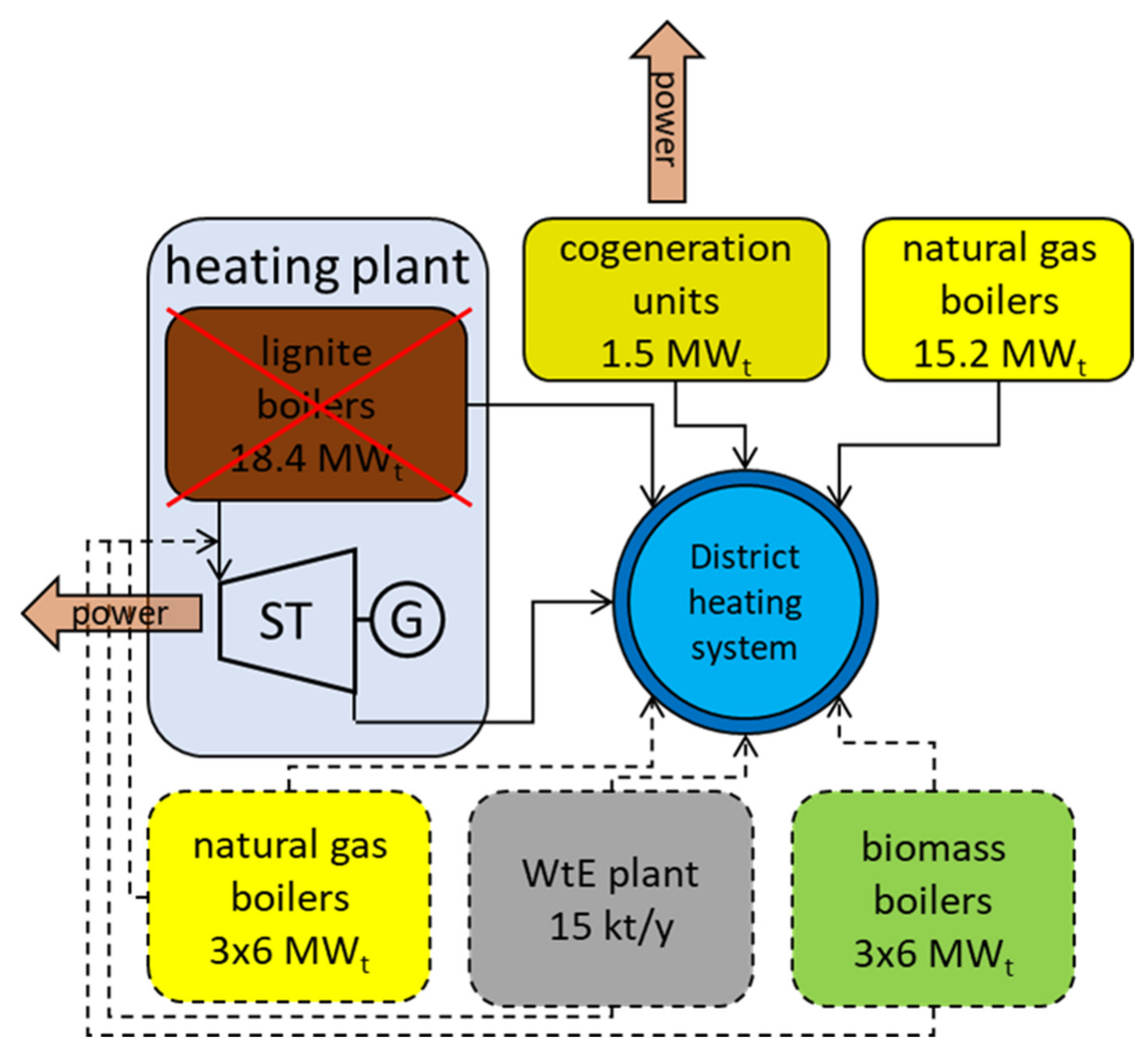
3. Case Study

The functions of the described tool are further described through a case study of an existing technology according to the diagram in Figure 1. The whole system consists of a heating plant with four lignite boilers with a total heat output of 18.4 MW_t with different parameters, two CUs with a total output of 1.5 MW_t, and several NG boilers with a total output of 15.2 MW_t. The heat is supplied to the DHS in the form of hot water heating with a total amount of 196 TJ/y. The heating plant produces cogeneration electricity in a back-pressure steam turbine but if necessary, it is possible to heat the water by heating it directly with live steam via a bypass. The operation of CUs is controlled remotely, does not depend on the current heat demand, and is considered to be constant throughout the year within daily cycles. NG boilers are available to cover peaks in demand and are used as a backup.

The optimization model, with respect to the reliability of the used input parameters, was verified during the modelling of operating states on the basis of the historical data of the reference variant. It was not possible to verify other calculation variants due to the fact that these are only hypothetical scenarios, but the input data were continuously consulted at the workplaces of the co-authors, who have been dealing with the considered technological concepts on a long-term basis.

The lignite boilers and the steam turbine represent binary variables that are expected to operate continuously or shut down for at least one week. For NG boilers, sufficient flexibility is assumed during start-up and shutdown, according to the current heat demand, which is simplified as zero minimum output in the model. Gas boilers can therefore be modelled as one virtual boiler. The same applies to the cogeneration units. The model of the current (reference) state, therefore, contains a total of 7 blocks (4 lignite boilers, CUs, NG boilers, and the steam turbine). For each day of the calculation, which is characterized by the heat demand for all configurations of binary variables, the economically optimal mode of operation was sought, provided that the boundary conditions were met (see Section 2.1 Step 1—Optimization). Thus, a total of 11,680 results were obtained for one year. In the future, decommissioning the lignite boilers and replacing them with another fuel is being considered. Three possible variants of the replacement were assessed, which were then compared with the reference variant. These variants were:

• Variant 1—construction of 3 × 6 MWt NG steam boilers;
• Variant 2—construction of a WtE plant with a processing capacity of 15 kt/y;
• Variant 3—construction of 3 × 6 MWt steam biomass boilers.

All these variants are considered steam and can supply heat directly to the DHS and the existing steam turbine. From the modelling point of view in Step 1, the considered new gas boilers are unified, the WtE plant acts as a boiler with zero variable operating costs (economy is assessed in Step 3), and biomass boilers are treated the same as the lignite boilers due to their lower flexibility.

4. Results

The principle is analogous for the calculation of all of the variants. First, the optimal mode of operation was calculated for each variant, each day, and each possible combination of binary variables individually within Step 1. Within Step 2, only one combination of binary variables was selected from the possible solutions using dynamic programming so that the solution meets the boundary conditions (see Section 2.2: Step 2—Optimal Operations Schedule).

A computational comparison of results with different values of $m^P$ (for simplicity, chosen to be the same for all parts) was performed.

Two control schemes, optimal by DP and “static”, where the time horizon of $N=365$ days, were segmented into time intervals of length $m^P$ (the last interval might be shorter). At each time interval, the parts of the plant that were active/inactive do not change and were chosen to minimize the costs (only regarding that time interval). Since for all parts, the value of $m^P$ was assumed to be the same, the static control was feasible (i.e., it satisfied the constraints (3)).

To better demonstrate the utility of using DP, random disturbances (from a uniform distribution) with variable magnitude were added to the costs.

Table 2. Optimal costs if there were no constraints on the $u_k^P$ (if one could switch the part of the heating plant on and off every day) for different magnitudes of added randomness. Average over 50 simulations.

	Added Randomness
	0%	5%	10%	15%
Cost EUR]	8.191 × 105	7.989 × 105	7.708 × 105	7.409 × 105

and

Table 3. Costs (EUR) for the static control and the optimal control of DP for different values of $m^P$ and different magnitudes of added randomness. Average over 50 simulations.

	Added Randomness
	0%		5%		10%		15%
${\mathit{m}}^{\mathit{P}}$	static	DP	static	DP	static	DP	static	DP
2	8.232 × 105	8.209 × 105	8.097 × 105	8.024 × 105	7.901 × 105	7.766 × 105	7.687 × 105	7.486 × 105
3	8.238 × 105	8.216 × 105	8.135 × 105	8.049 × 105	7.981 × 105	7.810 × 105	7.811 × 105	7.547 × 105
4	8.255 × 105	8.225 × 105	8.172 × 105	8.071 × 105	8.045 × 105	7.850 × 105	7.902 × 105	7.601 × 105
5	8.261 × 105	8.230 × 105	8.187 × 105	8.086 × 105	8.075 × 105	7.879 × 105	7.949 × 105	7.643 × 105
6	8.267 × 105	8.234 × 105	8.202 × 105	8.096 × 105	8.106 × 105	7.909 × 105	7.978 × 105	7.686 × 105
7	8.275 × 105	8.236 × 105	8.214 × 105	8.107 × 105	8.123 × 105	7.930 × 105	8.023 × 105	7.700 × 105

show the results.

Table 3 compares the achieved results of the minimum operating variable costs for different variants of added date for the static time interval and the interval using the DP method. It is evident that with larger variances of variable operating costs on individual days, the DP method reaches significantly different values than the static interval. Likewise, the difference in the resulting costs between the two methods differs more markedly at higher $m^P$. At 15% randomness, the deviation of both values depending on $m^P$ is from 2.6 to 4.0%.

In Figure 2, the results obtained by the DP (optimal states) of one simulation for $m^P=4$ are shown.

The yearly results of the calculation are summarized in

Table 4. Inputs to Step 3 of the calculation.

	Variant 0 (Reference)	Variant 1	Variant 2	Variant 3
Power sales (k EUR/y)	570.7	569.8	582.9	570.9
Variable operating costs (k EUR/y)	1.398.2	2.003.5	995.2	1387.2
Operating balance against the reference variant (k EUR/y]	0	606.2	−415.2	−11.2

. The key value is the balance of the difference between the variable operating costs and revenues from the sale of electricity as compared to the reference variant, which then enters Step 2 of the calculation. As already mentioned, since the methodology uses a comparison to the reference variant, it is unnecessary to include items that do not change within the individual variants in the operating balance, e.g., revenues from the sale of heat. The revenue from electricity sales varies across variants, but since electricity production is largely dependent on heat production, the differences are minimal. The variable operating costs differ significantly, as they depend mainly on the price of the fuel used and the impact of emission allowances (considered to be 40 EUR/t CO₂). In variant 1, the operating balance deteriorates due to more expensive fuel. In variant 2, there are savings since the fuel input (MSW) is not subject to optimization and enters as a fixed cost in Step 3. The values in the last line are then used as the virtual operating income in Step 3.

In Step 2, the overall economic balance of the assessed variants has already been performed. The used technical and economic model includes values from the last row of Table 4, which represent the annual balance of operating costs/revenues against the reference variant (in

Table 5. Calculation results.

	Variant 1	Variant 2	Variant 3
Balance of variable operating costs 1 (k EUR/y)	605.3	−403.0	−110.
Revenue balance 1 (k EUR/y)	−0.9	12.2	0.2
Investment costs 1 (k EUR)	−1.320	3240	2840
Fixed operating costs 1 (k EUR)	−233.4	391.9	−88
Necessary increase in the heat price to achieve IRR = 7.6% 1 (EUR/GJ)	+1.4	−0.1	+0.6
NPV 1 (k EUR)	−4.918	226	−1.656

¹ Against the reference variant.

divided into two rows). The fixed operating and investment costs are also included in this phase of the calculation, again in the form of the difference from the reference variant. In this way, it is possible to evaluate the economic impact of a change in the fuel mix as compared to the current state. For example, there is a negative difference in the investment costs for variant 1 when compared to the reference variant. The reason for this is that certain investments are needed while maintaining the reference variant, which, will not be reflected in other variants. Table 5 summarizes the basic inputs and outputs of Step 2. An internal rate of return (IRR) of 7.6% was requested by a potential investor.

The results show that variant 2 is the most economically advantageous, although it has the highest investment costs. The necessary increase in the price of heat is essentially zero and it can therefore be assumed that the implementation of this variant will maintain the price of heat for end consumers.

5. Discussion

A comprehensive model, using linear programming, was introduced to assess changing the fuel mix in heating plants. The presented methodology shows an increase in the accuracy of modelling the energy dispatch as compared to commonly used approaches found in the literature. A significant benefit of this paper is the creation of a methodology for the selection of binary variables in consecutive computational steps using dynamic programming. Thanks to this, it is possible to determine the economically optimal mode of operation of integrated facilities and at the same time to ensure compliance with the boundary conditions concerning the minimum operating time or shutdown of energy units.

The analysis showed that the operation planning of units with binary mode using dynamic programming allows for a significant reduction in variable operating costs if the heat demand fluctuates significantly between the individual time steps of the calculation. Conversely, if the heat demand is rather constant, this approach does not provide a significant increase in accuracy compared to simply dividing into identical time periods during the year.

While creating the described optimization model, the possibility of integration with WtE plants has been emphasized but the presented approach is also applicable to other strategic changes related to the configuration of DHS. The created tool can be used in dealing with real problems for industrial subjects such as:

• Economic assessment of WtE projects regarding the parameters of all sources supplying heat to the DHS;
• Multi-criteria evaluation of investment projects simultaneously from an economic and environmental point of view;
• Evaluation of the integration of various technological units, such as WtE plants, CUs, steam turbines or biomass boilers;
• Recommendation of an appropriate strategy for the planned fuel mix change and design of the optimal operation strategy of complex heating systems;
• Analysis of the sensitivity of energy sources to uncertain parameters.

The presented approach for technical and economic evaluation and the comparison of different variants of centralized heat sources in a particular locality is currently becoming particularly topical. The reason for this is the increasing emphasis on reducing CO₂ emissions, tightening emission limits on other pollutants, and problematic access to specific fuels.

The main advantage of the described approach, which was proven via practical application, is the possibility to easily perform economic comparison of a number of potential technological solutions. It was also very easy to assess the resilience of these options to changes in uncertain input parameters such as commodity price development.

6. Conclusions

The authors described a comprehensive tool using linear programming for technical and economic evaluation of investment plans in the field of energy sources supplying heat to DHS. The calculation itself consists of three consecutive steps: optimization calculation for the design of an economically optimal operation of a calculation variant, postprocessing to determine the appropriate combination of binary variables using the dynamic programming method, and a final balanced economic evaluation.

In particular, the optimization and the method of solving binary variables are the main novelties, described in more detail above, in comparison to simple balance models only. Using the principle of economic comparison with the reference variant, an economically optimal variant can be found, which enables the greening of the original source while maintaining an acceptable heat price for consumers.

Thanks to this approach, it is not necessary to include input parameters common to all calculation variants. The main results are the difference in the price of heat at the foot of the source and the total cost of its production.

In the final stage, the described approach was applied to an example of a real plant, where the replacement of coal boilers with another fuel was assessed with three variants: municipal solid waste, natural gas, and biomass. A special emphasis was placed on the design of the operation of the facility for which a binary mode of operation is assumed (either shutdown or operation in the given power range). In this step, a sensitivity analysis of the dependence of the increase in the accuracy of the model on the rate of fluctuation in heat demand was performed.