Abstract
The vibration signals for offshore wind-turbine high-speed bearings are often contaminated with noises due to complex environmental and structural loads, which increase the difficulty of fault detection and diagnosis. In view of this problem, we propose a fault-diagnosis strategy with good noise immunity in this paper by integrating the two-dimensional convolutional neural network (2DCNN) with random forest (RF), which is supposed to utilize both CNN’s automatic feature-extraction capability and the robust discrimination performance of RF classifiers. More specifically, the raw 1D time-domain bearing-vibration signals are transformed into 2D grayscale images at first, which are then fed to the 2DCNN-RF model for fault diagnosis. At the same time, three procedures, including exponential linear unit (ELU), batch normalization (BN), and dropout, are introduced in the model to improve feature-extraction performance and the noise immune capability. In addition, when the 2DCNN feature extractor is trained, the obtained feature vectors are passed to the RF classifier to improve the classification accuracy and generalization ability of the model. The experimental results show that the diagnostic accuracy of the 2DCNN-RF model could achieve 99.548% on the CWRU high-speed bearing dataset, which outperforms the standard CNN and other standard machine-learning and deep-learning algorithms. Furthermore, when the vibration signals are polluted with noises, the 2DCNN-RF model, without retraining the model or any denoising process, still achieves satisfying performance with higher accuracy than the other methods.
1. Introduction
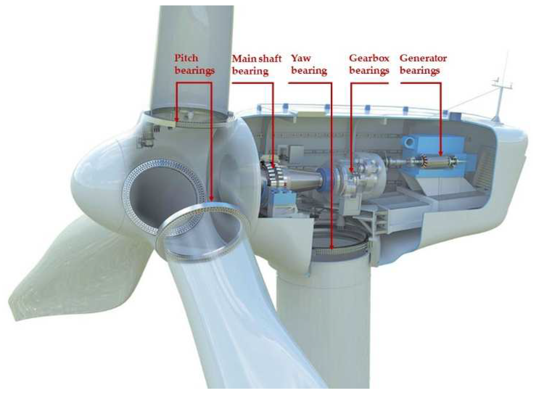
Wind energy has seen significant development in the past decade and is currently the most promising renewable energy resource. Notably, offshore wind turbines have better wind resources and wide operating space for large turbines than onshore ones. However, due to the harsh offshore environment, the failure rate of offshore wind turbines is much higher than that of onshore ones [1], which is an essential factor for the high cost of offshore wind energy. It has been observed there is a high failure rate of bearings in wind-turbine drivetrains as well as pitch-and-yaw systems, as shown in Figure 1. These bearings are continuously affected by alternating impact forces and loads from complex wind and wave environments, in which mechanical faults may occur. Therefore, advanced fault detection is required for evaluating the operating conditions of the bearings, so that maintenance can be implemented timely before catastrophic faults happen, and the operation and maintenance costs for offshore wind energy can be reduced [2].

Figure 1.
Bearings installed in wind-turbine drive systems.
There has already been a large amount of research work conducted for bearing-fault diagnosis based on vibration-signal analysis [3]. The traditional bearing-fault diagnosis process using vibration signals can be divided into two procedures, i.e., feature extraction and pattern recognition, and these two steps significantly affect the diagnosis results. When mechanical faults occur in the bearing, its vibration signal varies accordingly, leading to the energy change in each frequency band. Therefore, time–frequency-domain analysis methods have been used to extract time–frequency features, including fast Fourier transform (FFT), short-time Fourier Transform (STFT), wavelet transform (WT), variational mode decomposition (VMD), Wigner–Ville distribution (WVD), empirical mode decomposition (EMD), and ensemble empirical mode decomposition (EEMD) [4]. After feature extraction, pattern recognition is often used to diagnose and classify faults, such as support-vector machines (SVM), backpropagation neural networks (BPNN), Bayesian classifiers, and nearest-neighbor classifiers [5]. Many integrated bearing-fault diagnosis strategies have been proposed based on these algorithms [6,7]. Chen X et al. proposed an approach based on VMD-SVM for identifying bearing-fault types [8]. Long J et al. used the STFT method to analyze the wind-turbine bearing-vibration signals, and experimental results suggested that STFT had a high recognition rate and managed to extract fault characteristics [9]. Wang et al. used the improved tunable Q-factor wavelet transform (TQWT) with ensemble EEMD to extract the fault features of bearings [10]. Samanta B. et al. [11] used SVM for gear-fault classification, which showed better training time and classification accuracy than artificial neural networks. In [12], BPNN was used to locally learn meaningful and dissimilar features from signals of different scales, thus improving fault-diagnosis accuracy. Cheng et al. proposed a FFBRB (fuzzy fault-tree analysis and belief-rule base) model based on the Bayesian network, fuzzy fault-tree-analysis mechanism, and projection covariance-matrix-adaptation evolutionary strategies [13]. However, these aforementioned schemes based on manual feature extraction have the shortcomings of noise rejection. More specifically, vibration signals from rolling bearings are usually nonstationary and nonlinear. They are easily affected by complex operating conditions and background noises, increasing the difficulty of fault diagnosis with traditional methods based on manual feature extraction.
With the development of machine-learning techniques, many researchers have proposed to analyze the collected vibration data using learning-based approaches. For instance, a bearing-fault diagnosis approach based on long short-term memory (LSTM) was developed for wind-turbine fault prediction, and good efficiency, accuracy, and generalization ability were demonstrated [14]. Liang et al. proposed a method based on the kernel extreme learning machine (KELM) and whale optimization algorithm (WOA), and experimental results showed high classification accuracy and efficiency [15]. As a classical algorithm in ensemble learning, random forest (RF) is often used with other feature-extraction methods for classifications [16]. Rong et al. proposed a fault-diagnosis method for large-scale wind turbines, which combined CEMD and RF for multidomain fault diagnosis [17]. Fuzzy logic (FL) could also be used for fault diagnosis by partitioning the feature space into fuzzy sets, and a novel fuzzy-neural data-fusion engine was proposed for online monitoring and diagnosis [18]. Still, the performance of these fault diagnostic methods significantly relies upon the quality of artificial feature extraction. In addition, the vibration signals of the high-speed bearing of the offshore wind turbines are greatly affected by the noise interference caused by external disturbances, resulting in the difficulty of feature extraction.
Fortunately, deep learning, one of the essential subfields of machine learning, has been developed rapidly in the past few years, which is shown to be able to automatically extract and select features from data. Researchers have proposed to use deep-learning methods to process bearing-fault signals in the last few years. Nguyen et al. proposed a novel fault-diagnosis method using the deep neural network (DNN) [19], where the bearing-vibration signals were transformed into multiple-domain images and fed into a DNN with a multibranch structure, achieving good feature-extraction results. Jiang et al. proposed a multiscale CNN, which could extract fault features directly from the measured vibration signals of wind turbines [20]. In [21], a CNN-based gearbox-fault-diagnosis algorithm was proposed, which utilized the features in the time–frequency domain as the input of CNN to realize fault identification. Zhang et al. proposed a 1DCNN-PSO-SVM model for fault diagnosis [22], and experimental results suggested that this method could effectively extract the fault features of the wind-turbine gearbox. Zhang et al. proposed an improved Mask R-CNN model to automatically perform the fault detection for the wind-turbine bearings [23]. However, the above-mentioned classifiers are still influenced by measurement noises. If a robust classifier that incorporates mechanisms to be less influenced by noises could be combined with DNN, more robust fault-diagnosis results could be obtained.
In this paper, we propose a two-dimensional convolutional neural network (2DCNN) model for offshore wind-turbine high-speed bearing-fault diagnosis under noisy environments, which is supposed to utilize both CNN’s automatic feature-extraction capability and the robust discrimination performance of RF classifiers. First, the raw 1D bearing-vibration signals are converted into 2D grayscale images without information loss. Then, a 2DCNN-RF model is established to deal with these 2D images. In particular, three procedures, including batch normalization (BN), exponential linear unit (ELU), and dropout, are introduced in the model in order to improve the feature-extraction performance and noise immune capability. In addition, when the 2DCNN feature extractor is trained, the obtained feature vectors are sent to the RF classifier to improve the classification accuracy and generalization ability of the model. In order to verify the effectiveness of the proposed method, two groups of tests were conducted based on public high-speed bearing-vibration dataset, and the results were comparatively evaluated with other existing fault-diagnosis methods.
The remainder of this paper is organized as follows. Section 2 introduces the related theory of CNN and RF. Section 3 presents the proposed fault-diagnosis method based on the 2DCNN-RF model. Experimental results and comparative analysis are presented in Section 4. The conclusions are drawn in Section 5.
2. Related Theoretical Background
This section introduces the mathematical theories of CNN and RF which will be used in establishing the proposed fault-diagnosis model.
2.1. Convolutional Neural Network
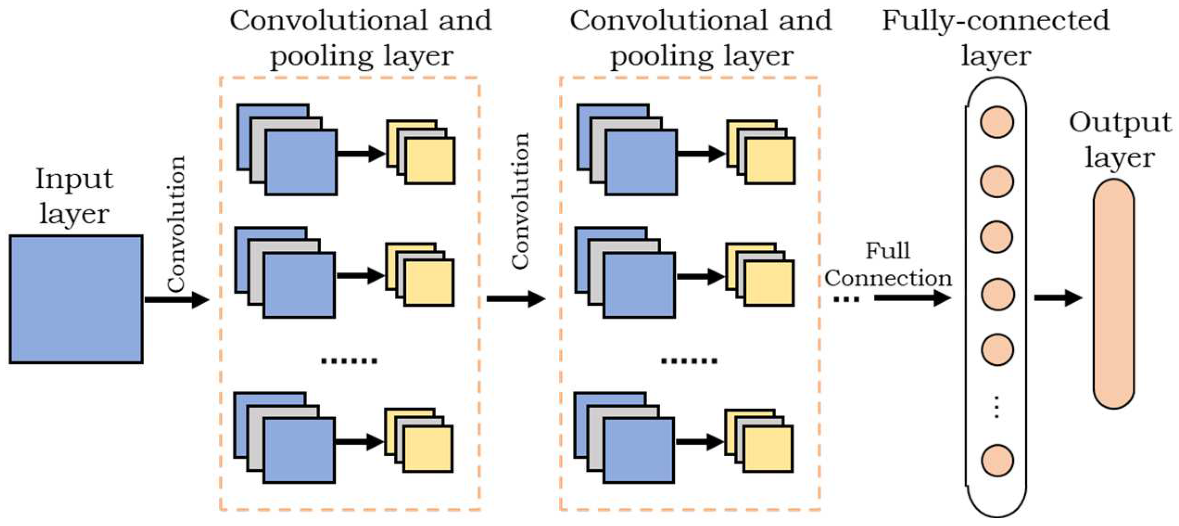
CNN was first proposed by LeCun for digital image processing, which was inspired by the principle of cell perception in the brain’s visual cortex [24]. CNN is composed of the convolution layer, activation layer, pooling layer, fully-connected layer, and output layer. The typical convolutional network structure is illustrated in Figure 2.
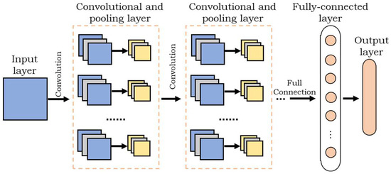
Figure 2.
Classical structure of CNN.
Mathematically, the formulas of each layer can be represented as follows:
- (1)
- Convolutional layer:where refers to the convoluted region on the layer and is its element. is the convolution output value of the channels on . and represent the weight and the bias of the channels on the layer, respectively.
- (2)
- Activation layer:where represents the activation function, such as the function, function, Heaviside activation function, and Rectified Linear Unit (ReLU) function.
- (3)
- Pooling layer:where is the downsample rule, which represents different types of pooling processes such as max pooling, average pooling, logarithmic pooling, and weight pooling. denotes the pooling window sliding with a particular stride, correspond to the pooling window’s dimension. is the activation map of the filter on the layer. represents the overlap between the pooling window and .
- (4)
- Fully connected layer:where is the feature vector, denotes the weight matrix, is the bias vector, and refers to the input vector. is the activation function.
- (5)
- Output layer:where m is the number of the labeled datasets, represents the loss function, and is the estimated output of CNN. is the fine-tuned parameters’ weight vectors and bias , which are obtained by minimizing the loss function [25].
2.2. Random Forest
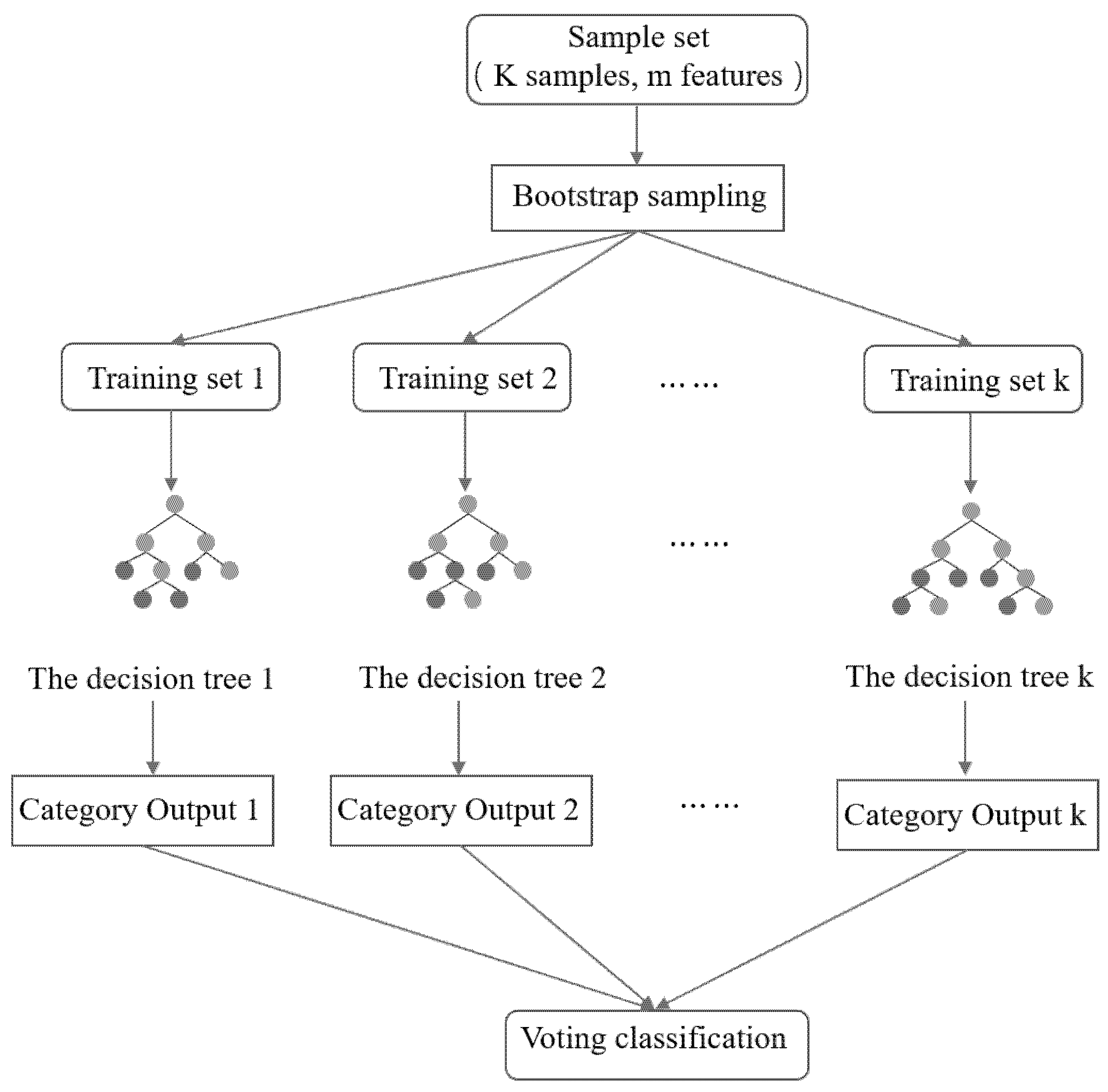
As one of the most popular ensemble-learning methods, random forest (RF) was first proposed by Leo Breiman, and is a statistical method used for regression and classification problems. The basic principle of RF is to construct a multitude of decision trees in the training process and produce output by combining the estimation of each tree [26].
As shown in Figure 3, based on the original training set, bagging, also known as bootstrap aggregating, is performed to generate a new training dataset for each decision tree. Bagging has the advantage of reducing variance within a noisy dataset [12]. The detailed RF-classification steps are listed as follows:
- (1)
- According to bootstrap, generate training subsets through random sampling with replacement.
- (2)
- Randomly select 𝑀 characteristic attributes from the characteristic attributes of one bootstrap sample and build a decision tree according to the CART algorithm [27].
- (3)
- Repeat Step (1) and Step (2) and establish decision trees.
- (4)
- Determine the final classification result by voting on the results of decision trees.

Figure 3.
Schematic diagram of random forest classifier.
Figure 3.
Schematic diagram of random forest classifier.
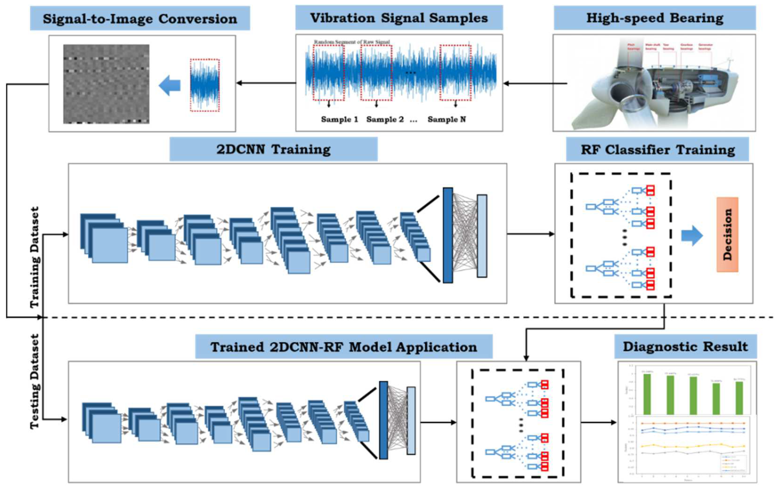
3. 2DCNN-RF Fault-Diagnosis Method
The proposed fault-diagnosis framework for the high-speed bearing of offshore wind turbines under noisy environments is based on the combination of CNN and RF. Figure 4 illustrates the overall diagram of the proposed fault-diagnosis method, which includes the following three steps. For the first step, bearing datasets are preprocessed by converting the raw 1D time-domain vibration signals into 2D gray-level images. Secondly, the 2DCNN model is trained based on the 2D grayscale-image training dataset, and then the obtained feature-extraction outputs will be used to train the RF classifier. In this step, a 2DCNN-RF model is learned through repeated training. Then, the trained 2DCNN-RF model is tested, utilizing the testing datasets to evaluate fault-diagnosis performance. Detailed steps of the proposed 2DCNN-RF model are listed in Algorithm 1.
| Algorithm 1 Steps of the implementation of the improved 2DCNN-RF model: |
| Input: Bearing-vibration-signal dataset |
| Output: The classification results and evaluation results of the 2DCNN-RF fault-diagnosis model. |
| Step 1: Dataset Preparation |
| Use the signal-to-image conversion method to convert the original 1D time-domain vibration signal into 2D grayscale images, which are then divided into the training dataset and testing dataset. |
| Step 2: Training the 2DCNN |
| 2.1 Initialize the scaling parameters and bias parameters of the conventional lay-ers and the fully connected layers randomly; |
| 2.2 Input a batch of the training dataset to the four-layer convolution-pooling structures for feature extraction and outputting feature maps; |
| 2.3 Input these feature maps to the fully connected layer that outputs the feature vector; |
| 2.4 Repeat (2.2)–(2.3) until the performance loss converges, and complete the training process; |
| 2.5 Extract the feature vectors from the trained 2DCNN. |
| Step 3: Training the RF classifier |
| 3.1 Input the extracted feature vectors to train the RF classifier; |
| 3.2 Output the classification results of the RF classifier. |
| Step 4: Verifying the fault-diagnosis performance of the proposed method |
| Verify the performance of the proposed method with the test dataset, and present the accuracy and efficiency results. |

Figure 4.
The flowchart of the proposed 2DCNN-RF scheme.
3.1. Vibration Signal-to-Image Transformation
CNN is constructed by imitating a biological visual-perception mechanism, so it is more suitable for learning features from the 2D images. To achieve better diagnosis performance, the raw 1D time-domain vibration signals are transformed into 2D grayscale images. The benefits of this 1D-2D transformation is that it does not require noise suppression, and no signal information is lost. The process of the vibration signal-to-image conversion is shown in Figure 5.
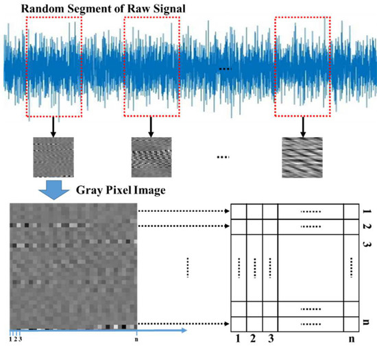
Figure 5.
The process of the vibration signal-to-image transformation.
Firstly, a signal segment is selected from the continuous raw data. Then, it is converted into a gray matrix image of dimension size image. is the pixel strength of the image, that is calculated by
where represents the rounding function, which is used to set the image pixel grayscale as an integer between 0 to 255.
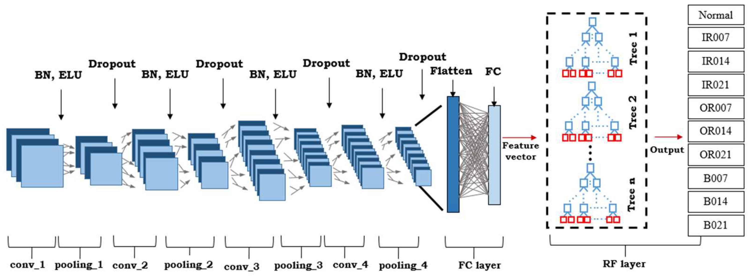
3.2. Design of the Proposed 2DCNN-RF Model
As illustrated in Figure 6, the structure of the proposed 2DCNN-RF model combines the CNN feature extractor and the RF classifier. It contains four-layer convolution-pooling structures, a fully connected layer, and an RF layer. After converting the vibration signals into 2D grayscale images, four-layer convolution-pooling structures are used for feature extraction. To alleviate the effect of gradient exploding and overfitting and to improve the 2DCNN feature-extraction performance under a noisy environment, three procedures, including batch normalization (BN), exponential linear unit (ELU), and dropout, are introduced in the model. When the 2DCNN feature extractor is trained, the obtained feature vectors will be passed to the RF as a new training dataset for learning and classification.
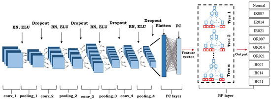
Figure 6.
Structure of the proposed 2DCNN-RF model.
To prevent the gradient vanishing/exploding during network training, the BN layer can also prevent overfitting and improve training speed. The BN layer is calculated by
where is the output map of the BN layer, and denotes the input with the average value of and standard deviation of , and is a small positive number for numerical stability. The scaling parameter and bias parameter are learnable parameters in BN layers.
In addition, we also applied the exponential linear unit (ELU) to the ReLU function in order to shorten the training time and improve accuracy in neural networks. Moreover, as a nonsaturating activation function, ELU does not encounter the gradient vanishing/exploding problem. The ELU function is defined as
where represents a small positive value.
The structure of the 2DCNN is also optimized by dropout, which can significantly reduce overfitting by randomly discarding a defined percentage of neurons. The dropout layer can be used in each hidden layer in training CNN in each training batch. Following the convolutional layer, the dropout layer can increase the robustness to noise input, and the use of dropout after the fully connected layer can prevent from overfitting.
As shown in Figure 6, the feature-extraction outputs (128 values in our study) of 2DCNN are fed into the RF classifier for training. Once the RF classifier is well-trained, it performs the recognition task and makes decisions and outputs the classification results on high-speed bearing-fault diagnosis.
4. Experimental Results and Analysis
In order to evaluate the performance of the proposed fault-diagnosis approach, public experimental data from the high-speed bearing-test rig were used, and the test results were comparatively evaluated with other fault-diagnosis methods. Note that all the fault-diagnosis tests were carried out on a PC with Ryzen 7 4.5 GHz 8-Core AMD CPU and Nvidia RTX3060 GPU. The proposed 2DCNN-RF model was written in Python, and the famous deep-learning framework TensorFlow was employed to implement the algorithm.
4.1. Experimental Dataset
4.1.1. Dataset Description
Since the actual bearing-fault signals for offshore wind turbines are usually commercially private, the open dataset from the Bearing Data Center of Case Western Reserve University (CWRU) was used in this work to verify the proposed fault-diagnosis approach, which has similar rotational speeds to those of high-speed bearings for utility-scale wind turbines. The CWRU bearing dataset has been widely used for wind-turbine high-speed bearing-fault-diagnosis studies [28,29].
As shown in Figure 7, the test rig consists of a 2 hp motor, a torque transducer/encoder, and a dynamometer. Different loads, ranging from 0 hp to 3 hp, were applied to the shaft via a dynamometer and electronic control system. The rotation velocities of the motor varied from 1797 rpm to 1730 rpm. In the following experiments, the shaft rotating speed was 1772 r/min, which was similar to the high-speed bearing of an offshore wind turbine. Faults ranging in diameter from 0.18 to 0.71 mm were seeded on both the drive-end and fan-end bearings, using electrodischarge machining (EDM). Vibration data were collected using accelerometers, which were placed close to these bearings.
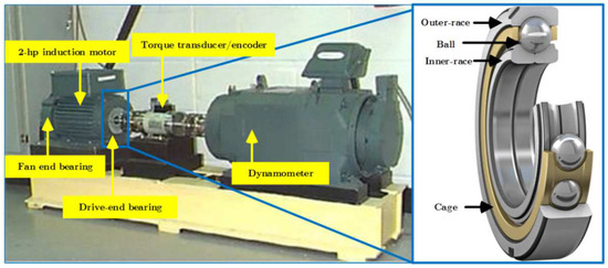
Figure 7.
Bearing test rig used for the experiment.
In this paper, vibration data with 12 kHz sampling frequency measured in the vertical direction on the housing of the drive-end bearing (DE) were used in the following experiments. Single-point damages on the ball, inner ring, and outer ring were introduced in the experiment, so there are four states for the bearing, i.e., normal state, ball-failure state, inner-ring-failure state, and outer-ring-failure state. The diameters of the faults created on the inner race, outer race, and the balls are 0.007, 0.014, and 0.021 inch, respectively. According to the fault states and fault diameters, the vibration data were classified into 10 types of working conditions. For each working condition, the data were divided into 1000 groups with 1024 sampling points in each group, and we used one-hot encoding to label the dataset of 10 working conditions. The detailed information of the dataset is presented in Table 1. The selection of the training dataset is random, and the ratio of training data to test data is 7 to 3.

Table 1.
Detailed information of the CWRU dataset.
4.1.2. DCNN-RF Model Architecture
Based on the proposed 2DCNN-RF model design in Section 3, several critical parameters need to be chosen, which are listed in Table 2.
Table 2.
Model-parameter table.
The selection of these parameters is problem-dependent and obtained by trial and error. A grayscale image with a size of 32 × 32 was fed into the 2DCNN-RF model, which was processed by the four-layer convolution-pooling structures, and 256 feature maps of 2 × 2 were obtained. Then, these extracted feature maps were flattened to a 1024-dimensional feature vector, which is used as the input of the fully connected layer. As mentioned above, dropout is introduced in the training process, and the dropout value is set to be 0.5. The BN layer is only employed after four convolutional layers, and their scaling parameters and bias parameters are initialized randomly. The RF classifier consisted of 100 decision trees in this case, and its output size was set as 10, corresponding to 10 different working conditions. In addition, the gradient-descent method was employed for training the deep-learning network with a training rate of 0.0001, and the training was carried out for 50 epochs.
4.2. Results and Discussions
In order to verify the noise immunity of the proposed fault-diagnosis method, two groups of experiments were conducted, including experiments on the original CRWU dataset and evaluations with various levels of noise added. Introducing the latter case is supposed to test the noise-resistive ability of the fault-diagnosis algorithms. Standard CNN, LSTM, BP, and SVM algorithms were also used for comparison in the testing.
4.2.1. Performance on the CRWU Dataset
In the first experiment, the training and testing datasets were randomly selected from the CRWU datasets, as shown in Table 1. Before being fed into the 2DCNN-RF model, each raw signal segment containing 1024 sample points was converted into a grayscale image with a size of using the signal-to-image conversion method. Figure 8 shows the resultant grayscale images for the four health states. Due to the limited space, only a set of conversion results for the normal state and faulty states with the inner ring, outer ring, and ball fault in 0.36 mm diameter are shown from Figure 8a–d.
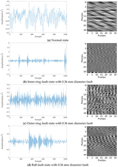
Figure 8.
Grayscale− image−conversion results for the four health states.
After the signal-to-image transformation and the 2DCNN-RF model construction, the training and testing procedures for fault diagnosis were implemented. We selected the four most commonly used evaluation indicators, i.e., Accuracy, Precision, Recall and F1-Score, to assess the fault-diagnosis performance of the proposed 2DCNN-RF model [30],
where TP is a true positive, FP is a false positive, TN is a true negative, and FN represents a false negative. Accuracy is the measurement for correct classification. Precision is used for estimating how many of the predicted samples are correctly detected. Recall evaluates how many positive labels are correctly predicted based on the original samples. F1-score is used to measure the overall performance.
The values of these three evaluation indicators for bearing-fault diagnosis under different working conditions are shown in Table 3. The averages of Accuracy, Precision, Recall and F1-Score values are 0.995, 0.995, 0.994, and 0.996, respectively, indicating that the model has good feature-extraction and fault-classification capabilities.
Table 3.
The values of evaluation indicators under different working conditions.
In addition, to comparatively evaluate the performance of the proposed 2DCNN-RF model, selected standard machine-learning algorithms, including BPNN and SVM, and standard deep-learning models, including CNN and LSTM, were also tested for comparison study [31,32]. The main parameters of the above standard learning methods are described as follows.
- Standard CNN with raw data: two-layer convolution-pooling structures are used. ReLU function is used as the activation function of the hidden layer.
- LSTM with eight features: LSTM neural network contains two LSTM layers. The Tanh function is seen as the activation function of the hidden layer.
- BPNN with nine features: Two hidden layers have 15 and 20 nodes, respectively. The Sigmoid function is used as the activation function of the hidden layer.
- SVM with eight features: RBF kernel is used. The penalty coefficient is set as 2, and the gamma value is set as 1.
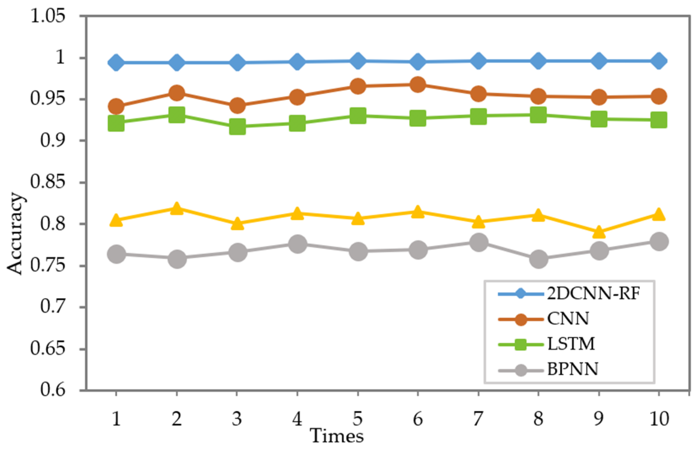
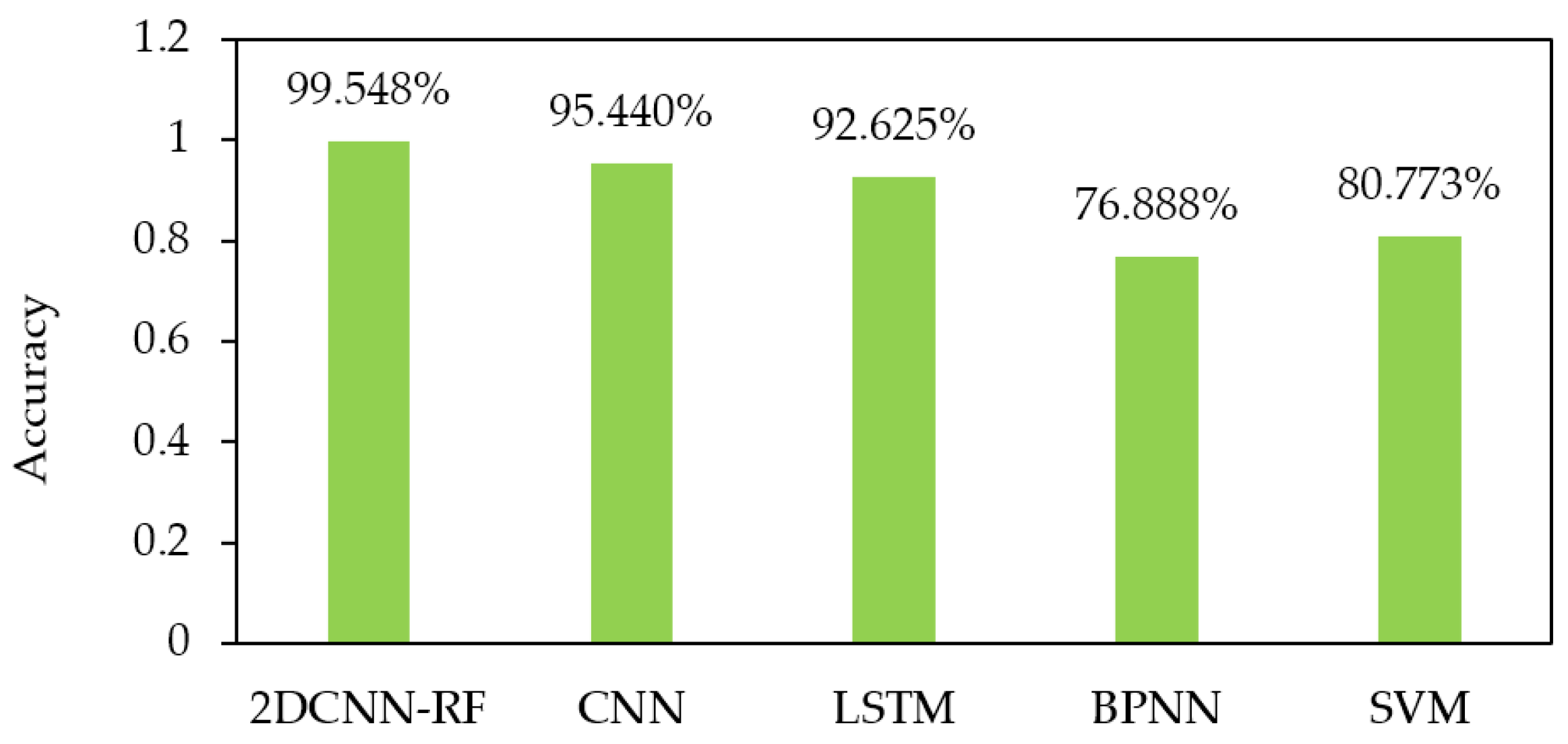
All the tests were conducted 10 times on the dataset listed in Table 1, and the fault diagnosis results are listed in Figure 9 and Figure 10, while the mean prediction accuracy is seen as the general evaluation indicator for this comparison. It can be seen that the average diagnostic accuracy of the proposed 2DCNN-RF model is 99.548%, which is better than those of other models. Compared with the standard CNN, the 2DCNN-RF model improves the diagnostic accuracy by 5%. Another deep-learning model, LSTM, has a diagnostic accuracy of 92%, since its diagnosis performance depends heavily on manual feature extraction. The accuracy of the BPNN and SVM are 76.88% and 80.773%, respectively, which are significantly worse than those of the deep-learning-based approaches. It can be seen that these machine-learning-based models cannot explore the inherent complex relationships between the fault features and the vibration signals.
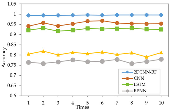
Figure 9.
Fault-diagnosis-accuracy comparison for different methods.
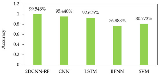
Figure 10.
The average accuracy of fault diagnosis for different models.
4.2.2. Performance on the CRWU Dataset with Noise Pollution
As mentioned above, offshore wind turbines are operating under complex environmental and structural loads, which could cause higher measurement noises, such as high-speed bearing-vibration signals. In order to further evaluate the noise immune ability of the proposed fault-diagnosis method, another test was performed based on the original CRWU with additional noises added. More specifically, Gaussian white noises were added to the CRWU high-speed bearing-vibration dataset to introduce the measurement noises [33]. The strength of the measurement-noise intensity is usually measured by the signal-to-noise ratio (SNR), which is defined by
where and denote the powers of the original signal and the additional Gaussian noises, respectively.
The larger the value of SNR, the smaller the noise contained in the vibration signals. SNR is inversely proportional to the amount of noise in the vibration signals. For example, we added Gaussian white noise with SNR = 0 dB to the vibration signal labeled IR014, collected from the inner ring with a fault diameter of 0.36 mm. The raw vibration signal, Gaussian white noise and noise-added signal are plotted in Figure 11a–c, while the grayscale images before and after adding noise are shown in Figure 12a–b, respectively.
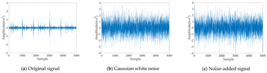
Figure 11.
Noiseadded vibration signal with SNR = 0 dB.
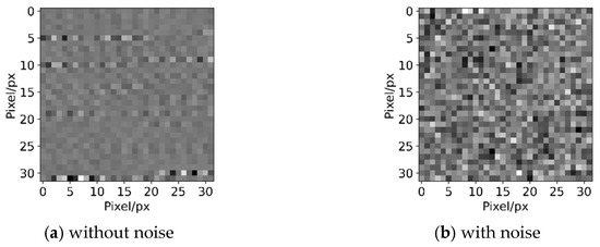
Figure 12.
The grayscale images before and after adding noise with SNR = 0 dB.
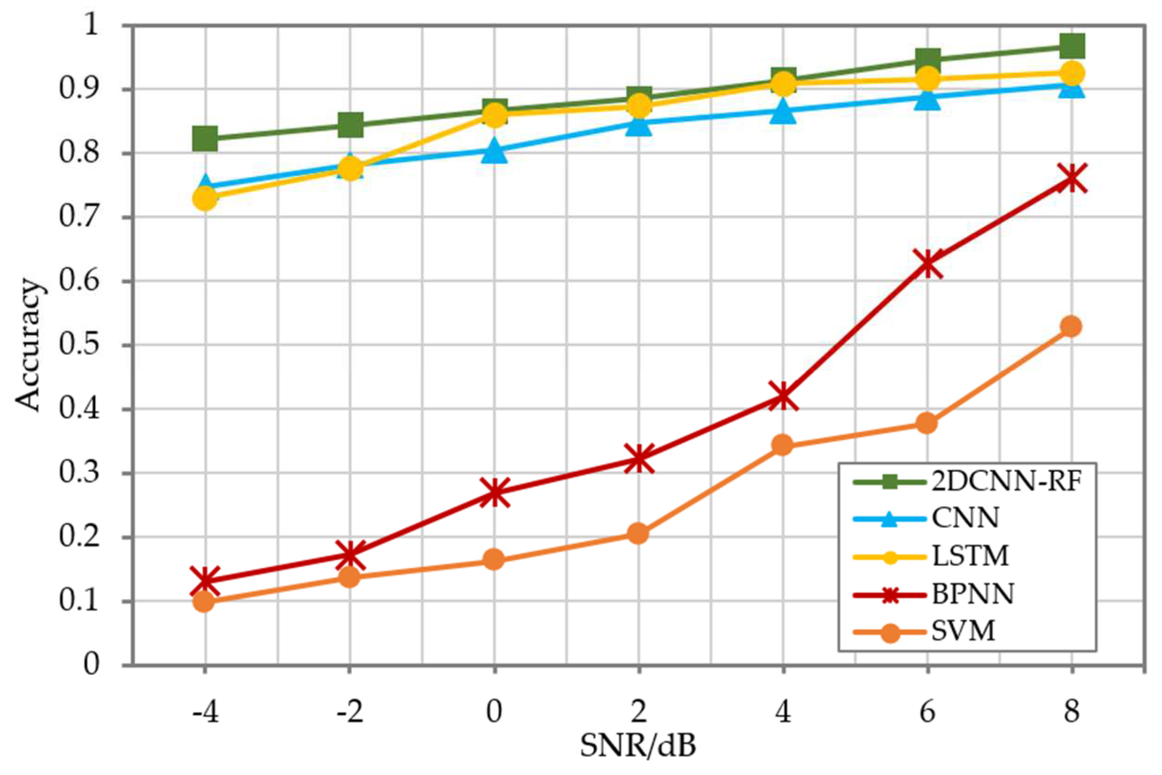
Different noise levels were tested by adding Gaussian white noises with SNR ranging from −4 dB to 8 dB to the original datasets described in Table 1. Then, the noise−added grayscale images and vibration signals were used as the input of 2DCNN−RF, standard CNN, LSTM, BPNN and SVM, so that their noise-resistive fault-diagnosis performance could be evaluated and compared. Figure 13 shows the fault-diagnosis accuracy of the five fault-diagnosis models. In comparison with Figure 9, Figure 13 shows that the fault-detection accuracy was reduced for all fault−diagnosis methods by introducing the additional measurement noises, which means a high noise level will pose a risk of fault-detection failure. Moreover, it can be observed that the fault-diagnosis accuracy will decrease with increasing noise intensity for all methods, and the noise impact on machine-learning methods is more significant than that of deep-learning methods. Still, the proposed 2DCNN−RF has better accuracy than the other four models. Under noise condition SNR = −4dB, the diagnostic accuracy of the 2DCNN−RF model still reaches 80.26%, which is 5% higher than that of the standard CNN and LSTM models. The accuracy of machine learning methods, namely BPNN and SVM, is only about 10%. These evaluation results demonstrate that the proposed 2DCNN-RF fault-diagnosis strategy is more robust against noise pollution for high-speed bearing-vibration signals.

Figure 13.
Performance comparison under different noise conditions.
5. Conclusions
Since the vibration signals of offshore wind-turbine high-speed bearings are often polluted by noises due to complex environmental and structural loads, a novel fault-diagnosis strategy based on the 2DCNN-RF model is proposed in this work to improve the fault-diagnosis accuracy and noise immunity. The main contribution of this study is the establishment of a 2DCNN-RF fault-diagnosis model by combining the 2DCNN feature extractor with the RF classifier, which is shown to be able to both improve the fault-diagnosis accuracy and noise-resistive capability. The proposed model was tested on the dataset from CWRU test rig. The experimental results show that the diagnostic accuracy of the 2DCNN-RF model could achieve 99.548% on the original CWRU dataset, which outperforms the standard CNN and other mainstream machine-learning-based and deep-learning-based methods. Furthermore, when the vibration signals are polluted with noises, the 2DCNN-RF model, without retraining the model or any denoising process, still achieves satisfying performance with higher accuracy than the other diagnostic methods. More specifically, under noise condition SNR = −4dB, the diagnostic accuracy of the 2DCNN-RF model still reaches 80.26%, which is 5% higher than that of the standard CNN and LSTM models. The accuracy of machine-learning methods, namely BPNN and SVM, is only about 10%. Thus, it is anticipated that the proposed method is suited for the implementation in high-speed bearing-fault diagnosis of offshore wind turbines under noisy environments. Experimental tests on offshore wind turbines are to be conducted in order to further validate the effectiveness of the proposed fault-diagnosis strategy in the future.
Author Contributions
Conceptualization, S.Y. and Y.S. (Yulin Si); methodology, Y.S. (Yulin Si); software, P.Y.; validation, W.F.; data curation, H.Y.and J.B.; writing—original draft preparation, S.Y.; writing—review and editing, Y.S. (Yulin Si) and Y.S. (Yuxiang Su); funding acquisition, Y.S. (Yulin Si) and S.Y. All authors have read and agreed to the published version of the manuscript.
Funding
This study is funded by National Natural Science Foundation of China, grant number 61903337 and 51705453, Key Research and Development Program of Zhejiang Province, grant number 2021C01150, Science and Technology Plan Project of Zhoushan Science and Technology Bureau, grant number 2020C21011 and 2019C81036, and Zhejiang Provincial Natural Science Foundation of China, grant number LQ18E070004.
Institutional Review Board Statement
Not applicable.
Informed Consent Statement
Not applicable.
Conflicts of Interest
The authors declare no conflict of interest.
References
- Si, Y.; Chen, Z.; Zeng, W.; Sun, J.; Zhang, D.; Ma, X.; Qian, P. The influence of power-take-off control on the dynamic response and power output of combined semi-submersible floating wind turbine and point-absorber wave energy converters. Ocean Eng. 2021, 227, 108835. [Google Scholar] [CrossRef]
- Ren, Y.; Vengatesan, V.; Shi, W. Dynamic Analysis of a Multi-column TLP Floating Offshore Wind Turbine with Tendon Failure Scenarios. Ocean Eng. 2022, 245, 110472. [Google Scholar] [CrossRef]
- Tandon, N.; Choudhury, A. A review of vibration and acoustic measurement methods for the detection of defects in rolling element bearings. Tribol. Int. 2000, 32, 469–480. [Google Scholar] [CrossRef]
- Huang, N.; Chen, Q.; Cai, G.; Xu, D.; Zhao, W. Fault Diagnosis of Bearing in Wind Turbine Gearbox Under Actual Operating Conditions Driven by Limited Data With Noise Labels. IEEE Trans. Instrum. Meas. 2020, 70, 1–10. [Google Scholar] [CrossRef]
- Wang, X.; Mao, D.; Li, X. Bearing fault diagnosis based on vibro-acoustic data fusion and 1D-CNN network. Measurement 2021, 173, 108518. [Google Scholar] [CrossRef]
- Guo, T.; Deng, Z. An improved EMD method based on the multi-objective optimization and its application to fault feature extraction of rolling bearing. Appl. Acoust. 2017, 127, 46–62. [Google Scholar] [CrossRef]
- Lu, W.; Wang, X.; Yang, C.; Tao, Z. A novel feature extraction method using deep neural network for rolling bearing fault diagnosis. In Proceedings of the The 27th Chinese Control and Decision Conference, Qingdao, China, 23–25 May 2015. [Google Scholar]
- Chen, X.; Yang, Y.; Cui, Z.; Shen, J. Vibration fault diagnosis of wind turbines based on variational mode decomposition and energy entropy. Energy 2019, 174, 1100–1109. [Google Scholar] [CrossRef]
- Long, J.; Wu, J.-Q. Application of Short Time Fourier Transform and Hilbert-Huang Transform in Fault Diagnosis of Rolling Bearings of Windmill. Noise Vib. Control 2013, 33, 219–222. [Google Scholar]
- Wang, H.; Jin, C.; Dong, G. Feature extraction of rolling bearing's early weak fault based on EEMD and tunable Q-factor wavelet transform. Mech. Syst. Signal Process. 2014, 48, 103–119. [Google Scholar] [CrossRef]
- Samanta, B. Gear fault detection using artificial neural networks and support vector machines with genetic algorithms. Mech. Syst. Signal Process. 2004, 18, 625–644. [Google Scholar] [CrossRef]
- Li, J.; Yao, X.; Wang, X.; Yu, Q.; Zhang, Y. Multiscale local features learning based on BP neural network for rolling bearing intelligent fault diagnosis. Measurement 2019, 153, 107419. [Google Scholar] [CrossRef]
- Cheng, X.; Liu, S.; He, W.; Zhang, P.; Xu, B.; Xie, Y.; Song, J. A Model for Flywheel Fault Diagnosis Based on Fuzzy Fault Tree Analysis and Belief Rule Base. Machines 2022, 10, 73. [Google Scholar] [CrossRef]
- Zou, P.; Hou, B.; Lei, J.; Zhang, Z. Bearing fault diagnosis method based on EEMD and LSTM. Int. J. Comput. Commun. Control 2020, 15. [Google Scholar] [CrossRef] [Green Version]
- Liang, R.; Chen, Y.; Zhu, R. A Novel Fault Diagnosis Method Based on the KELM Optimized by Whale Optimization Algorithm. Machines 2022, 10, 93. [Google Scholar] [CrossRef]
- Li, C.; Sanchez, R.V.; Zurita, G.; Cerrada, M.; Cabrera, D.; Vasquez, R.E. Gearbox fault diagnosis based on deep random forest fusion of acoustic and vibratory signals. Mech. Syst. Signal Process. 2016, 76-77, 283–293. [Google Scholar] [CrossRef]
- Jia, R.; Ma, F.; Dang, J.; Liu, G.; Zhang, H. Research on Multidomain Fault Diagnosis of Large Wind Turbines under Complex Environment. Complexity 2018, 2018, 2896850. [Google Scholar] [CrossRef] [Green Version]
- Wijayasekara, D.; Linda, O.; Manic, M.; Rieger, C. FN-DFE: Fuzzy-Neural Data Fusion Engine for Enhanced Resilient State-Awareness of Hybrid Energy Systems. IEEE Trans. Cybern. 2014, 44, 2065–2075. [Google Scholar] [CrossRef]
- Nguyen, V.-C.; Hoang, D.-T.; Tran, X.-T.; Van, M.; Kang, H.-J. A Bearing Fault Diagnosis Method Using Multi-Branch Deep Neural Network. Machines 2021, 9, 345. [Google Scholar] [CrossRef]
- Jiang, G.; He, H.; Yan, J.; Xie, P. Multiscale Convolutional Neural Networks for Fault Diagnosis of Wind Turbine Gearbox. IEEE Trans. Ind. Electron. 2019, 66, 3196–3207. [Google Scholar] [CrossRef]
- Chen, Z.; Li, C.; Sanchez, R.-V. Gearbox fault identification and classification with convolutional neural networks. Shock Vib. 2015, 2015, 390134. [Google Scholar] [CrossRef] [Green Version]
- Zhang, X.; Han, P.; Xu, L.; Zhang, F.; Gao, L. Research on Bearing Fault Diagnosis of Wind Turbine Gearbox Based on 1DCNN-PSO-SVM. IEEE Access 2020, 8, 192248–192258. [Google Scholar] [CrossRef]
- Zhang, J.; Cosma, G.; Watkins, J. Image Enhanced Mask R-CNN: A Deep Learning Pipeline with New Evaluation Measures for Wind Turbine Blade Defect Detection and Classification. J. Imaging 2021, 7, 46. [Google Scholar] [CrossRef] [PubMed]
- Li, X.; Zhang, W.; Ding, Q. Deep learning-based remaining useful life estimation of bearings using multi-scale feature extraction. Reliab. Eng. Syst. Saf. 2019, 182, 208–218. [Google Scholar] [CrossRef]
- Xu, G.; Liu, M.; Jiang, Z.; Söffker, D.; Shen, W. Bearing Fault Diagnosis Method Based on Deep Convolutional Neural Network and Random Forest Ensemble Learning. Sensors 2019, 19, 1088. [Google Scholar] [CrossRef] [PubMed] [Green Version]
- Breiman, L. Random Forests. Mach. Learn. 2001, 45, 5–32. [Google Scholar] [CrossRef] [Green Version]
- Hui, C. Strategy of selecting original configuration for satellite constellation using CART algorithm. J. Huazhong Univ. Sci. Technol. (Nat. Sci. Ed.) 2011, 39, 1–5. [Google Scholar]
- Xu, Z.; Li, C.; Yang, Y. Fault diagnosis of rolling bearing of wind turbines based on the variational mode decomposition and deep convolutional neural networks. Appl. Soft Comput. 2020, 106515. [Google Scholar] [CrossRef]
- Zareapoor, M.; Shamsolmoali, P.; Yang, J. Oversampling adversarial network for class-imbalanced fault diagnosis. Mech. Syst. Signal Process. 2021, 149, 107175. [Google Scholar] [CrossRef]
- Li, Y.; Jiang, W.; Zhang, G.; Shu, L. Wind turbine fault diagnosis based on transfer learning and convolutional autoencoder with small-scale data. Renew. Energy 2021, 171, 103–115. [Google Scholar] [CrossRef]
- Mushtaq, S.; Islam, M.M.; Sohaib, M. Deep Learning Aided Data-Driven Fault Diagnosis of Rotatory Machine: A Comprehensive Review. Energies 2021, 14, 5150. [Google Scholar] [CrossRef]
- Nakamura, H.; Mizuno, Y. Diagnosis for Slight Bearing Fault in Induction Motor Based on Combination of Selective Features and Machine Learning. Energies 2022, 15, 453. [Google Scholar] [CrossRef]
- Zare, S.; Ayati, M. Simultaneous fault diagnosis of wind turbine using multichannel convolutional neural networks. ISA Trans. 2020, 108, 230–239. [Google Scholar] [CrossRef] [PubMed]


Publisher’s Note: MDPI stays neutral with regard to jurisdictional claims in published maps and institutional affiliations. |
© 2022 by the authors. Licensee MDPI, Basel, Switzerland. This article is an open access article distributed under the terms and conditions of the Creative Commons Attribution (CC BY) license (https://creativecommons.org/licenses/by/4.0/).