Abstract
The engineering wind farm models currently used in industry can assess power losses due to turbine wake effects, but the prediction of power losses due to farm blockage is still a challenge. In this study we demonstrate a new prediction method of farm blockage losses and a possible strategy to mitigate them for a large offshore wind farm in the North Sea, by combining a common engineering wind farm model ’FLORIS’ with the ’two-scale momentum theory’ of Nishino and Dunstan (2020). Results show that the farm blockage losses depend significantly on the ’wind extractability’ factor, which reflects the strength of mesoscale atmospheric response. For a typical range of the extractability factor (assessed using a numerical weather prediction model) the farm blockage losses are shown to vary between about 5% and 15% of the annual energy production (AEP). However, these losses may be mitigated by adjusting turbine operating points taking into account the wind extractability. It is shown that a simple adjustment of the blade pitch angle and tip-speed ratio used below the rated wind speed may increase the AEP by up to about 2%.
1. Introduction
Wind energy is a key component of the global strategy of transition towards renewable energy. In 2021, wind energy made up 22.7% of the UK’s electricity generation, of which 63% was offshore wind [1]. As nations around the world set targets and make plans to increase their wind power production, power predictions for new offshore wind projects must be as accurate as possible. Ensuring accurate predictions enables a realistic picture of the future of wind energy production to be formed.
Two key aerodynamic effects in the prediction of wind farm performance are wake effects and farm blockage effects. These effects both act to cause a deceleration of flow and thus a reduction of power produced by turbines in a wind farm. Traditionally, wake effects have been thought to have a dominant influence on wind farm power production, so studies have been conducted to alleviate their impact, using turbine yaw control or ’wake steering’ [2], dynamic induction control [3,4] and different hub-heights [5,6], among others (see, e.g., [7] for a review of these topics). Recent studies have shown, however, that farm blockage effects may also significantly impact wind flow and hence power production, especially for large and dense wind farms [8,9].
The farm blockage effect (also known as the farm induction effect) is the effect caused by the presence of turbines in a wind farm as a whole. This causes a farm-scale induction, meaning that the wind speed upstream of an ’unwaked’ turbine in a wind farm (typically in the front row of a farm but this may also be in the middle of a farm) is slower than that of an isolated turbine. Some recent studies suggest that superposing individual turbine-scale inductions can be used to predict farm-scale induction [10,11]. For large wind farms, however, this cannot be predicted without considering the mesoscale atmospheric response which affects the momentum balance across an entire wind farm [12].
The main aim of this paper is to predict the impact of mesoscale atmospheric response on the power of a real-life large offshore wind farm, by using an existing engineering wind farm model ’FLORIS’ together with the two-scale momentum theory [9,13]. Following this, a new operation control method to reduce the impact of farm blockage on power production is also explored. Current control strategies used in the wind industry for turbine operating conditions (i.e., how the blade pitch and rotational speed should change with wind speed) do not take into account the farm blockage effect explicitly. A recent study by Lanzilao and Meyers [14] has explored this idea for an idealised wind farm with different atmospheric conditions, showing that the farm blockage effect could be mitigated to maximise the farm power by adjusting the farm thrust coefficient. This paper therefore aims to further explore this idea and quantify how much of the blockage-induced power loss for a real-life wind farm could be mitigated by re-optimising turbine operating conditions taking into account the farm blockage effect explicitly.
2. Theory
In this section we briefly summarise the two-scale momentum theory of Nishino and Dunstan [9] on which the present study is based. The “two-scale” nature of the theory comes from the fact that in this theory the problem of air flow over a large wind farm is split into two sub-problems. The ’external’ (farm-scale) problem is a time-dependent problem that considers large-scale motions of the atmospheric boundary layer (ABL). This is to assess the amount of momentum available to the bottom resistance of the ABL at a certain time. The ’internal’ (turbine-scale) problem is a quasi-steady problem that assesses the proportions of turbine drag and sea surface friction that make up the bottom resistance of the ABL. A parameter called the ’farm induction factor’ plays a key role in coupling the two sub-problems so that the farm-scale momentum balance equation outlined below can be solved analytically using information from both sub-problems.
2.1. Farm-Scale Momentum Balance
A control volume (CV) containing an entire wind farm is used for this analysis, as illustrated in Figure 1, to consider the farm-scale momentum balance for a short-time-averaged flow (i.e., the effect of turbulence is considered as Reynolds stresses). The height of the CV can be chosen arbitrarily, and all fluxes of streamwise momentum through the top and side surfaces of the CV (due to advection and Reynolds stresses) are implicitly included in the momentum availability factor, M (together with the effects of pressure gradient, Coriolis force and acceleration/deceleration of the flow inside the CV; see [9] for details). Then the non-dimensional farm momentum (NDFM) equation for this CV is
where
is a farm-averaged ’local’ or ’internal’ thrust coefficient of turbines, is the thrust of i-th turbine in the farm, n is the number of turbines, is the array density (A is the swept area of each turbine and S is the farm area), is the natural sea-surface friction coefficient (assumed to be 0.002 in this study), is the friction exponent (assumed to be 2 in this study), is the farm wind-speed reduction factor (and thus is the farm induction factor), and and are the ’farm average’ wind speeds for the cases with and without turbines, respectively (see Section 3.5 for more details). Note that the first term of the left hand side of Equation (1) shows how large the total turbine drag is relative to the natural sea-surface friction drag, and the second term represents how much the sea-surface friction drag differs from its natural value, whereas the right hand side (M) represents how much the available momentum differs from its natural value.
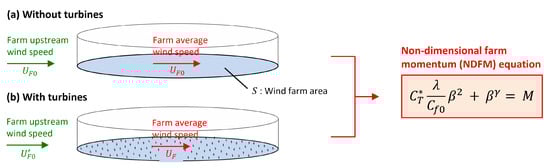
Figure 1.
Schematic of a control volume containing the whole area of a large offshore wind farm (for the case with and without turbines).
2.2. Wind Extractability
Following [9,12] we estimate the momentum availability factor M using a linear approximation model, defined as
where is called the momentum response parameter or “wind extractability” parameter, describing how the momentum available to the farm site changes with the farm-average wind speed. Note that represents a hypothetical situation where the momentum available to the farm site is fixed (i.e., ), whereas corresponds to another hypothetical situation where the farm-average wind speed never decreases from its natural value (i.e., ).
There are several factors that may affect the wind extractability. These include regional weather patterns, atmospheric stratification, height of the ABL and gravity waves [15]. For example, a recent study using a numerical weather prediction (NWP) model [12] suggests that, for a large (20 km-diameter) offshore wind farm off the east coast of Scotland, typically takes values between 5 and 25. In this study we consider three different values of 10, 15 and 20 as low, medium and high extractability scenarios (without considering any potential correlations between and wind speed or direction; such correlations may exist and should be investigated in future studies).
2.3. Power and Thrust Coefficients
The power and thrust coefficients of each turbine are defined as
where P is the turbine power, T is the turbine thrust, and is the incoming wind speed, i.e., streamwise velocity measured upstream of each turbine. In this study we employ an engineering wake model without considering the axial induction upstream of each turbine, which means that is simply the streamwise velocity averaged over the (upstream side of) rotor swept area. Note that Equation (5) can be used to calculate T from and for each turbine in the farm, and this can be used to calculate from Equation (2).
In this study we will compare three different modelling cases, which are referred to as Cases 0, A and B. In Case 0 we ignore the farm blockage effect (as in traditional studies using engineering wake models only); in this case, is the same as unless the turbine is in the wake of other turbines. In Case A and Case B, however, can be different from even for front-row turbines, since the wind speed upstream of the entire farm is adjusted such that the farm-scale momentum balance is satisfied. Further details of this adjustment are described later in Section 4.
3. Methodology
This section will describe the overall computational setup used in this study. We first describe a traditional load control strategy as this forms the basis of all three cases in this study (Cases 0, A and B). Methods specific to each case will be explained later in the relevant sections. We also describe the details of the wind turbines and wind farm considered, as well as the farm modelling tool used, in this section.
3.1. Load Control Strategy
The two main turbine conditions that are changed according to a traditional load control strategy are the tip speed ratio (TSR) and the blade pitch angle. Figure 2 shows the variations of these two parameters (as well as the resulting power, power coefficient and rotational speed) with the incoming wind speed, for a 10 MW wind turbine considered in Case 0 and Case A in this study.
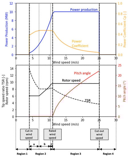
Figure 2.
Operating regions and variation of the power, rotor speed, pitch angle and TSR.
There are four regions of turbine operation for different wind speeds. In Region 1 (below the cut-in wind speed) there is no power produced, and the power coefficient is zero. Region 2 can be further divided into Regions 2a, 2b and 2c. These sub-regions can be best identified by looking at the rotor speed. In Regions 2a and 2c the rotor speed is fixed, whereas in Region 2b the rotor speed linearly increases with the wind speed (to maintain the optimum TSR that maximises the power coefficient). The blade pitch is kept constant throughout Region 2. At the start of Region 3, the rated power (10 MW) is reached, and the power production is capped at this value. In order to achieve this power capping, the blade pitch and TSR are adjusted to reduce the power coefficient as the wind speed increases. In Region 4 the cut-off wind speed is reached and there is no power production.
3.2. Wind Turbine
The turbine considered in this study is based on the DTU 10 MW turbine [16]. Table 1 summarises the key parameter values of the turbine used.

Table 1.
Summary of turbine parameters.
The and tables for the DTU 10 MW turbine (containing all and values corresponding to a range of pitch-TSR combinations) are available online [17]. The pitch values range from ° to 24.5°, and the TSR values range from 3 to 14.5, as demonstrated in the contour plots in Figure 3.
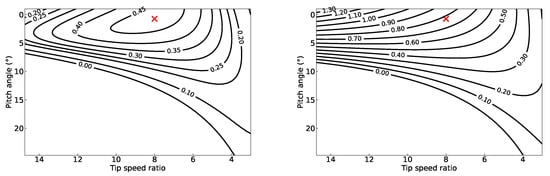
Figure 3.
Contour plots of (left) and (right) for the DTU 10 MW turbine. The marker on each plot shows the operating point for Region 2b of operation.
Power and thrust curves can be created from the and tables using the turbine operation conditions for the DTU 10 MW turbine [16], i.e., indexing the coefficients that correspond to the prescribed pitch-TSR combinations for a range of wind speeds. However, to follow the traditional load control strategy described earlier in Section 3.1, we modify the pitch-TSR combinations for Regions 2b and 3 of operation. For Region 2b (from 7 m/s to 10 m/s) the pitch angle and TSR are fixed at 0.75° and 8, respectively, to maintain the highest value (0.4704). For Region 3 (from 11.4 m/s to 25 m/s) the pitch and TSR are adjusted such that is reduced to maintain the rated power of 10 MW (assuming a fixed air density of 1.225 kg/m hereafter) as illustrated earlier in Figure 2.
3.3. Wind Farm
In this study we consider a large offshore wind farm resembling the Seagreen offshore wind farm [18] off the east coast of Scotland. The farm location is very close to the hypothetical wind farm site used in [12] to calculate the realistic range of the wind extractability parameter described earlier in Section 2.2. The farm comprises 150 10-MW turbines, and the coordinates of the location of each turbine are taken from [18]. Note that the turbines used at the actual Seagreen wind farm are MHI Vestas V164 10MW turbines, which are different from the DTU 10 MW turbines used in this study. The farm area (which we define from the farthest turbine coordinates in the easting and northing directions) is 473 km and hence, the array density () is 0.00792 and the effective array density () is 3.96 in this study. The Seagreen document [18] also includes data on the turbulence intensity for different farm-upstream wind speeds as well as wind-rose data for the farm location. The turbulence intensities used are those from the de-trended data set where the mast effects have been removed.
3.4. Wind Rose
Figure 4 shows the wind rose generated from the wind data provided in [18], which includes the shape parameter, k, and scaling parameter, , as well as the frequency of 12 different wind directions. Although these data are for a height of 130 m, we assume that these are for the hub-height (119 m) and also ignore the effect of vertical shear of the wind profile in this study for simplicity.
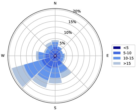
Figure 4.
Wind rose for Seagreen farm site [18]. Colours show the range of wind speed (m/s).
3.5. FLORIS
The software used to run the wind farm simulations and analysis is FLORIS (FLOw Redirection and Induction in Steady State) Version 2.4 [19]. FLORIS is an open-source wind farm optimisation tool developed by the National Renewable Energy Laboratory (NREL). It provides a control-oriented model of steady-state wakes in a wind farm. FLORIS is capable of using several different wake models; the wake model chosen for this study is a Gaussian model of Niayifar and Porté-Agel [20]. All models and parameters adopted in FLORIS are summarised in Table 2.
Table 2.
Summary of FLORIS setup.
The incoming wind speed for each rotor () is calculated from a square grid of only 3 × 3 points on each rotor plane (with a uniform spacing of half radius) as the effect of increasing the number of points was found to be negligibly small. For the calculation of the farm-average wind speed (), a rectangular grid of 250 × 160 points (covering the rectangular farm area of 27.0 km × 17.5 km with an approximately uniform spacing of 108 m and 109 m in each direction) was found to be sufficient to obtain grid-independent results. Note that the two-scale momentum theory [9] suggests that, in general, should be calculated from a volume average across a wind farm layer; however, in this study we calculate it from a surface average at the hub-height (to reduce the computational cost). This simplification is justified as this study adopts an empirical wake model (which is unlikely to predict the vertical structure of the wind farm layer accurately) and also ignores the vertical shear of the background wind profile.
3.6. AEP Calculation
The annual energy production (AEP) shows how much power the wind farm produces during a year. The farm power for each combination of wind speed and wind direction, , is calculated first and then multiplied by its corresponding probability from the wind rose, , and all these are summed to get the AEP (in GWh):
where N denotes the number of combinations of wind speed and wind direction. There are a total of 360 combinations with 30 wind speeds (1 to 30 m/s at 1 m/s intervals) and 12 wind directions (0° to 330° at 30° intervals) in this study.
4. Results
4.1. Case 0
This is our ’baseline’ case where the effect of wind extractability is not considered and hence the farm upstream wind speed (or ’inflow’ speed) is not affected by the wind farm (i.e., = in Figure 1). Figure 5 shows the hub-height flow fields predicted using FLORIS for four different wind directions (0°, 120°, 150°, and 240°) with a fixed inflow speed on 11.4 m/s (rated wind speed). At 120°, many turbines are in the wake of upstream turbines, leading to large wake losses at this wind direction, whereas at 150° and 240°, most turbines are misaligned with the wind direction, meaning that the farm power is high at these wind directions. This can be confirmed from Figure 6, which shows how the farm power varies with wind direction. It can be seen that the predicted power loss due to wake losses is more than 30% at 120° and 300°, but less than 20% at the other wind directions (note that the rated capacity of the farm is 1500 MW). As shown earlier in Figure 4, the range of wind directions expected at this site is between 150° and 240° for most of the time, explaining why this turbine layout has been designed to achieve a high farm power at these wind directions.
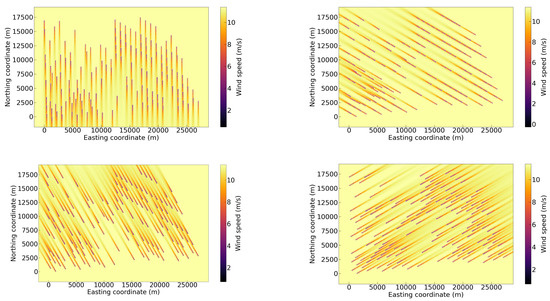
Figure 5.
Snapshots of hub-height flow fields for a fixed inflow speed of = = 11.4 m/s with different wind directions: 0° (upper left), 120° (upper right), 150° (lower left), and 240° (lower right).
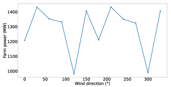
Figure 6.
Variation of farm power with wind direction (for a fixed inflow speed of 11.4 m/s).
The farm power prediction was repeated for all combinations of different wind speeds (from 4 to 25 m/s, at which the turbines generate power) and directions to calculate the AEP, which was found to be 7376 GWh (equivalent to a capacity factor of 56.1%) for Case 0. This will be compared with Cases A and B in the following subsections.
4.2. Case A
Case A builds on Case 0 in the sense that the load control strategy remains the same, but the effects of wind extractability (and thus wind farm blockage losses) are considered. To do this, the two-scale momentum theory described in Section 2 is used to correct the farm-upstream wind speed (from to as in Figure 1).
4.2.1. Correcting Farm-Upstream Wind Speed
The correction of inflow speed is made for each combination of 30 different natural wind speeds () and 12 different wind directions, using the following iterative process. First, the values of () and (Equation (2)) are calculated or ’measured’ using FLORIS. For the first iteration, the inflow speed used in FLORIS is . Secondly, the ’measured’ value of is substituted into the following equation (obtained from Equations (1) and (3) with assuming ) to calculate a ’true’ value of :
This is a quadratic equation which can be solved analytically to obtain for a given set of parameters (, and ). To satisfy the farm-scale momentum balance, the ’measured’ value of obtained from FLORIS needs to agree with the ’true’ value of obtained from Equation (7). To achieve this, we adopt a simple iterative process which continues to update the inflow speed using the following relationship until the difference between the two values becomes less than 0.1%:
Table 3 summarises the number of iterations required for convergence. Only 2 to 3 iterations were found to be sufficient in most cases, although a small number of cases required more iterations (9 iterations at the maximum). Figure 7 shows an example of how the values converge and the error decreases down to less than 0.1% during the iterative process.
Table 3.
Number of iterations required to correct the inflow speed in Case A.
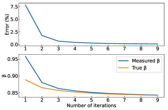
Figure 7.
Variation of the ’measured’ and ’true’ values during the iterative process (for the case that required the largest number of iterations).
4.2.2. Results
Figure 8 shows how () changes with the natural wind speed () once the effect of wind extractability () is taken into account. The initial (or uncorrected) values obtained in Case 0 are also plotted here for comparison. As expected from the two-scale momentum theory, the farm-average wind speed becomes lower when the wind extractability is low, and its impact is larger at lower wind speeds (at which the turbine thrust coefficient is higher). As increases, the differences between the initial (uncorrected) and corrected values of decrease. This means that the farm blockage effect diminishes at higher wind speeds (as the thrust coefficient decreases).
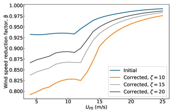
Figure 8.
Comparison of the initial (Case 0) and corrected (Case A) values of for different natural wind speeds (with a fixed wind direction of 0°).
Figure 9 shows how the farm-upstream wind speed and farm-average wind speed change with the wind direction, at a fixed natural wind speed of 10 m/s. It can be seen that the farm-upstream wind speed also depends significantly on the wind extractability; it decreases by about 12% at = 10 but only about 5% at = 20. It also varies with wind direction; for example, wake interactions are significant at 120° and 300° as shown earlier in Figure 6 and hence tends to be lower at these wind directions, resulting in a smaller reduction of farm-upstream wind speed (as well as the farm-average wind speed). However, these results suggest that the effect of wind direction is less significant compared to the effect of wind extractability.
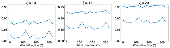
Figure 9.
Wind speed reduction factors in Case A for all wind directions at = 10 m/s. Solid lines show the farm-upstream wind speed reduction factor () and dashed lines show the farm-average wind speed reduction factor ().
Figure 10 shows the variation of farm-average turbine power with natural wind speed, for a fixed wind direction of 0° as a representative example. Results for Case 0 are also plotted for comparison (note that the difference between Case 0 and Case A corresponds to the farm blockage losses). It can be seen that the rated power of 10 MW is still reached by turbines in Case A, but a slightly higher wind speed () than in Case 0 is required due to the farm blockage effect. As expected, the farm blockage losses increase as the wind extractability decreases.
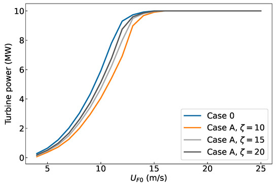
Figure 10.
Comparison of farm-average turbine power between Case 0 and Case A (with a fixed wind direction of 0°).
Finally, the power prediction was repeated for all combinations of wind speeds and directions to calculate the values of AEP for the low, medium and high wind extractability scenarios, which are summarised in Table 4. As expected, the reduction of AEP from Case 0 (i.e., power loss due to wind farm blockage) depends significantly on the wind extractability, varying between 15.4% at = 10 and 5.7% at = 20.
Table 4.
AEP values for Case A.
4.3. Case B
In Case B the effect of wind extractability is considered again as in Case A, but now the turbine operating points are adjusted or re-optimised taking into account the extractability, to reduce the negative impact of farm blockage and hence improve the power production.
4.3.1. Re-Optimising Turbine Operating Conditions
In this study we consider a simple adjustment of blade pitch angle and TSR only in Region 2b of turbine operation. This means that the turbine power coefficient in Region 2b will be lower than that used in Case A, but the turbine thrust coefficient will also be lower, leading to a reduction in and hence an increase in and the overall power production. The reason for focusing on Region 2b is because this wind speed range is low enough for the wind extractability to have a significant impact on but also high enough for the impact of power increase on the AEP to be substantial. Further adjustment of operating points in Regions 2a and 2c may result in some additional power increase, but this is not considered in the present study.
To find the new optimal operating point for Region 2b, first, we find possible combinations of blade pitch angle and TSR for a given value, for example, 90%, 80%, 70%, 60% and 50% of the original value () as shown in Figure 11. Here we applied a two-dimensional linear interpolation to the original and tables to have more data points with smaller intervals of pitch angle and TSR (0.01 instead of 0.25). Secondly, we find the operating point that maximises for a given . As can be seen from Figure 12, there is a single optimal point for a given ; for example, the optimal pitch angle increases from 0.75° to about 7° and the optimal TSR decreases from 8.0 to about 5.7 as the selected value of decreases from to 0.5. Hence, now the question is how to find the optimal level of reduction in .
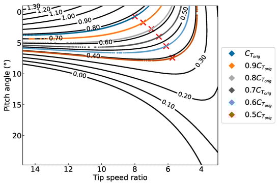
Figure 11.
Contour plot of for the DTU 10 MW turbine. Each coloured line represents possible operating points for a given reduction in for Region 2b (with markers showing the optimal points).
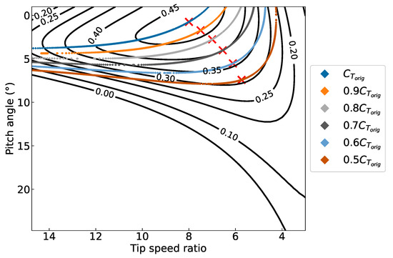
Figure 12.
Contour plot of for the DTU 10 MW turbine, overlaid by the same coloured lines as in Figure 11 showing possible operating points for a given reduction in for Region 2b.
The difficulty in finding the optimal reduction of is that this depends on the wind speed and direction as well as the wind extractability, meaning that a number of FLORIS simulations would be required to find the true optimal point for each wind condition. To reduce the number of FLORIS simulations and the computational cost, here we attempt to find an approximately optimal point using an assumption that is proportional to ; for example, if our trial is 90% of the original value used in Case A, we assume that is also 90% of the value obtained in Case A. This assumption allows us to estimate the value of (by solving Equation (7) for ) and then the farm-upstream wind speed from the following equation without running FLORIS simulations:
The above calculation of , and then a single FLORIS simulation using the calculated value, are performed for a range of trial values (between 1.0 and 0.5) to find the (approximately) optimal reduction of , for each of the 12 different wind directions (but only at = 10 m/s as a representative wind speed for Region 2b). This reduces the computational cost required to find a new optimal operating point for Region 2b (as otherwise we would need a handful of iterations of FLORIS simulations to obtain the correct , and values as we did in Case A, for each trial case). Note, however, that the above assumption/approximation is used only in the process of finding this new optimal operating point. The final AEP calculation for Case B is conducted using the same iterative process as in Case A.
Although the present re-optimisation method focuses on the adjustment of operating conditions only in Region 2b, we also adjust the upper-end wind speed for Region 2b. This adjustment is required as the turbine rotational speed should be at the maximum possible value in Region 2c (10 rpm) and the turbine power should be at the rated value in Region 3 (10 MW). Since TSR decreases as we reduce in Region 2b, the maximum rotational speed is reached at a higher value, increasing the upper-end wind speed for Region 2b. Similarly, since decreases as we reduce , the rated power may also be reached at a higher than the original rated wind speed (if the reduction of in Region 2b is large enough to eliminate Region 2c). Figure 13 and Figure 14 show some examples of how the and curves are adjusted depending on different levels of reduction in Region 2b. It can be seen that the rated wind speed increases from the original value of 11.4 m/s to a higher value when in Region 2b is reduced to less than about 80% of the original value.
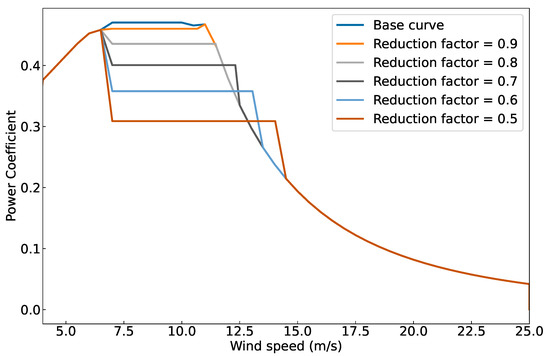
Figure 13.
curves obtained for different levels of thrust reduction, compared against the base curve used in Case 0 and Case A.
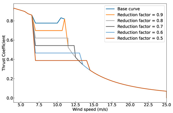
Figure 14.
curves obtained for different levels of thrust reduction, compared against the base curve used in Case 0 and Case A.
4.3.2. Results
Figure 15 shows how the wind farm power at = 10 m/s changes as we reduce the value of from 1.0 to 0.5 , for the low ( = 10) and high ( = 20) extractability scenarios. Note that here the farm power has been normalised by the corresponding farm power obtained in Case A, for each of 12 different wind directions. It can be seen that the optimal reduction of is about 0.8 and 0.85 (depending on wind direction) at = 10, and about 0.9 at = 20. The maximum increase in the farm power (compared to Case A) is about 3.5% to 4.5% at = 10 (depending on wind direction) and about 1.5% at = 20. As expected, the farm power becomes lower than Case A if we reduce too much.
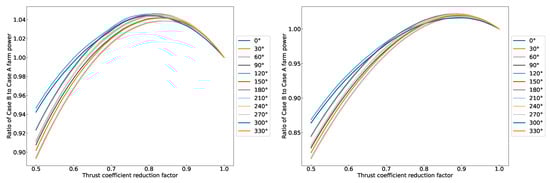
Figure 15.
Impact of reduction on the wind farm power (relative to Case A) at 12 different wind directions with a fixed natural wind speed of = 10 m/s, for two different wind extractability scenarios: = 10 (left) and 20 (right).
Figure 16 compares the farm-upstream wind speed reduction factor () between Case A and Case B (adopting the optimal reduction at each wind direction) at = 10 m/s. It can be seen that the is higher in Case B than in Case A due to the reduced turbine thrust. The dependency of on wind direction is similar between Case A and Case B, whilst the impact of wind extractability is still significant.
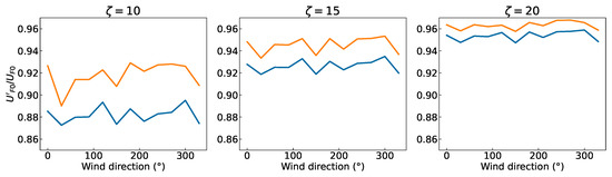
Figure 16.
Farm-upstream wind speed reduction factor for all wind directions at = 10 m/s, for Case A (blue) and Case B (orange).
Finally, the AEP values calculated for Case B are summarised in Table 5 for the three different extractability scenarios. The improvement of AEP from Case A (i.e., improvement due to the mitigation of farm blockage losses) depends on the wind extractability, varying between 2.0% at = 10 and 0.6% at = 20. These improvements are smaller than the improvements shown earlier for a fixed wind speed of = 10 m/s (Figure 15) but still promising, considering the simplicity of the mitigation method used in this study.
Table 5.
AEP values for Case B.
5. Discussion and Conclusions
In this study we have demonstrated a new method to predict the power losses due to wind farm blockage and how they could be mitigated by re-optimising turbine operating points, for a realistic large wind farm (resembling the Seagreen offshore wind farm [18]) off the east coast of Scotland. The new method, which was derived from the two-scale momentum theory of Nishino and Dunstan [9,13], is relatively simple and can be applied to existing engineering wind farm models easily with small additional computational cost.
The main source of uncertainty of the new method lies in the assessment of the wind extractability factor () using an NWP model [12]. The predicted farm blockage losses (for the case without re-optimising turbine operating points) vary significantly from about 5% for a high extractability scenario ( = 20) up to about 15% for a low extractability scenario ( = 10). A recent study [13] suggests that the extractability factor tends to decrease as the wind farm size increases. Further investigations will be required in future studies to better predict the wind extractability factor.
Nevertheless, the present study suggests that the optimal reduction of required to maximise the farm power is not very sensitive to the wind extractability factor (for an expected typical range of ) or the wind direction (Figure 15). This implies that a simple adjustment of blade pitch angle and TSR used below the rated wind speed (at which the farm blockage effect is most significant) may be sufficient to increase the AEP of existing large offshore wind farms. Our results show that even a highly simplified re-optimisation process (which requires less computational cost to find the new optimal operating points compared to a more sophisticated process) may increase the AEP by about 0.6% to 2.0% depending on the wind extractability.
In this study we did not use any turbine induction models (such as [10,11]) to predict the wind farm blockage effect. These induction models could be used together with the present method, and in that case, it is expected that Equation (7) would still act to correct the farm-average wind speed reduction factor (and then the farm-upstream wind speed ) such that the farm-scale momentum balance is approximately satisfied for a given . Finally, it should also be noted that a full validation of the proposed approach (through a direct comparison with real wind farm data) is currently infeasible as this would require time series of ‘in-situ’ wind conditions for two scenarios in parallel (i.e., one with and one without the wind farm).
Author Contributions
Conceptualization, T.N.; methodology, L.L., T.N. and E.P.-C.; software, L.L., M.L.P. and E.P.-C.; analysis, L.L., M.L.P. and T.N.; writing—original draft preparation, L.L.; writing—review and editing, T.N.; supervision, T.N. and E.P.-C. All authors have read and agreed to the published version of the manuscript.
Funding
This research received no external funding.
Institutional Review Board Statement
Not applicable.
Data Availability Statement
The data presented in this paper are available on request from the corresponding author.
Acknowledgments
We thank Mark Faber and Andrew Kirby for helpful discussion and assistance with the analysis of computational results.
Conflicts of Interest
The authors declare no conflict of interest.
Abbreviations
The following abbreviations are used in this manuscript:
| ABL | Atmospheric boundary layer |
| AEP | Annual energy production |
| CV | Control volume |
| NDFM | Non-dimensional farm momentum |
| NWP | Numerical weather prediction |
| TSR | Tip-speed ratio |
References
- Department for Business, Energy and Industrial Strategy (BEIS). Energy Trends UK, October to December 2020 and 2021; Department for Business, Energy and Industrial Strategy (BEIS) of the Government of the UK: London, UK, 2022.
- Howland, M.F.; Lele, S.K.; Dabiri, J.O. Wind farm power optimization through wake steering. Proc. Natl. Acad. Sci. USA 2019, 116, 14495–14500. [Google Scholar] [CrossRef] [PubMed]
- Munters, W.; Meyers, J. Towards practical dynamic induction control of wind farms: Analysis of optimally controlled wind-farm boundary layers and sinusoidal induction control of first-row turbines. Wind Energy Sci. 2018, 3, 409–425. [Google Scholar] [CrossRef]
- Frederik, J.A.; Weber, R.; Cacciola, S.; Campagnolo, F.; Croce, A.; Bottasso, C.; van Wingerden, J.-W. Periodic dynamic induction control of wind farms: Proving the potential in simulations and wind tunnel experiments. Wind Energy Sci. 2020, 5, 245–257. [Google Scholar] [CrossRef]
- Zhang, M.; Arendshorst, M.G.; Stevens, R.J.A.M. Large eddy simulations of the effect of vertical staggering in large wind farms. Wind Energy 2019, 22, 189–204. [Google Scholar] [CrossRef]
- Chatterjee, T.; Peet, Y. Exploring the benefits of vertically staggered wind farms: Understanding the power generation mechanisms of turbines operating at different scales. Wind Energy 2019, 22, 283–301. [Google Scholar] [CrossRef]
- Meyers, J.; Bottasso, C.; Dykes, K.; Fleming, P.; Gebraad, P.; Giebel, G.; Göçmen, T.; van Wingerden, J.-W. Wind farm flow control: Prospects and challenges. Wind Energy Sci. 2022, 7, 2271–2306. [Google Scholar] [CrossRef]
- Bleeg, J.; Purcell, M.; Ruisi, R.; Traiger, E. Wind farm blockage and the consequences of neglecting its impact on energy production. Energies 2018, 11, 1609. [Google Scholar] [CrossRef]
- Nishino, T.; Dunstan, T.D. Two-scale momentum theory for time-dependent modelling of large wind farms. J. Fluid Mech. 2020, 894, A2. [Google Scholar] [CrossRef]
- Branlard, E.; Meyer Forsting, A.R. Assessing the blockage effect of wind turbines and wind farms using an analytical vortex model. Wind Energy 2020, 23, 2068–2086. [Google Scholar] [CrossRef]
- Segalini, A. An analytical model of wind-farm blockage. J. Renew. Sustain. Energy 2021, 13, 033307. [Google Scholar] [CrossRef]
- Patel, K.; Dunstan, T.D.; Nishino, T. Time-dependent upper limits to the performance of large wind farms due to mesoscale atmospheric response. Energies 2021, 14, 6437. [Google Scholar] [CrossRef]
- Kirby, A.; Nishino, T.; Dunstan, T.D. Two-scale interaction of wake and blockage effects in large wind farms. J. Fluid Mech. 2022, 953, A39. [Google Scholar] [CrossRef]
- Lanzilao, L.; Meyers, J. Set-point optimization in wind farms to mitigate effects of flow blockage induced by atmospheric gravity waves. Wind Energy Sci. 2021, 6, 247–271. [Google Scholar] [CrossRef]
- Allaerts, D.; Meyers, J. Sensitivity and feedback of wind-farm-induced gravity waves. J. Fluid Mech. 2019, 862, 990–1028. [Google Scholar] [CrossRef] [PubMed]
- HAWC2. DTU 10-MW Reference Wind Turbine. Available online: https://www.hawc2.dk/Download/HAWC2-Model/DTU-10-MW-Reference-Wind-Turbine (accessed on 25 March 2022).
- GitHub. Cp-Ct-Cq Table for Control. Available online: https://github.com/Seager1989/DTU10MW_FAST_LIN/blob/main/Cp_Ct_Cq.DTU10MW.txt (accessed on 25 March 2022).
- Marine Scotland. Seagreen Offshore Wind Farm. Available online: https://marine.gov.scot/sites/default/files/owf_dslp.pdf (accessed on 26 March 2022).
- NREL. FLORIS: FLOw Redirection and Induction in Steady State. Available online: https://www.nrel.gov/wind/floris.html (accessed on 26 March 2022).
- Niayifar, A.; Porté-Agel, F. Analytical modeling of wind farms: A new approach for power prediction. Energies 2016, 9, 741. [Google Scholar] [CrossRef]
- Crespo, A.; Hernandez, J. Turbulence characteristics in wind-turbine wakes. J. Wind Eng. Ind. Aerodyn. 1996, 61, 71–85. [Google Scholar] [CrossRef]


Disclaimer/Publisher’s Note: The statements, opinions and data contained in all publications are solely those of the individual author(s) and contributor(s) and not of MDPI and/or the editor(s). MDPI and/or the editor(s) disclaim responsibility for any injury to people or property resulting from any ideas, methods, instructions or products referred to in the content. |
© 2022 by the authors. Licensee MDPI, Basel, Switzerland. This article is an open access article distributed under the terms and conditions of the Creative Commons Attribution (CC BY) license (https://creativecommons.org/licenses/by/4.0/).