Exploring the Relationship between Crude Oil Prices and Renewable Energy Production: Evidence from the USA

Abstract

This study aims to examine the short-term and long-term relationship between WTI oil prices and renewable energy production considering U.S. crude oil production, world oil prices, and other domestic and global factors. We employ several time-series analysis techniques, including the augmented Dickey-Fuller test and the Phillips-Perron test for unit roots; the long-term relationship is examined using fully modified OLS (FMOLS) and Park’s canonical cointegration regression (CCR). We also utilise an error correction model (ECM) to distinguish between short- and long-term effects. It is shown that at a constant level of crude oil production, an increase in energy production from renewable sources is accompanied by an increase in oil prices. Thus, at this stage of development, despite the increased production, renewable energy can be considered as complement to but not a substitute for crude oil. Our empirical estimations allow us to conclude that renewable energy production today is pushing the price of oil up rather than lowering it.

1. Introduction

According to the Statistical Review of World Energy 2022 [1], crude oil production in the United States has steadily increased since 2017, reaching 711.1 million tonnes (Mt) in 2021. As a result, the United States is now one of the world’s top crude oil producers. The Russian Federation and Saudi Arabia are the world’s next largest crude oil producers, with 536.4 Mt and 515 Mt, respectively. In terms of crude oil exports, Saudi Arabia dominated the market in 2021, exporting 323.2 Mt, followed by the Russian Federation with 263.6 Mt, Canada with 197.4 Mt, Iraq with 176.1 Mt, the United Arab Emirates with 146.1 Mt, and the United States with 138.5 Mt, which ranked sixth. The United States has changed its crude oil import and export structure due to the implementation of restrictions on heavy crude oil imports from Venezuela. As a result, the country now exports light oil and imports heavy oil [2].

Despite its domestic production, the United States still relies heavily on crude oil imports to fuel its economy, and this trend is likely to continue for the foreseeable future. Based on the B.P. Statistical Review of World Energy 2022 [1], the United States heavily relied on Canada, South and Central America, and Mexico for its heavy crude oil imports in 2021, from which it imported 187.1 Mt, 29.2 Mt, and 29.0 Mt, respectively. On the other hand, most of the U.S.’s light crude oil imports in 2021 came from Saudi Arabia, amounting to 17.7 Mt. In terms of lighter crude oil imports, the United States had significant trade movements in 2021 with Europe, Canada, South and Central America, India, China, and other Asia Pacific countries, with 51.4 Mt, 15.5 Mt, 8.3 Mt, 20.5 Mt, 11.5 Mt, and 25.1 Mt, respectively. These statistics illustrate the importance of international trade in meeting the United States’ energy demands, with a diverse range of countries supplying crude oil to the nation.

As of 2021, the United States has secured its position as the global front-runner in natural gas production, producing a staggering 934.2 billion cubic meters (Bcm) of this valuable resource. Russia closely trails behind in second place, with a production output of 701.7 Bcm. Iran ranks third with 256.7 Bcm, followed by China in fourth place with 209.2 Bcm. Regarding natural gas exports, the United States shipped out 179.3 Bcm in 2021, while Russia exported 241.3 Bcm. It is noteworthy that these statistics highlight the United States’ dominance in the global natural gas market, as they produce the most while still managing to export a significant portion of their resources to other countries [1].

Given that the United States is the largest producer of crude oil globally and holds considerable sway over energy prices, our model’s selection of the WTI price as the dependent variable was appropriate. To this end, our model must incorporate data on the production and consumption of crude oil in the United States.

The prices of WTI crude oil in the United States significantly impact the global economy and financial markets. Therefore, investigating and modelling the prices of WTI crude oil is a crucial direction for economic and financial analysis. WTI crude oil plays a vital role in the U.S. economy and international trade, meaning that even slight changes in oil prices can considerably impact the global economy. The cost of WTI crude oil directly affects the prices of gasoline, diesel fuel, and other oil products, which, in turn, influences the expenses of consumers and businesses. Furthermore, fluctuations in WTI crude oil prices can also affect inflation, currency exchange rates, and even political stability in regions that rely on the oil industry. Thus, analysing WTI crude oil prices can help businesses and investors make more informed decisions in their operations, and it can assist governments in developing more effective political and economic strategies amidst the uncertainty in the oil market.

The OPEC oil price is a critical factor influencing the global oil market. This price is determined by the balance of supply and demand for oil, which in turn depends on various factors such as economic growth, political instability, changes in production, and technological innovations. The OPEC oil price also affects the price of WTI oil, as they are closely linked to each other. However, it should not be forgotten that the markup for WTI oil also depends on other factors, such as crude oil types such as Brent and Dubai Crude. This effect is attributed to the high cost of crude oil extraction using the U.S. Hydraulic fracturing technology. As global crude oil prices increase, hydraulic fracturing becomes more lucrative. The Drilling Productivity Report [3] notes that an increase in the number of active wells in the U.S. leads to increased oil production. However, drilling new wells generally costs more than fracturing existing ones and enhancing their productivity. The U.S. fracking boom [4] has resulted in a surge in crude oil production and increased global supply, driving down world oil prices. The reduction in world oil prices triggers the closure of unprofitable wells and a decrease in oil production in the U.S., which directly impacts the WTI price formation and can be incorporated into the model.

However, it also highlights the significance of renewable energy sources as a potential solution to reduce dependence on fossil fuels. With the rise of renewable energy, such as solar and wind power, the demand for crude oil may decrease, thus leading to a reduction in hydraulic fracturing and crude oil production. Moreover, as renewable energy technologies continue to advance and become more affordable, they could become more competitive with traditional energy sources. This could result in a shift towards renewable energy sources and a decrease in the use of fossil fuels, which would not only reduce the impact on the environment but also provide long-term economic benefits. Therefore, the insights gained from understanding the dynamics of crude oil production can inform the transition towards a more sustainable energy future.

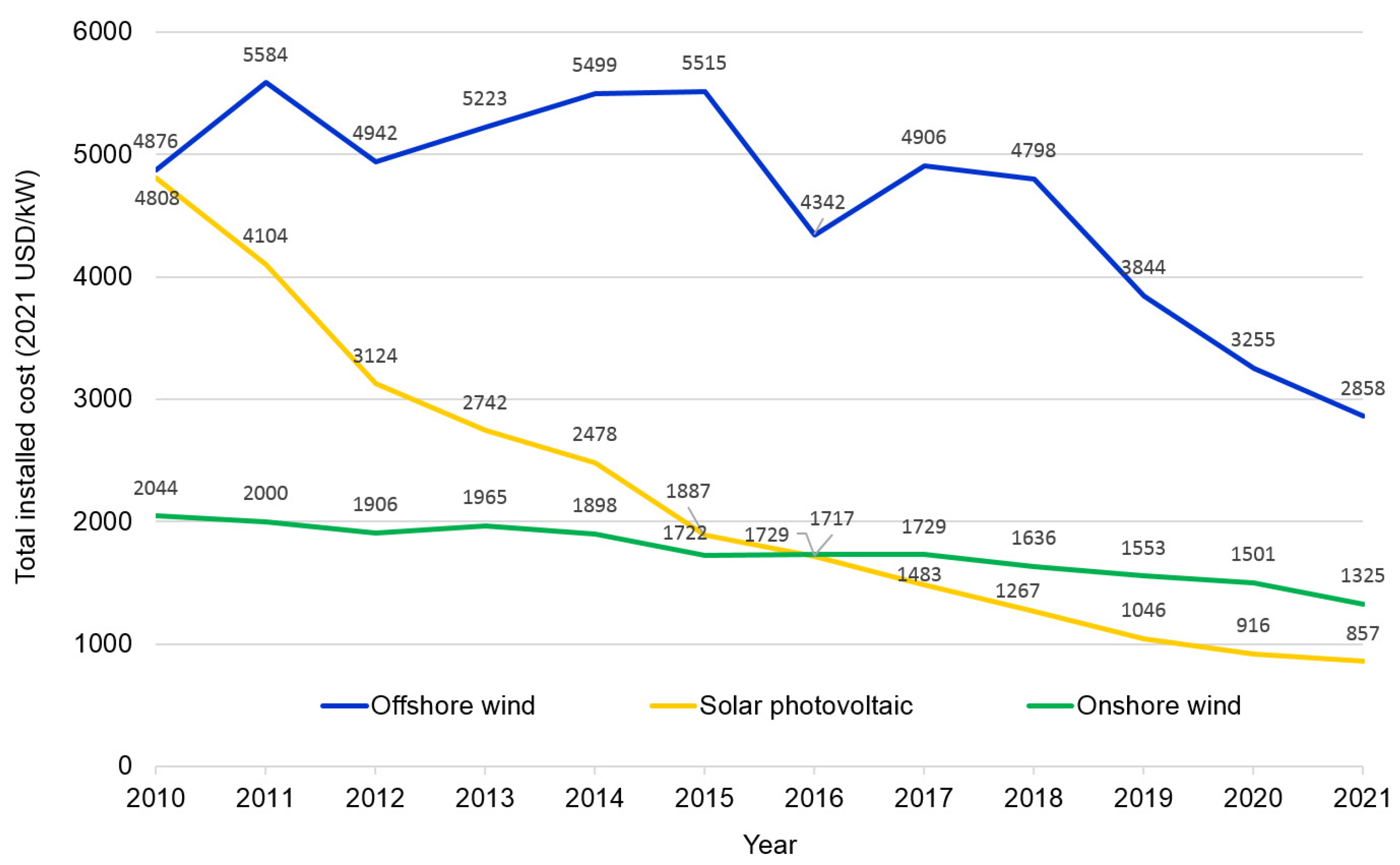
Based on the report on renewable power generation costs by the International Renewable Energy Agency [5], it has been observed that there has been a significant decline in the global weighted-average total installed cost of onshore wind farms, offshore wind farms, and solar photovoltaic installations over the past decade. Specifically, the total installed cost of onshore wind farms has decreased from USD 2044/kW in 2010 to USD 1325/kW in 2021, indicating a decline of 1.54 times. Similarly, the total installed cost of offshore wind farms has reduced from USD 4876/kW in 2010 to USD 2858/kW in 2021, showing a decline of 1.71 times. Moreover, solar photovoltaic installations have experienced the most significant decline in total installed costs, with the cost decreasing from USD 4808/kW in 2010 to USD 857/kW in 2021, indicating a decline of 5.61 times. These cost reductions signify the growing affordability and accessibility of renewable energy sources, which could pave the way for a cleaner and more sustainable energy future for the world (Figure 1).

Solar power has come a long way since its inception in space exploration, and its adoption has grown in recent years. Despite initial costs and challenges associated with using solar panels on Earth, advancements in technology and mass production have made solar power more accessible and affordable. Solar panels can now harness energy even in cloudy or low-light conditions, making them a viable option for renewable energy. Additionally, solar power is eco-friendly and can reduce our carbon footprint, making it a prime example of sustainable energy that can play a pivotal role in mitigating the impacts of climate change. As we strive towards a cleaner and more sustainable future, solar power has immense potential to become a reliable and uninterrupted renewable energy source.

Solar photovoltaic (P.V.) technology’s production costs have significantly declined over the past few decades. According to studies conducted between 1976 and 2019, the cost of generating electricity through solar panels has reduced considerably from $106 to $0.38 per 1 watt generated. This decrease in the cost of 278 times is a significant milestone in the solar energy industry. This cost reduction is attributed to various factors such as technological advancements, economies of scale, and increased investment in research and development. As the solar energy sector continues to grow, it is expected that the cost of producing electricity generated by solar P.V. technology will continue to decrease further, making it a more affordable and accessible source of energy for consumers worldwide [5]. This is seen on a logarithmic scale; the solar photovoltaic and onshore wind data are almost linearised in Figure 2. In their work, Lafon et al. (2017) showed that for solar photovoltaic cell/module systems, the rate of cost reduction as the electricity they produced doubled was 20.2% (Figure 2) [6].

In 2020–2021, renewable energy production through solar photovoltaic and onshore wind sources reached a significant milestone by breaking through the bottom of prices. As a result, they have become more affordable energy sources than new projects based on fossil fuels. The pricing of these renewable sources has remained competitive, even amidst rising oil and gas prices, especially in the year 2022. This has significantly increased the competitive advantages of solar P.V. and onshore wind technology, making them even more desirable energy sources for commercial and residential use.

Numerous factors contribute to the forecasting of oil prices. These factors can be categorised into various areas, such as politics, economics, the environment, and sanctions restrictions. All these factors must be considered to ensure compliance with the supply-demand balance. It is important to note that the equilibrium oil prices can vary considerably depending on the specific scenario being considered. As such, it is crucial to consider all the factors that could influence the price of oil when attempting to forecast future prices. By doing so, we can better understand the future of this critical commodity.

Consider four possible scenarios out of a vast array of potential outcomes. The International Energy Agency (IEA) scenarios [8] have predicted the following oil prices by 2050, namely STEPS (Stated Policies Scenario), APS (Announced Pledges Scenario), and NZE (Net Zero Emissions by 2050 Scenario), which forecast the oil prices to be 95 USD per barrel, 60 USD per barrel, and 24 USD per barrel, respectively, by the year 2050 (based on 2021 prices). Meanwhile, the U.S. Energy Information Administration (EIA) has predicted the highest oil price by 2050 through its High Oil Price scenario, which corresponds to 175 USD per barrel (based on 2020 prices) [9]. On the other hand, forecasting energy prices in the European Union is even more daunting because of the significant fluctuations observed in the historical period due to the considerable supply shortage in the market.

The available long-term forecast options for the maximum and minimum oil prices up to the year 2050 exhibit significant variations. However, it is essential to note that these predictions do not necessarily dictate the exact trajectory of the long-term price of oil. We understand that the specified range allows for price spikes to occur within certain conditions and at specific times. Hence, while these forecasts provide valuable insight into potential future trends, they are subject to numerous factors that may cause fluctuations in oil prices. As such, it is essential to remain vigilant and adaptable to unexpected changes.

This investigation aims to analyse the connection between WTI oil prices and U.S. crude oil production, both in the short term and long term. To achieve this goal, we consider various factors, such as global oil prices, national natural gas prices, and renewable energy output. We apply numerous time series analysis methods, such as the Augmented Dickey-Fuller test and the Phillips-Perron test for unit roots, and the fully modified OLS (FMOLS) and Park’s canonical cointegration regression (CCR) to examine the long-term relationship. This article contributes to the crude oil literature in a number of important ways. First, the cointegration approach used in this article directly shows a cointegrating relationship between WTI prices, U.S. crude oil production, OPEC oil prices, and renewable energy production. Furthermore, we employ an error correction model (ECM) to differentiate between short- and long-term effects. Our findings demonstrate that when crude oil production remains constant, a rise in renewable energy production is associated with an increase in oil prices. Consequently, despite the growth in renewable energy production, it is still regarded as a complementary energy source rather than a substitute for crude oil at this stage of development.

The structure of our paper is as follows: In Section 2, we provide a comprehensive literature review of the relevant scientific field. Our methodology is presented in Section 3, while Section 4 details our empirical findings. Section 5 and Section 6 then delve into discussions and conclusions drawn from our research.

2. Literature Review

The oil and gas industry has been the backbone of global energy production for many decades, with the United States being one of the leading crude oil producers. However, with the increasing concerns over the environmental impact of fossil fuels and the push towards renewable energy sources, the energy market dynamics have been shifting rapidly. This has led to a renewed interest in understanding the impact of various factors, such as crude oil production, global oil prices, renewable energy production, and clean energy company returns on WTI futures prices. Different empirical studies have investigated the current state of knowledge in this area. By doing so ourselves, we aim to contribute to a better understanding of the complex interactions between different factors in the energy market and their influence.

Dimitriadis, D. and Katrakilidis, C.’s research [10] investigates the ever-changing relationships between the market prices of ethanol, crude oil, and corn in the United States between January 2005 and December 2014. To ensure the robustness of the empirical analysis, various time series methodologies were employed, including the single equation and system estimation approaches to cointegration. Specifically, the autoregressive distributed lags and the Johansen cointegration methodologies were applied complementarily. The research findings show a statistically significant long-term causal effect that flows from both crude oil and corn prices to ethanol prices and from ethanol and corn prices to crude oil prices. Moreover, a positive correlation between crude oil prices and ethanol was uncovered.

Another paper [11] presents the first-ever analysis of the asymmetric response of petroleum product prices to international crude oil prices in Nigeria. The study uses the hidden cointegration approach on quarterly data from 1973Q1 to 2020Q2. After conducting preliminary tests of data description, unit root analysis, and a cointegration test, the study reveals that positive and negative components of both crude oil and petroleum prices move together in the long term. The empirical findings from both the long-term and short-term results indicate that petroleum prices in Nigeria respond asymmetrically to changes in crude oil prices. Specifically, the study found that positive changes (increase) in crude oil prices have a larger and stronger effect on petroleum prices than the effect of negative changes (decrease) in crude oil prices.

The next study explores the changing connection between oil prices and stock prices in African markets over time. The authors utilised a wavelet-based dynamic conditional correlation framework, which enabled them to examine the time-varying correlation between oil prices and African stock markets across different time and frequency domains. Empirical findings indicate that the interdependence between these two markets varies over time and is spread out across different wavelet scales. The dynamic relationship between oil prices and stock returns in these countries was discovered to be more variable in the short term, occurring more frequently and at a lower level. Long- and medium-term co-movements exist between the two markets, except during the COVID-19 pandemic, when short-term integration increased considerably [12].

Rehman et al. [13] examine the nonlinear relationship between oil prices, inflation, and residential prices in the U.S., the U.K., and Canada using quarterly data from 1975 to 2017. The researchers employed the nonlinear autoregressive distributed lag (NARDL) bounds testing approach to explore potential short-term and long-term asymmetric effects. The findings reveal that the relationships between oil prices, interest rates, inflation rates, income, and residential prices in the U.S., U.K., and Canada are asymmetric, albeit to varying degrees. In all three economies, inflation rates have a significant long-term impact on residential prices, while the asymmetric impact of international oil prices is more pronounced in the U.S. than in the U.K. and Canada. Additionally, a long-term asymmetric relationship between residential prices, inflation, and GDP per capita is observed in the U.S., whereas interest rates appear to impact residential prices in both the U.K. and Canada.

Mohanty et al. [14] explore the uneven effects of daily fluctuations in oil prices on various aspects of the U.S. oil and gas industry, including equity returns, market, oil betas, return variances, and trading volumes. Their research indicates that oil and gas firms’ return, market betas, oil betas, and return variances react asymmetrically to changes in oil prices. They discovered that negative changes in oil prices had a more pronounced impact on stock returns than positive changes. Furthermore, decreases in oil prices had a more significant influence on market beta and stock risk than increases in oil prices. Conversely, oil betas and return variances were more affected by oil price increases than decreases.

Samour and Pata [15] explore how the U.S. interest rate and oil prices affect renewable energy usage in Turkey through spillover effects. Using a new method called bootstrap autoregressive distributed lag analysis, the researchers examine annual data from 1985 to 2016, making this the first study in the energy economics literature. The study reveals that the U.S. interest rate has a significant spillover effect on renewable energy use in Turkey, impacting it through income and local interest rate channels. Given Turkey’s limited foreign exchange reserves, high foreign debt, low international reserves, and local currency devaluation, the Turkish economy is closely linked to the U.S. economy through international trade and investment. These factors make the spillover effect of the U.S. interest rate on energy consumption in Turkey even stronger. Furthermore, the study shows that the price of oil harms renewable energy use through the natural income channel.

Han et al. [16] aimed to examine the transmission and feedback mechanisms between international crude oil prices and China’s refined oil prices from January 2011 to November 2015 using various statistical methods such as the Granger causality test, vector autoregression model, impulse response function, and variance decomposition methods. The results show that changes in international crude oil prices can cause a weak feedback effect on China’s domestic refined oil price. Additionally, the lag in international crude oil prices and China’s domestic refined oil prices affect each other to varying degrees, both positively and negatively. An international crude oil price shock has a significant positive impact on domestic refined oil prices, but the impulse response of the international crude oil price variable to the domestic refined oil price shock is insignificantly negative. Moreover, a solid historical inheritance exists between international crude oil prices and domestic refined oil prices.

The study of Balashova and Serletis shows that oil price volatility, estimated using the GARCH-M(1,1) model, constrains TFP growth in both “old” and “new” EU countries, slowing down the pace of innovation and investment activity [17].

Jiranyakul Komain investigates the impact of crude oil prices on inflation in ten countries in Asia and the Pacific countries, all dependent on oil imports. The time frame of analysis spans from May 1987 to December 2019. The findings of the bounds testing for cointegration reveal that, for the most part, there is a stable positive long-term correlation between crude oil prices and the consumer price index in these countries during periods of low and less volatile oil prices. In the long term, the extent to which crude oil prices pass through to consumer prices is only partial. In the short term, there is a weak relationship between crude oil price fluctuations and inflation in most cases, but this pass-through effect is more significant during times of high and more unstable oil prices. Therefore, a structural break appears to be significant in the long- and short-term pass-through effects of crude oil prices on consumer prices [18].

The following paper [19] examines the impact of various oil extraction techniques, including horizontal drilling, fracking, and directional drilling, which combines vertical and horizontal drilling, on the behaviour of WTI crude oil prices. The study contributes a fresh perspective to the existing literature on the relationship between oil prices and extraction methods. The analysis employs statistical tools, specifically the VAR model of fractional cointegration, which detects evidence of cointegration between the series, signifying a long-term equilibrium relationship. Additionally, the wavelet transform is used to analyse the structural changes in the WTI oil price that result from modifications in drilling technology. It is indicated that all three extraction methods have a strong correlation with WTI crude oil prices, with the highest levels of correlation. Thus, a decline in crude oil production from the three extraction methods increases crude oil prices. According to Wu and Zhang [20], the global market for crude oil has seen its fair share of volatility, with price fluctuations being influenced by various factors. One of the primary drivers of these changes is political and financial decision-making. Zhang et al. [21] added that geopolitical instability significantly shapes crude oil prices in international markets. It is essential to note that crude oil’s production and consumption directly impact refined oil prices in local markets, as mentioned by Han et al. [16]. This effect is especially significant for the world’s leading economies, including the United States, China, and the Eurozone. Global events, such as changes in the supply of crude oil, shifts in demand, and geopolitical tensions, can influence refined oil prices in these economies. Therefore, policymakers and businesses in these countries must pay close attention to global market trends and geopolitical developments. They should develop strategies to manage risks associated with fluctuations in crude oil prices to ensure economic stability and growth. Such measures may include diversifying energy sources, investing in renewable energy technologies, and developing efficient transportation systems to reduce dependency on fossil fuels. By doing so, they can protect their economies from the negative impacts of fluctuations in crude oil prices and promote sustainable development for future generations.

The importance of studying the relationship of fossil fuel prices with a number of macroeconomic factors is due to the fact that inflation is largely shaped by energy carriers and, specifically, by fuel price [22]. Another paper analysed methods of forecasting energy consumption and classified more than two hundred approaches to the analysis of the energy market [23,24]. Przekota’s paper [25] created a VAR model to study the Polish economy which considered several factors such as fuel prices, seaborne trade, gross domestic product, and inflation. The findings suggest that the Polish economy can withstand market instability in the fuel industry and a country’s development does not rely solely on low fuel prices. A nation’s economy can grow, even with high fuel prices, and panicking over elevated fuel costs may ignite the inflationary spiral. Such a wide range of research in this field indicates the importance of current scientific work on this topic.

3. Methodology

This paper’s methodology is based on the critical topic of time series analysis, a statistical technique for analysing and modelling time-dependent data.

Our basic econometric model is a linear regression model:

$$y_t=x_t^{\prime }\beta +{\epsilon }_t$$

(1)

where $y_t$ is the dependent variable, $x_t^{}$ is a vector of explanatory variables observed at time $t$, $\beta$ is a vector of parameters, and ${\epsilon }_t$ is a disturbance term.

When working with time series, it is necessary to test their properties, namely whether a series is stationary or not before using it in a regression. Two commonly employed tests for this purpose are the augmented Dickey-Fuller [26] test and the Phillips-Perron test [27], which test the null hypothesis of a unit root. If the null hypothesis is not rejected, a series is nonstationary. A difference stationary series is said to be integrated and is denoted as I(d), where d is the order of integration. Knowing the order of integration is essential for choosing the appropriate technique for estimating equation parameters (1).

If all variables in the equation are of type I (1), Equation (1) is spurious and will produce misleading results. A model in differences can be utilised and estimated using ordinary least squares (OLS):

$${\Delta y}_t={\Delta x}_t^{\prime }\gamma +{\Delta \epsilon }_t$$

(2)

However, what we obtain from Equation (2) is only the short-term relationship between variables.

If we assume that the long-term relationship between the variables exists, then there is a linear combination (a cointegrating equation in form (1)) with a cointegrating vector of weights characterising the long-term relationship between variables. The cointegration method developed by Engle and Granger [28] facilitates the analysis of non-stationary time series.

This paper uses the Engle-Granger residual-based test for cointegration, which is simply a unit root test applied to the residuals obtained from the OLS estimation of Equation (1). A test of the null hypothesis of no cointegration against the alternative of cointegration corresponds to a unit root test of the null of nonstationarity against the alternative of stationarity.

It is well known that if the series are cointegrated, OLS estimation of cointegrating vector $\beta$ in Equation (1) is consistent, converging at a faster rate than is standard, and thus has some important shortcomings [29]. In this case, the fully modified OLS (FMOLS) estimator, developed by Phillips and Hansen [30], can be used to estimate a single cointegration equation. The FMOLS estimator is asymptotically unbiased and eliminates problems caused by the long-term correlation between the cointegrating equation and stochastic regressors innovations.

Another technique for removing long-term dependence is Park’s [31] canonical cointegrating regression (CCR), which is closely related to FMOLS but employs stationary data transformations to eliminate the endogeneity and correct for the asymptotic bias.

An error correction model (ECM) is a popular approach for data where underlying variables have a long-term common stochastic trend, i.e., when the variables are cointegrated. ECMs are theoretically driven, and they help estimate both short-term and long-term effects of one-time series on another.

The term “error correction” in ECM relates to the last period’s deviation from a long-term equilibrium (the error) and influences its short-term dynamics. Thus, ECMs directly estimate the speed at which a dependent variable returns to equilibrium after a change in other variables. In summary, these techniques provide various options for analysing time series data and offer valuable insights into how these series are interconnected and interact over time.

ECM is a reparameterisation of the ARDL model and can be written in the form

$${\Delta y}_t={\Delta x}_t^{\prime }{\gamma }_0+\pi \left[y_{t-1}-x_{t-1}^{\prime }\beta \right]+u_t$$

(3)

In this form, we have an equilibrium relationship ${\Delta y}_t={\Delta x}_t^{\prime }{\gamma }_0+u_t$ and the equilibrium error $\pi \left[y_{t-1}-x_{t-1}^{\prime }\beta \right]$. The coefficient $\pi$ provides the speed of adjustment in case of disequilibrium caused by shocks (captured in the model by error term $u_t$). The coefficient $\pi$ must be negative to boost ${\Delta y}_t$ back to its long-term path as determined by regressors x in Equation (1). All the terms in model (3) are stationary, and standard OLS is valid.

Data Descriptions

Our model utilises a dataset from January 2014 to December 2022, with data collected monthly. The U.S. Production of Crude Oil and Rotary Rigs in Operation was updated in March 2023. This timeframe provides a comprehensive view of the factors under consideration and enables us to generate reliable insights into the studied phenomenon. All relevant information about the factors that make up our model can be found in

Table 1. A priory set of the model variables.

Abbreviated Name	Description	Dimension	Source
WTI	Crude Oil WTI Futures	USD/Bbl	[32]
TREP	Total Renewable Energy Production	Trillion Btu	[33]
TREC	Total Renewable Energy Consumption	Trillion Btu	[33]
HPNGSP	Henry Hub Natural Gas Spot Price	Dollars per Million Btu	[34]
USESCOSPR	U.S. Ending Stocks of Crude Oil in SPR	Thousand Barrels	[35]
USESCOTS	U.S. Ending Stocks of Crude Oil in Total Stocks	Thousand Barrels	[36]
USFPCO	U.S. Field Production of Crude Oil	Thousand Barrels	[37]
USRRO	U.S. Crude Oil and Natural Gas Rotary Rigs in Operation	Count	[38]
USNGRRO	U.S. Natural Gas Rotary Rigs in Operation	Count	[39]
USCORRO	U.S. Crude Oil Rotary Rigs in Operation	Count	[39]
ORB	OPEC Basket Price	USD	[40]
SPGCENTR	S&P Global Clean Energy Net Total Return	USD	[41]

Source: compiled by the authors.

.

The choice of factors in the model for analysing WTI oil prices is based on several considerations. First, the factors were selected to represent critical supply and demand drivers in the oil market. This includes factors related to oil production, such as U.S. field production of crude oil and the number of drilling rigs in operation, as well as factors related to oil demand, such as renewable energy production and consumption. Second, the factors were chosen to reflect the interdependencies between the oil market and other energy markets, such as natural gas and renewable energy. For example, the Henry Hub natural gas spot price was included to capture the impact of natural gas prices on oil demand, while the S&P Global Clean Energy Net Total Return was included to capture the growth potential of renewable energy sources and their potential impact on oil demand. Third, the factors were selected to provide a comprehensive view of the oil market from a short-term and longer-term perspective. This includes factors such as the U.S. ending crude oil stocks in SPR and total stocks, which reflect long and short-term changes in the supply and demand balance of oil, and OPEC Basket Price, which can provide insights into longer-term trends in the global oil market. Finally, the factors were chosen based on their availability and reliability. All the factors included in the model are widely tracked and reported by reputable sources and are updated regularly to reflect the latest data. Overall, the choice of factors in the model reflects a thoughtful and comprehensive approach to analysing WTI oil prices, considering both the supply and demand dynamics of the market, as well as its interdependencies with other energy markets and the longer-term trends shaping the future of the energy sector. It is proposed to analyse the selected factors of the model.

Crude Oil WTI Futures: This factor represents the futures price of WTI crude oil contracts traded on commodity exchanges. Futures’ prices reflect market expectations about the future supply and demand for oil, geopolitical risks and other factors that can affect oil prices. As such, WTI futures’ prices are a vital indicator for tracking changes in oil prices and can provide insights into market sentiment and expectations.

Henry Hub Natural Gas Spot Price: This factor represents the spot price of natural gas at the Henry Hub, a key pricing point for natural gas in the United States. Natural gas can compete with oil in the power generation sector, and changes in natural gas prices can impact oil demand. As such, tracking Henry Hub natural gas prices (Figure 3) can provide insights into the relationship between oil and natural gas markets.

Figure 3 clearly shows that the Henry Hub Natural Gas Spot Price (HPNGSP) series reflects the dynamics of WTI price changes very well. Their correlation stands at a high value of 0.80, indicating a strong positive relationship between the two variables, and we include the HPNGSP series in the model.

Total Renewable Energy Production: This factor represents each period’s total renewable energy produced. Renewable energy sources such as wind and solar power can impact oil demand, particularly in the transportation sector, as electric vehicles become more prevalent. As such, tracking renewable energy production can provide insights into the longer-term trends in oil demand. Total Renewable Energy Consumption: This factor represents each period’s total renewable energy consumed. Like renewable energy production, tracking renewable energy consumption can provide insights into the longer-term trends in oil demand. They tend to grow steadily in conditions of constant shortage of energy resources (Figure 4). Renewable energy production and consumption (Figure 4) have consistently grown in the United States. Their correlation stands at a high value of 0.997, indicating a strong positive relationship between the two variables, and their correlation with WTI is positive and amounts to 0.62. As a result, the model only considers the production of total renewable energy production (TREP).

U.S. Ending Stocks of Crude Oil in SPR: This factor represents the total amount of crude oil held in the strategic petroleum reserve (SPR), a stockpile of emergency oil maintained by the U.S. government. Changes in the level of oil held in the SPR can impact market perceptions about the supply and demand balance of oil and can influence long-term price movements. U.S. Ending Stocks of Crude Oil in Total Stocks: This factor represents the total amount of crude oil held in storage in the United States (Figure 5), including both commercial and government-held inventories. Changes in the level of oil held in storage can reflect changes in oil supply and demand balance and can influence short-term price movements. The response of Total Stocks is faster than that of the Strategic Petroleum Reserve. As a result, the model only considers the U.S. Ending Stocks of Crude Oil in Total Stocks (USESCOTS).

U.S. Field Production of Crude Oil: This factor represents the total amount of crude oil produced in the United States from domestic fields. Changes in U.S. field production can impact global oil supply and demand balances and influence longer-term oil price trends (Figure 6).

There is a tenuous and positive correlation between WTI and U.S. Field Production of Crude Oil (USFPCO) during a timeframe spanning from six months to one year and a low correlation of 0.35 between time series from 2014 until 2022 inclusive. This is linked to a short lag in the expansion of WTI crude oil production within the United States because of the changes in the number of active drilling rigs. Whenever the number of drilling rigs drops, there is a delay in the decrease of oil production. We do not use the time shift of this USFPCO series, so we include the USFPCO series (Figure 6) in the model due to the high political expectations associated with it on the WTI crude oil price.

S&P Global Clean Energy Net Total Return: The index measures the performance of 100 companies that generate energy from renewable sources such as solar, wind, hydro, biomass, and other clean technologies. It also includes companies that create and provide clean technologies. The index provides several benefits, including the ability to track the beneficiaries of the low-carbon transition, the use of modern measurement approaches, and clean energies potential for long-term growth. Additionally, the index is sustainable, making it a reliable indicator of the clean energy sector’s overall health. The index is weighted based on the performance of its constituent companies, with Enphase Energy Inc., SolarEdge Technologies Inc., Eletrobas SA, and other companies emerging as the leaders. The index comprises 20 companies from the United States, 24 companies from China, and three companies from Spain, with a high market capitalisation and significant weight in the index. As the efficiency of companies is ultimately determined by their net profit, the authors chose to use the net profit indicator to assess the global index’s performance.

S&P Global Clean Energy Net Total Return index (Figure 7) has a positive correlation of 0.474 with WTI crude oil prices, so it was included in the model.

U.S. Crude Oil and Natural Gas Rotary Rigs in Operation: This factor represents the total number of drilling rigs in operation for oil and natural gas in the United States. Changes in the number of rigs can reflect changes in exploration and production activity, which can impact future oil supply and demand balances and influence longer-term trends in oil prices.

U.S. Natural Gas Rotary Rigs in Operation: This factor represents the total number of drilling rigs in operation for natural gas in the United States. Like the total number of drilling rigs in operation for oil, changes in the number of natural gas rigs can reflect changes in exploration and production activity, which can impact future oil supply and demand balances and influence longer-term trends in oil prices.

U.S. Crude Oil Rotary Rigs in Operation: This factor represents the total number of drilling rigs in operation for oil in the United States. Changes in the number of oil rigs can reflect changes in exploration and production activity, which can impact future oil supply and demand balances and influence longer-term trends in oil prices (Figure 8).

We have included U.S. Crude Oil Rotary Rigs in Operation (USCORRO) in the model and do not use the U.S. Natural Gas Rotary Rigs in Operation (USNGRRO) and U.S. Crude Oil and Natural Gas Rotary Rigs in Operation (USRRO). This is because the number of natural gas rigs is small compared to the amount of total crude oil produced and they do not reflect oil prices.

OPEC Basket Price: ORB represents the weighted average of the prices of petroleum blends produced by member countries of the Organization of the Petroleum Exporting Countries (OPEC). The OPEC basket serves as a benchmark for crude oil prices. OPEC regulates the indicator by imposing upper and lower limits and adjusting oil production accordingly. As there is a strong positive correlation of 0.957 between WTI and ORB, indicating a close relationship between these variables, we have included the ORB variable in our model.

The study conducted found a maximum correlation of 0.788 (Figure 9) between the West Texas Intermediate (WTI) and the United States Crude Oil Rig Count (USCORRO) when the USCORRO series was shifted four periods (or months) into the past. This indicates that the expectation of an increase in the number of operating drilling rigs significantly impacts the price of WTI crude oil after four months.

Therefore, it is imperative to include the shift of the USCORRO_4 series (Figure 8) by four periods in the model to ensure accurate predictions of the WTI crude oil price. The correlation between the time series WTI and USCORRO_4 is 0.38. Figure 8 clearly shows that the gray line, corresponding to the USCORRO_4 series, reflects the dynamics of WTI price changes much better. These findings suggest that changes in the number of drilling rigs in operation can be a reliable predictor of the WTI crude oil price in the future, providing valuable insights for investors and policymakers alike.

In summary, the model factors selected for analysing WTI oil prices reflect a broad range of supply and demand drivers, including traditional supply-side factors such as production levels and storage inventories and demand-side factors such as renewable energy trends and natural gas prices. By incorporating a diverse set of model factors, analysts can gain a complete understanding of the complex and dynamic factors that drive WTI oil prices.

4. Results

4.1. Empirical Results

As the first step, we ran the unit root tests; results show that all the considered variables can be regarded as I(1) series (

Table 2. Unit root tests for time series in levels and 1-st differences.

Abbreviated Name	ADF-Test Levels/1-st Difference	PP-Test Levels/1-st Difference	Conclusion
WTI	–2.08/–8.61 ***	–2.20/–8.43 ***	I(1)
TREP	0.94/–8.73 ***	–2.50/–27.93 ***	I(1)
HPNGSP	–2.56/–11.29 ***	–2.62/–11.32 ***	I(1)
USESCOTS	0.07/–6.24 ***	0.77/–3.519 ***	I(1)
USFPCO	–1.82/–17.09 ***	–1.91/–18.50 ***	I(1)
USCORRO	–3.11/–5.22 ***	–2.11/–3.52 ***	I(1)
ORB	–2.001/–8.42 ***	–2.12/–8.32 ***	I(1)
SPGCENTR	–0.85/–9.15 ***	–0.91/–9.18 ***	I(1)

*** significant at 1% sig level using [42]. one-sided p-values. Source: compiled by the authors.

).

Thus, we cannot estimate parameters of Equation (1) directly using OLS, but need to make certain hypotheses.

We applied OLS to estimate parameters of Equation (2), assuming that all explanatory variables were exogenous and did not correlate with the error term of Equation (2). This model reflects the short-term relationship between variables. The results are presented in the first column of

Table 3. Results of estimation of the model parameters by various econometric techniques.

	Short-Term Dynamic Dependent Variable ∆log(WTI), OLS	Long-Term Dynamic Dependent Variable log(WTI), FMOLS	Long-Term Dynamic Dependent Variable log(WTI), CCR	Short- and Long-Term Dynamics Dependent Variable ∆log(WTI)
log(TREP)	—	0.33 ***	0.30 ***	—
log(HPNGSP)	—	–0.08 *	–0.07
log(USESCOTS)	—	–0.60 **	–0.51 **	—
log(USFPCO)	—	–0.57 ***	–0.54 ***	—
log(USFCOPRO_4)	—	0.11 ***	0.09 *	—
log(ORB)	—	0.71 ***	0.75 ***	—
log(SPGCENTR)	—	0.11 ***	0.09 **	—
∆log(TREP)	0.44 **	—	—	0.36 **
∆log(HPNGSP)	–0.07			–0.03
∆log(USESCOTS)	–0.40	—	—	–0.37
∆log(USFPCO)	–0.96 ***	—	—	–0.78 ***
∆log(USFCOPRO_4)	0.29 **	—	—	0.08
∆log(ORB)	0.50 ***	—	—	0.83 ***
∆log(SPGCENTR)	0.32 **	—	—	0.27
Resid(-1)	—	—	—	−0.91 ***
R-squared	0.54		0.94	0.71

Here Resid(-1) is residuals after estimating the model (2) by OLS lagged by one period. The coefficient estimation at Resid(-1) is significant and negative. The coefficient can be interpreted as the proportion of disequilibrium dissipating by the next period. * significant at 10% sig level. ** significant at 5% sig level. *** significant at 1% sig level. Source: compiled by the authors.

. Changes in crude oil production from the field relate to changes in future WTI prices: an increase in production for 1% is associated with a decrease in price by almost 1%, keeping other variables constant. The coefficient at log changes of USESCOTS (U.S. Ending Stocks of Crude Oil) has an expected sign but is insignificant. An increase of the global oil prices by 1% is associated with a 0.5% increase in WTI prices if the other variables are constant.

It is notable that renewable energy production and the profitability of clean energy companies are positively associated with changes in futures on WTI. The 1% increase in renewable energy production is associated with a 0.44% increase in WTI crude oil prices in the short term, if we consider other variables to be constant.

The next assumption is that there exists a long-term relationship between considered variables expressed by Equation (1). We use the Johansen cointegration test [43] and Engle-Granger cointegration test [28] to support this assumption. The Johansen max-eigenvalue test with a constant term indicates one cointegrating equation at the 0.05 level (the “maximum eigenvalue” statistic is 59.72 while the 0.05 critical value is 52.36). The single equation Engle-Granger test rejects the null hypothesis that series are not integrated with the dependent variable log(WTI), so we need to find a cointegrating vector. We utilised the fully modified least squares (FMOLS) method, as outlined in Table 3. This method provides asymptotically unbiased estimates and delivers solid statistical properties in the asymptotics. Our approach employs non-stationary series, but we require stationary residuals to estimate the cointegrated series accurately. Therefore, we can rely on the FMOLS method to estimate our cointegrated series correctly.

To check for robustness of FMOLS results, we use the CCR approach. The results pre-sented in colums 2 and 3 of Table 3 are very similar and suggest a long-term relationship between the considered variables.

From a long-term perspective, U.S. Ending Stocks of Crude Oil influence prices for WTI significantly: a 1% increase in U.S. ending stock is associated with a 0.6% decrease in domestic oil prices. The elasticity of WTI prices on OPEC prices is higher in the long term than in the short term: a 1% increase in OPEC prices corresponds to a 0.5% increase in WTI prices in the short term, and a 1% increase in OPEC prices corresponds to a 0.7% increase in WTI prices in the long term.

As for the elasticity of WTI prices on renewable energy production, it is positive but lower than in the short term. However, the 95% confidence interval of coefficient at ∆log(TREP) is quite wide and includes a value of 0.30, which is an estimate of the long-term WTI price elasticity for renewable energy production (column 3 of Table 3).

According to the Engle-Granger cointegration test, the model’s residuals exhibit stationarity, as indicated in

Table 4. The Engle-Granger Cointegration Test.

	FMOLS	CCR
Engle-Granger tau-statistic	−8.32 ***	−8.47 ***
Engle-Granger z-statistic	−83.90 ***	–86.45 ***

*** significant at 1% sig level using [42] one-sided p-values. Source: compiled by the authors.

. Furthermore, the null hypothesis that the series are not cointegrated is rejected across all significance levels, including the 1%. Thus, we can confidently conclude that this model is consistent and can be used for further analysis.

An error correction model (3) states that the changes in log(WTI) from the previous period consist of the changes associated with movement with regressors along the long-term equilibrium path plus a part of the deviation in the previous period from the equilibrium. As our model is on logs, this relationship is in proportional terms. The estimation results using the two-step Engle-Granger approach are presented in the last column of Table 3. Here, Resid(-1) is residuals after estimating the model (2) by OLS lagged by one period. The coefficient estimation at Resid(-1) is significant and negative. The coefficient can be interpreted as the proportion of disequilibrium dissipating by the next period. The coefficient is rather high which means that almost 90% of the discrepancy between $log\left(WT{I}_t\right)$ and its cointegrating level corrects in one period.

As the parameters of the long-term relationship in ECM are of interest, we estimated Equation (3) using nonlinear least squares. The estimated error correction model with significance at the 5% level coefficients is:

∆log(WTI) = 0.36 ∗ ∆(LOG(TREP)) − 0.73 ∗ ∆(LOG(USFPCO)) + 0.768 ∗ ∆(LOG(ORB)) − 0.86 ∗ (LOG(WTI(-1)) − 0.38 ∗ LOG(TREP(-1)) + 0.72 ∗ LOG(USESCOTS(-1)) + 0.58 ∗ LOG(USFPCO(-1)) − 0.20 ∗ LOG(USCORRO_4(-1)) − 0.59 ∗ LOG(ORB(-1)) − 0.17 ∗ LOG(SPGCENTR(-1))) + 12.14

(4)

The results (4) suggest a relatively high speed of adjustment (which is 0.86). In the short term, changes in prices for WTI are associated with crude oil production (USFPCO), renewable energy production TREP, and prices of oil in the global market ORB. Keeping the domestic production of crude oil and OPEC prices at a constant level, an increase in renewable energy production by 1% is associated with an increase in WTI prices by 0.36%. An increase in domestic production by 1%, keeping other variables constant, is associated with a decrease in WTI prices by 0.73%. The OPEC prices and WTI prices are comoving: the elasticity of WTI on ORB is estimated at 0.77.

In the long term, prices for WTI are also associated with U.S. Ending Stocks of Crude Oil (USESCOTS), U.S. Crude Oil Rotary Rigs in Operation, lagged for 4 months (USCORRO_4), and S&P Global Clean Energy Net Total Return (SPGCENTR).

The empirical research conducted is depicted in Figure 10, which includes a graph that compares the predicted values with the actual values. The model fits the data well (MAPE is about 5%) and the residuals are free from serial autocorrelation (according to the graphical residuals analysis and results of serial correlation LM test).

4.2. Robustness

In this study, we used three different models: a model in first differences, which shows a short-term relationship between WTI crude oil prices and the explanatory variables, the cointegration model, which shows a long-term relationship, and an error correction model (ECM), which reflects both a short-term and long-term relationship between variables. Moreover, we used different estimation techniques to asses long-term parameters (FMOLS and CCR approaches) and two approaches to estimate ECM which are OLS, when the model is derived from ARDL(1,1) model and nonlinear OLS, assuming that long-term parameters are unknown.

Fitting regression models (1)–(3), using sample from 2014–2021 and different estimation techniques, we can see (Figure 11) that the error correction model, estimated using nonlinear OLS, has the best fit. This is supported by comparison of different metrics such as RMSE (root mean squared error), MAPE (mean absolute percentage error), and Thail’s U₁ and Thail’s U₂ statistics [44].

Thiel, H. [45], and bias proportion of mean squared error presented in

Table 5. Estimated model comparative statistics.

Model	RMSE	MAPE, %	Tail U1	Tail U2	Bias Proportion
First Differences	7.81	10.11	0.06	0.91	0.49
Cointegration (FMOS)	4.23	5.63	0.03	0.53	0.00
Cointegration (CCR)	4.17	5.64	0.03	0.53	0.00
ECM (2step)	10.58	15.14	0.08	1.27	0.03
ECM (nonlinear)	4.19	5.4	0.03	0.51	0.00

Source: compiled by the authors.

.

However, all the considered models support the result that for the examined period, the increase in energy production from renewable sources is associated with the increase in WTI crude oil prices, when keeping other variables constant.

5. Discussion

The United States has recently made a critical political decision to phase out hydrocarbon energy and instead prioritise renewable energy sources. Significant investments have been made in the renewable energy sector to support this shift, leading to decreased prices per unit of installed capacity and a notable increase in production volumes. The bipartisan Infrastructure Investment and Jobs Act (IIJA) of 2021 [46] reflects the country’s commitment to a cleaner and more equitable energy future. As part of the deal, the U.S. Department of Energy (DOE) has been allocated over USD 62 billion to facilitate the transition to cleaner energy sources. This funding will support the research and development of innovative technologies that will enable the U.S. to achieve its ambitious goal of reaching net-zero emissions by 2050.

Furthermore, the infrastructure deal [46] includes an impressive USD 21.5 billion to support the establishment of clean energy demonstrations and research hubs focusing on next-generation technologies. These cutting-edge technologies will play a vital role in achieving the country’s long-term climate goals, including transitioning to cleaner energy sources, and significantly reducing carbon emissions. With these strategic investments, the United States is well-positioned to lead the world in the transition to a more sustainable and cleaner energy future.

As of 2021, the proportion of clean energy production in the United States was 21.45%, comprising 12.32% from renewable energy and 8.13% from nuclear electric power. These data, sourced from the Energy Information Administration [47], reflect the current state of the U.S. energy market. While transitioning to renewable energy sources is a positive move, there is risk of underfunding hydrocarbon energy. This is particularly significant given the expected decrease in the exploration of new fields and drilling of new wells, which will likely lead to increased prices for WTI crude oil. The model shows that for every 1% increase in renewable energy production, the positive coefficient indicates a corresponding 0.33% increase in WTI prices. This underscores the need to balance promoting clean energy and ensuring the sustainability of traditional energy sources to maintain stability in the energy market.

In the United States, the scarcity of drilling rigs has led to a decline in the volume of oil drilling, ultimately resulting in reduced crude oil production and surging WTI oil prices. This shortage can be attributed to the finite resources of crude oil and the exorbitant costs associated with its extraction, predominantly via horizontal drilling and hydraulic fracturing technology. Unfortunately, the current oil production method in the United States is more expensive than that of Arab countries and Russia. This technique, while effective, comes at a steep price and impacts the longevity of the wells, which may only remain productive for six months to a year. Thus, it is imperative to drill new wells to maintain oil production levels.

The price of WTI crude oil is affected by various factors, with the number of actively operating oil drilling rigs and the actual volume of oil production in the United States being two key influences. However, it is essential to note that there exists a time lag between changes in the number of drilling rigs and oil price fluctuations. When the number of oil wells increases, it results in a corresponding increase in oil production after they are put into operation. Conversely, an increase in oil production and market saturation leads to decreased prices for WTI crude oil, albeit with a delay. This is primarily due to the extended period required for oil production, as well as the reaction of the banking sector to these changes. Therefore, it is crucial to consider both the number of drilling rigs in operation and the volume of oil production in the WTI oil price model. By factoring in these variables, it becomes possible to gain a more comprehensive understanding of the oil market, enabling informed decisions regarding pricing and investment. Additionally, it is essential to remember that oil production is subject to various external factors, such as geopolitical issues, technological advancements, and environmental regulations, which may have further implications for the WTI crude oil price.

Simultaneously, the United States is endeavouring to transition from hydrocarbon-based energy to renewable sources to lessen its dependence on oil and natural gas. Soaring oil and gas prices have facilitated this shift towards renewable energy, rendering renewable energy more profitable. This, in turn, has spurred the development of technologies aimed at reducing the cost of each installed kilowatt and boosting renewable energy production. This has resulted in a consistent growth trend in renewable energy production for over a decade. Despite this, the uptick in oil prices continues to persist. Currently, there is a scarcity of both renewable and hydrocarbon-based energy, which has enabled the incorporation of the Total Renewable Energy Production (TREP) parameter into the model.

Drilling for new oil wells necessitates considerable financial investments and favourable interest rates. Nonetheless, these conditions provide a promising outlook for an increase in production once the wells become operational. The drilling process involves a time-consuming procedure that incurs a delay of approximately four months. Although the hydraulic fracturing of wells can boost productivity, these wells are known to have a short service life, lasting anywhere from six months to a year. Consequently, the investment of funds in drilling activities results in a delayed surge in oil production.

Nonetheless, many oil companies in the United States view drilling as profitable, particularly during favourable investment climates. Wells are typically commissioned during times of low oil reserves, as well as when crude oil prices rise. Moreover, the United States has numerous unfinished wells that can be swiftly drilled and operationalised. Thus, this model’s active drilling and commissioning of oil wells display a positive coefficient of 0.10911, with a delay of four months.

From 2014 to 2022, there has been a positive correlation coefficient between renewable energy sources, especially solar and wind energy, and the price of WTI crude oil. This can be attributed to significant investments in renewable energy technologies that have increased installed solar and wind energy production capacities. These advancements have resulted in a decrease in the global weighted-average total installed costs by technology, according to the International Renewable Energy Agency (IRENA) report of 2021. As a result, solar and wind energy generation are becoming more profitable than hydrocarbon energy. Looking to the future, as the United States strives to achieve its carbon neutrality goals by 2050, the volume of renewable energy production is expected to increase while the share of hydrocarbon energy will decrease. Consequently, it will be necessary to revise the existing dependence on hydrocarbon energy sources. According to the U.S. Energy Information Administration (EIA) High Oil Price scenario, the maximum oil price by 2050 is predicted to be USD 175 per barrel (2020), as projected by Raimi et al. [9].

Currently, the share of renewable energy sources in the United States has reached 21%. Oil, gas, and coal are still the main sources of energy in the United States. Currently, electricity generation is a dependent variable in relation to the hydrocarbon resources from which it is produced. The forecast of electricity generation for short- and long-term periods of time is a very interesting topic for future research. To study this, it is necessary to understand the role of renewable energy sources, including nuclear, hydro, and geothermal energy, as well as the share of hydrocarbon energy in the future. Electricity generation has obvious daily and seasonal fluctuations, as well as the influence of weather conditions, which makes it necessary to use time series methods in the model.

In conclusion, it is crucial to continue investing in renewable energy sources such as solar and wind energy to achieve a sustainable energy future, reduce greenhouse gas emissions, and decrease reliance on hydrocarbon energy sources. The shift towards renewable energy sources will likely result in significant changes in the energy market, and it is necessary to consider these changes in any energy-related model or analysis [48,49,50].

If there is a substantial decline in the production of hydrocarbon resources and their depletion, oil prices will likely surge significantly, possibly breaking the previous record high by the year 2050. If renewable energy sources become the primary production and oil prices remain high, they will still have a positive relationship. As oil prices increase, the demand for renewable energy sources will also increase, leading to further investments and innovations in the renewable energy industry. It is important to note that these predictions are based on several assumptions and variables that may change over time. Therefore, it is essential to continue monitoring and analysing the trends and patterns in the energy market to make informed decisions and policies for a sustainable future.

Soon, specifically by 2050, there is a possibility that the market for hydrocarbon energy will surpass its actual demand, leading to a decrease in the profitability of oil production and subsequently causing its price to drop. As a result, producing renewable energy may replace hydrocarbon energy, causing a negative correlation between the two. This shift may be brought about by combining technological advancements, changing consumer preferences, and governmental policies to reduce carbon emissions. It is important to note that various economic and environmental factors may influence the timeline and extent of this transition. However, the energy industry is rapidly evolving, and a shift towards renewable energy sources is inevitable in the long term.

A third potential solution to the energy crisis may arise when neither a complete abandonment of hydrocarbon energy nor a significant adoption of renewable energy sources is feasible. This solution entails an increase in the production of nuclear energy. While it may not be a perfect solution, it could offer an alternative to address the increasing energy demands of the modern world. As technology and scientific advancements continue to develop, the potential risks associated with nuclear energy production could be mitigated, making it a more viable option. However, it is essential to note that the decision to increase nuclear energy production should be made carefully and after extensive research to ensure that the benefits outweigh any potential drawbacks or risks.

From our perspective, the most probable solution would be to achieve a well-adjusted equilibrium among all the different methods of energy production while utilising the unique benefits of each energy type based on specific factors such as economic viability, geographical location, climatic conditions, environmental impact, and political factors. Considering these variables while implementing energy production methods is essential, as this approach would provide optimal results and sustainable energy solutions for the future. Combining various energy sources would help ensure energy security, reduce dependence on a single source, and minimise adverse environmental effects. Therefore, implementing a balanced energy production strategy would help achieve a long-term sustainable energy solution while catering to the diverse energy needs of different regions across the globe.

Most major oil companies lack adequate financial resources to support the exploration and development of new hydrocarbon reserves. As a result, their primary focus is on maximising the profitability and lifespan of their existing wells. This is demonstrated by the production of WTI oil in the United States, which exemplifies the strategy of prioritising oil extraction from established wells rather than investing in discovering and developing new ones. The emphasis on exploiting existing wells is driven by balancing costs and revenues while maximising shareholder value. However, this approach also raises concerns about the global oil supply’s long-term sustainability and continued oil production’s environmental impact. Therefore, the energy industry needs to pursue a balanced approach that prioritises the development of renewable energy sources while also meeting the ongoing demand for fossil fuels.

Nonetheless, the increase in oil production was accomplished not solely by drilling new wells. Instead, it was achieved mainly by enhancing the output of unprofitable wells either in operation or already closed. This amplified output of oil production provides a short-term advantage facilitated by implementing novel and more cost-effective technologies that increase the yield extracted from the reservoir. This approach effectively maximises the current potential of existing wells, leading to a temporary surge in production levels while mitigating the need for additional drilling efforts.

Simultaneously, the potential environmental impacts of hydraulic fracturing on water resources and potential economic drawbacks are often overlooked. Over the long term, the output of aged wells will inevitably decrease, leading to a significant drop in production and a potential oil shortage. The future oil demand is contingent upon the viability of alternative energy sources, underscoring why the U.S. energy policy is currently focused on developing renewable energy.

The U.S. energy sector could face a catastrophic collapse if it were to rely solely on renewable energy sources. This outcome seems likely given the lack of sufficient funding and investment in the oil and gas sector and a decrease in new drilling. These factors suggest that the U.S. government is intentionally moving towards reducing the production of oil and gas soon. This action could have far-reaching consequences for the U.S. economy and the global energy market. Therefore, the U.S. government must carefully consider the potential risks and benefits of such a transition before making any drastic changes to the country’s energy policies. This may involve developing new technologies and infrastructure to support renewable energy sources while continuing to invest in and maintain the oil and gas sector to ensure a smooth and gradual transition to a more sustainable energy future.

6. Conclusions

This empirical analysis provides significant insights into the short-term and long-term relationship between WTI oil prices and various factors, including U.S. crude oil production, global oil prices, natural gas prices, renewable energy production, and clean energy company returns. Our findings suggest that renewable energy production currently complements crude oil production, rather than substituting it, with an increase in renewable energy production associated with increased oil prices when crude oil production remains constant. Our model is represented by stochastic variables in nature, but there is a long-term equilibrium towards which the considered set of variables converges over time. The deviation from the equilibrium trajectory is corrected very quickly because the speed of adjustment is very high.

Currently, various policies and investment efforts are being applied to stimulate the production of energy from renewable energy sources, and as a result, an increase in energy consumption from renewable energy sources is expected. Since renewable energy technologies are expensive and these products are expensive, they keep oil prices high.

It is known that there is a fairly clear trend in the world for increasing energy from renewable energy sources. However, the cheapening of such energy is possible only due to the technological component, which in turn is possible during the period of economic growth. On the other hand, in the presence of economic growth, energy consumption increases, which in turn increases the price of oil and, as a consequence, energy from renewable energy sources. However, the behavior of this trend is changeable in the current realities of the expectation of a recession, when a decrease in consumption is possible, and as a result, a decrease in the price of oil. Such multidirectional behavior in the energy market can negatively affect the competitiveness of renewable energy during the economic downturn.

These findings highlight the importance of considering multiple factors and employing various time series analysis techniques when examining the fluctuations of WTI crude oil prices, a critical factor in determining oil and gas market pricing. The results of this study can assist businesses, investors, and governments in making more informed decisions and developing effective strategies in response to the uncertainty of the oil market.