Abstract
In this paper, the design of a self-developed EMP simulator with a 5 m height and an inverted conducting mono-cone antenna with a cone half-angle of 32° is introduced. The experimental region of the simulator is a circular area of 25 m in diameter around the cone vertex. Two feeding modes, feed-in over the ground and feed-in under the ground, are realized by two different high-voltage pulse sources. It can be concluded through radiation field testing that the radiation field waveform generated by the simulator has a rise time of 2–3 ns and a half-width of about 25 ns, meeting the specifications of the EMP experimental waveform in the IEC61000-2-9 standard. Meanwhile, the differences between the engineering implementation of the simulator and its ideal structure during the design process can lead to some distortion issues in the antenna radiation characteristics and the electromagnetic radiation field it generates. The radiation field waveform and the distribution of the EMP field generated by the simulator under different feeding methods, antenna wire quantities, antenna end processing methods, and different antenna resistive loading were studied, and the changes in the radiation field waveform and field distribution with different angles and distances of the monitoring point were analyzed. Based on the measurement results, the radiation characteristics of the antenna and the factors that affect the waveform of the field were studied and analyzed. Through the aforementioned work, a comprehensive understanding of the performance, radiation characteristics, and engineering factors affecting the electromagnetic environment generated by the simulator has been obtained. On this basis, the parameters of the antenna wire quantity, antenna end processing method, and test point position of the designed simulator were reconfirmed and optimized. In summary, this work has important reference significance for mastering the development technology of such simulators, understanding their antenna radiation characteristics, and conducting EMP-related assessments and effect experiments in the future.
1. Introduction
Electromagnetic energy can be coupled into the power and electronic systems through cables, antennas, and some holes or gaps, leading to damage or confusion in hardware or software, thus compromising the reliability and security of the system [1,2,3,4]. High-altitude nuclear explosion is an important way to generate strong electromagnetic pulses (EMP), which have the characteristics of a high peak field strength, wide coverage range, and multiple coupling targets. In these environments, modern information equipment must be protected [5,6]. Among them, the early (E1) environment of a high-altitude electromagnetic pulse (HEMP) is generated by the interaction of instantaneous gamma rays with the air medium, and the transient electromagnetic pulse waveform formed can be equivalent to an ideal double exponential waveform with a front edge of only a few ns, a pulse width of tens of ns, and a peak field strength of more than 50 kV/m, which can pose a threat to a lot of large- and medium-sized modern equipment [7]. Building an EMP simulator in the laboratory that can generate a strong electromagnetic environment with the above indicators is currently the most realistic, economic and efficient method to improve the anti-HEMP performance of modern equipment, carry out EMP effect and protection performance tests, and conduct threat level assessments [8,9].
In this study, we developed a medium-sized vertical dipole radiating EMP simulator with a 5 m antenna that has an inverted cone structure with a half-cone angle of 32 degrees. Two different driving sources were designed to feed high-voltage pulses separately into the radiation antenna, forming a circular EMP simulation test environment with a 25 m diameter around the conical vertex of the antenna. On this basis, the waveforms of the radiated electromagnetic pulses generated by the simulator under different feed-in modes were measured, and the reasons for waveform distortion before and after high-voltage pulse feeding into the antenna were analyzed. As there are some differences between the ideal state and the actual engineering implementation of the antenna, the distribution of the radiation field of the antenna was studied under different cable numbers, different end processing methods, and different resistive loading on the antenna cables, and the factors affecting the radiation characteristics of the antenna and the waveform of its radiated EMP field were analyzed based on the measurement results. Through the aforementioned work, a comprehensive understanding of the performance, radiation characteristics, and engineering factors affecting the electromagnetic environment generated by the simulator has been obtained, which is of great significance for mastering the development technology of such simulators, antenna radiation characteristics, and conducting the relevant assessment and effect experiments.
2. About the EMP Simulator
Since the 1990s, with the development of information technology in large aviation equipment, surface ships, and wide-area infrastructure, the HEMP threat assessment and simulation test technology has once again attracted the attention of scholars in the fields of nuclear technology and electromagnetic environmental effects. As people’s understanding of the mechanism and effects of HEMP has deepened, various countries have begun to develop various types of EMP simulators with faster front edges (1–2 ns) and narrower pulse widths (20–50 ns) [4,9,10,11,12]. The waveform of the radiation field generated by EMP simulators usually needs to comply with certain test standards [8,13]. Currently, newer standards such as IEC61000-4-25 specify that the radiation field waveform of the early HEMP environment should be an ideal double exponential waveform with a rise time of 2.5 ± 0.5 ns and a half-width of 23 ± 5 ns. Within the specified test range, its maximum amplitude can reach 50 kV/m.
Based on the antenna structure and the polarization direction of the electric field, HEMP simulators are usually classified into three types: a guided-wave simulator, hybrid simulator, and dipole simulator [8]. The dipole-type EMP simulator is an ideal radiation wave simulator that can radiate extremely fast electromagnetic pulses, and the distribution of the radiation field can be accurately predicted through analytical calculations [2,9]. The common antenna structure of this type of simulator is a metal cone fixed on a conductive plane, which, together with its mirror image in the conductive plane, forms an equivalent electric dipole antenna. The antenna radiates vertically polarized electromagnetic waves outward along the conductive plane. Therefore, it is also commonly referred to as a vertically polarized dipole radiation wave EMP simulator. The electromagnetic waves generated by this type of simulator originate from the apex of the cone and radiate in all directions in the space formed by the cone and the conductive ground plane, providing a large available test space. Therefore, it is very suitable for EMP-related tests of large equipment such as surface ships or aircraft in the start-up state. Simulators with similar antenna structures, such as EMPRESS II and VPD II in the United States, VPD in Germany, and EMIS-III-VPD in the Netherlands, usually have a typical antenna impedance value between 60 Ω and 75 Ω [8,9].
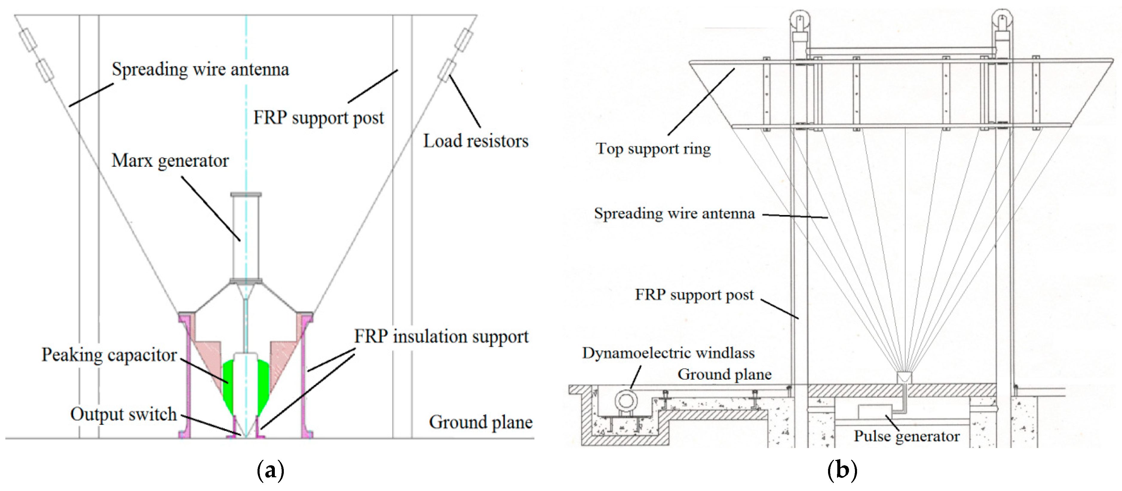
The pulsed power driver used for EMP simulators generally consists of three parts: a primary energy storage unit, a pulse compression unit, and an antenna coupling unit. The Marx generator is a conventional high-voltage pulse-generating device that generates high-voltage electrical pulses through the serial discharge of multiple charged capacitors via multiple gas switches. Due to its many advantages, such as simplicity, reliable performance, easy adjustment, and easy maintenance, it has been widely used as a primary energy storage unit in EMP simulation devices [10,14,15]. Especially with the development of a low inductance fast Marx generator, the pulse driver based on the first-stage steepening mode and the Marx generator has been widely used in the small- and medium-sized EMP simulation devices, with output voltage levels ranging from hundreds of kilovolts to megavolts [11,12,16]. There are two types of driver source position layouts: above the conductive plane and inside the conical antenna (known as top feed, as illustrated in Figure 1a) and below the conductive plane (known as bottom feed, as shown in Figure 1b).
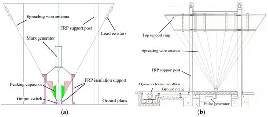
Figure 1.
The structure of a dipole EMP simulator with the ground as the conductive plane. (a) Voltage feed-in over the ground. (b) Voltage feed-in under the ground.
3. Design and Construction
Regardless of the form of the EMP simulator, it mainly consists of two parts: an antenna serving as an electromagnetic energy emission unit and a pulsed power driver serving as an energy supply unit. The working process of the entire device is as follows: the pulsed power driver compresses the slowly charged electric energy into a high-voltage fast pulse in the nanosecond range, which is then fed into the antenna through a connecting port. The antenna converts the electrical pulse into an electromagnetic wave and radiates it outward, forming an EMP environment for experiments.
Taking into account the impact of the surrounding environment on the radiation field, the inverted cone antenna used in the dipole-type EMP simulator is usually built in open areas outdoors and requires a nonconductive support structure to hold it up. Due to environmental factors such as wind, rain, and snow, a wire grid structure, as shown in Figure 1b, is commonly used. When the electromagnetic waves propagate to the top of the inverted cone antenna, reflection occurs. To minimize the impact of reflected waves on the test environment, resistive loading is often applied to the antenna cable to dissipate excess energy.
Based on the above principles, a medium-sized vertical polarized dipole EMP simulator was designed in this paper. The antenna structure is shown in Figure 2, which adopts an inverted cone structure, using the ground as the mirror plane, with a height of 5 m, a half-cone angle of 32°, and an impedance of 75 Ω. The layout of the driving source also adopts two forms, as shown in Figure 1. In the following figure, Figure 2a shows the pulse-voltage top feed mode layout of the simulator, while Figure 2b shows the bottom feed mode layout. In the top feed mode, a one-stage compression circuit consisting of a Marx generator and a peak capacitor is used as the pulse source. For the bottom feed mode, the pulse source is composed of a Marx circuit based on an avalanche tube and a coaxial cable with an impedance of 50 Ω.
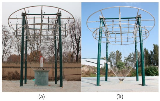
Figure 2.
The developed dipole EMP simulator. (a) Voltage feed-in over the ground. (b) Voltage feed-in under the ground.
3.1. The Vertical Dipole Antenna
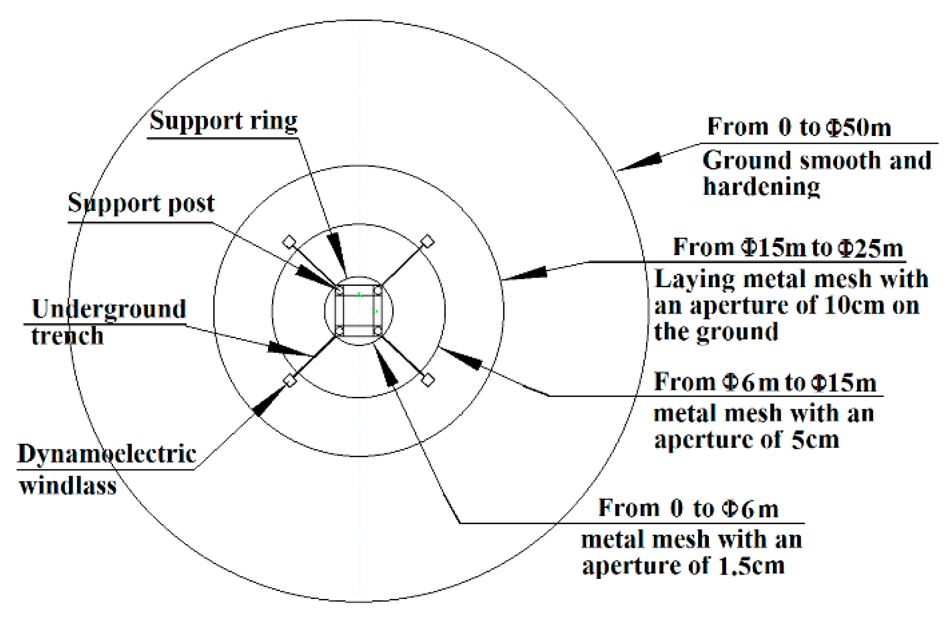
The radiation antenna of our simulator consists of an erection system and a conductive cone, as depicted in Figure 1. The erection system supports and suspends the inverted conical structure of the cone antenna. For this purpose, we use four FRP (Fiber-Reinforced Plastics) columns with a diameter of 200 mm, arranged in a square layout and standing vertically to the ground, as the main body of the erection system. The top crossbeam comprises four FRP pillars with a diameter of 150 mm, overlapped with the four columns perpendicular to the ground to form a stable rectangular doorframe structure. Four dynamoelectric windlasses, evenly distributed around the square support and located on the outer extension line at the diagonal of the ground projection of the four FRP columns, are used to operate the suspension system. Four high-strength insulated cables run along the ground grooves and the inside and outside surfaces of the four columns, connecting the windlasses to a frame cone at the top of the antenna. The conductive cone conducts the pulse current fed in from the driver and generates an electromagnetic field that radiates outward along the conical outer surface. To form the conductive cone of the antenna, we enclose 48 metal wires to create a conical shape instead of using a solid metal cone. The frame cone at the top of the antenna comprises two concentric metal rings and numerous evenly distributed FRP brackets, with a cone angle consistent with that of the antenna, to support the wire-mesh cone and maintain its conical structure. To enhance the electrical conductivity of the ground beneath the antenna and within the effective test area, we need to process the ground accordingly. The design layout of the conductive ground is depicted in Figure 3. Starting from the cone vertex of the inverted cone antenna as the center, we level the surface of the circular area with a diameter of 50 m, followed by a hardening of the cement within the area with a diameter of 25 m, in order to achieve the desired effect.
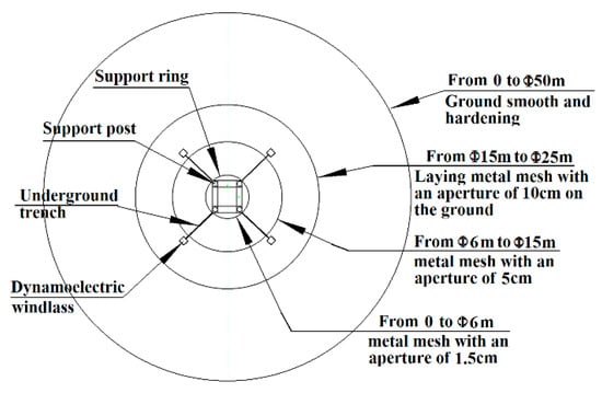
Figure 3.
Top view of ground layout of the developed dipole EMP simulator.
3.2. Pulser Design
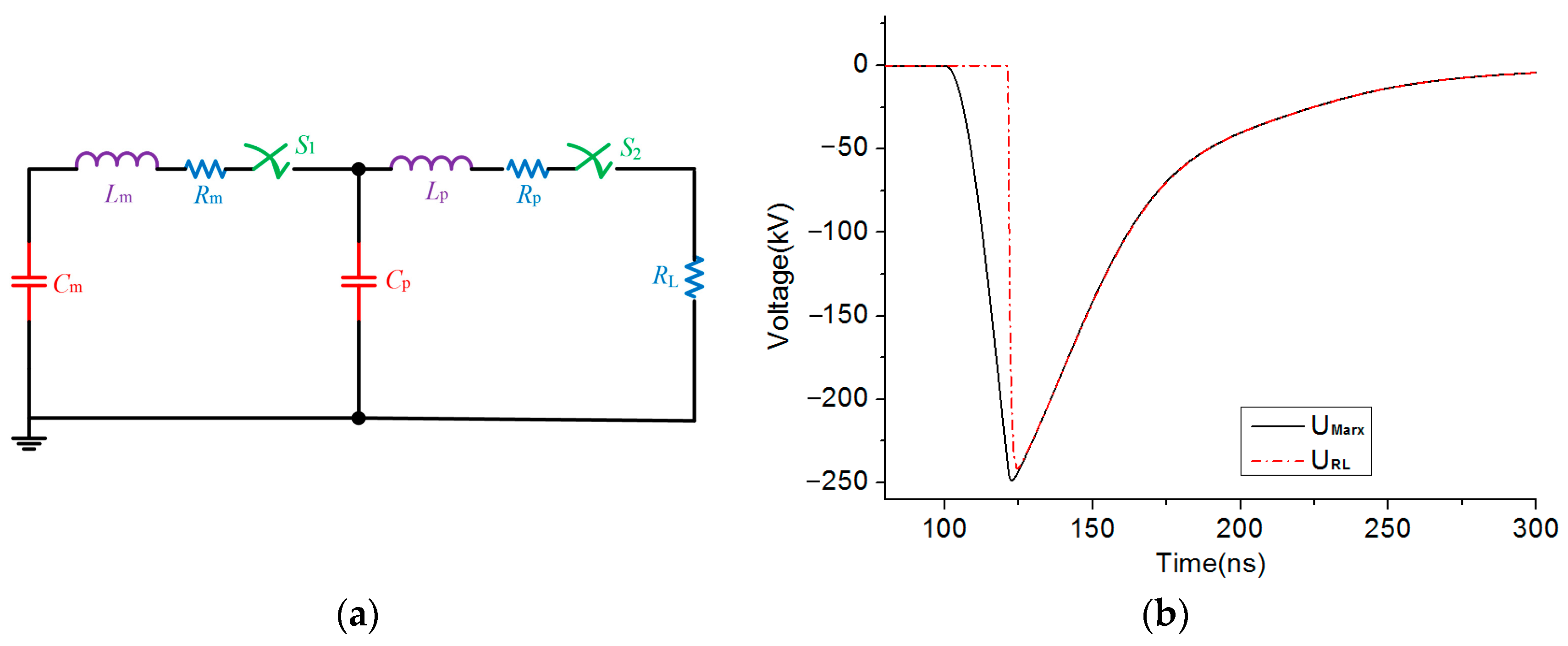
The layout of the pulse voltage top feed mode is presented in Figure 1a and Figure 2a. It features a self-developed compact Marx generator with a rated voltage of 300 kV [12,17] and a peak capacitor [18,19], both arranged on a movable flatbed car. The car is placed in a tunnel, and its upper surface is flush with the ground, being electrically connected to it through several circularly arranged aluminum plates.
The equivalent circuit diagram of this mode is illustrated in Figure 4, where Cm denotes the Marx erection capacitance, Rm and Lm represent the discharging circuit’s equivalent resistance and inductance of the Marx generator, Cp is the peak capacitor, and Rp and Lp are the peak circuit’s resistance and inductance, respectively. RL stands for the load’s equivalent impedance, and S1 and S2 denote the Marx erection and pulse source output switches, respectively, assuming the values of Cm, Lm, Rm, Cp, Lp, Rp, and RL are as follows: Cm = 0.56 nF, Lm = 1.2 μH, Rm = 10 Ω, Cp = 160 pF, Lp = 150 nH, Rp = 10 Ω, and RL = 50 Ω. When S1 is turned on and, approximately 20 ns later, S2 experiences a breakdown, the output voltage waveform of the pulse source is depicted in Figure 4b, and the circuit successfully achieves an ideal double exponential waveform with a rise time of about 2.5 ns and a half-width of approximately 25 ns.
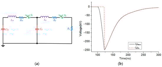
Figure 4.
Equivalent circuit and output waveforms of the pulse source based on one-stage pulse compression. (a) Equivalent circuit of one-stage pulse compression. (b) Simulated output voltage waveforms.
The pulse voltage bottom feed mode is illustrated in Figure 1b and Figure 2b. The pulser used in this mode is a solid-state 6-stage Marx generator based on the avalanche triode [20], consisting of charging isolation resistors, main capacitors, and avalanche triodes. All components are patch components integrated on a PCB board with a size of 130 mm × 44 mm. The output waveform of the pulse source conforms to the double exponential pulse with a rise time of 2.5 ± 0.5 ns and a half-width of 23 ± 5 ns, meeting the specifications of the IEC standard, with a maximum output amplitude of 2.95 kV and an output impedance of 50 Ω. The entire setup is positioned in a tunnel underneath the ground directly beneath the antenna, with the upper end of the tunnel covered with an aluminum plate and connected to the ground. The output voltage pulse is fed into the antenna through the ground plate after being transmitted by a 10-m-long cable with an impedance of 50 Ω.
4. Experiments and Characteristics Research
In an ideal dipole antenna, the electrical pulse input from the pulse source is converted into an electromagnetic wave radiated outward while maintaining all parameters as unchanged. However, in actual engineering implementation, the introduction of supporting structures, wire grid structures, and loading resistors can cause a mismatch of the antenna structure and impedance, resulting in distortion of the waveforms of the electrical pulse input to the antenna and the radiation field generated from the antenna.
To verify whether the simulator’s design meets expectations, it is necessary to measure the parameters of the radiation field and its distribution around the antenna. In order to obtain the best design, it is also necessary to measure the radiation field waveforms at different angles and distances from the antenna origin under different cable numbers of the antenna, different processing methods at the end of the antenna, and different resistive values loaded on the antenna cables. Based on the test results, the impact of the different factors on the simulator’s radiation field waveform and its change rules are analyzed, and it can be used as a basis for the optimization of the simulator’s design.
The experimental setup for measuring the radiation field around the simulator is depicted in Figure 5, where the origin of the coordinate system is taken as the projection of the cone vertex of the inverted-cone antenna, and the z-axis represents the upward direction of the antenna. The x-axis points towards the north and the y-axis towards the west. The vertical polarized electric field component is measured on a radial extension line with different circumference angles. For each measurement, several points at different distances from the antenna’s center in the same direction were chosen, and the field waveform was recorded three times at each point. To ensure the radiation field’s symmetry around the simulator’s circular direction, the number of wire-mesh antenna cables was determined to be 24 to 48 [21]. To meet the measurement requirements, a series of self-developed pulse-electric field measurement systems were used with a bandwidth of 10 kHz to 500 MHz, measuring range of 100 V/m to 1000 V/m, and a background noise of less than 20 mV [22,23,24].
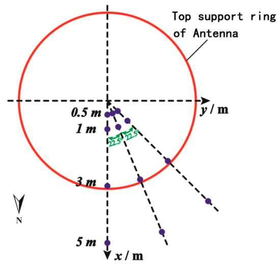
Figure 5.
Test layout of the developed dipole EMP simulator.
4.1. Different Feeding Modes
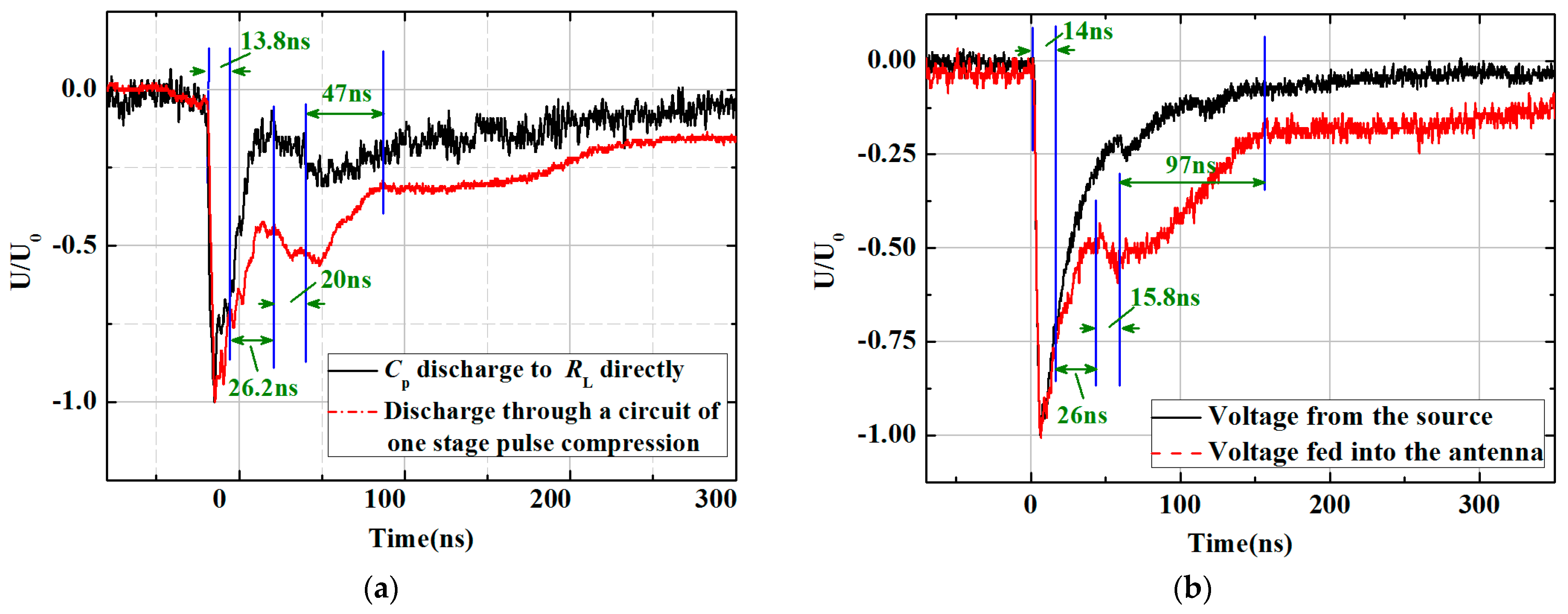
As depicted in Figure 6, the voltage waveforms of the pulse source fed into the antenna under different feed modes were obtained through practical measurements. The waveforms in Figure 6a and the red line in Figure 6b are derived from the measured waveform of the electric field near the antenna origin, while the black curve in Figure 6b represents the output voltage waveform of the bottom feed source when it is directly connected to the 50 Ω matched load. In Figure 6a, the black curve is the output voltage waveform of the peaking capacitor shown in Figure 1a, which is charged by the DC source and discharges directly into the antenna load. On the other hand, the red curve is the voltage pulse generated by a one-stage pulse compression circuit. In this circuit, a voltage pulse is initially formed by the discharge of a compact Marx generator, then compressed by a peaking capacitor, and finally, fed into the antenna load.
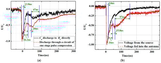
Figure 6.
Voltage waveforms from the source in different feeding modes. (a) Voltage fed into the antenna over the ground. (b) Voltage fed into the antenna under the ground.
The above figures demonstrate that the ideal double exponential wave will experience distortion due to the impedance of the antenna and the structure’s discontinuity. An example of this is shown by the red curve in Figure 6b. The half-width of the pulse begins to widen at a distance of 14 ns from the starting point of the waveform. One possible reason for this is that the antenna cable becomes a resistance-loaded line at a distance of 1 m from the end of the antenna. To achieve this loading method, 12 resistance chains formed by a series of 5 metallized film resistors with equal resistance values replace the original 24 or 48 metal cables and are uniformly distributed along the circumference on the top supporting ring of the antenna, as shown in Figure 1a. The total resistance of the loaded lines equals the impedance of the antenna, and the end of the antenna is left open. In Figure 6, the distance from the field monitoring point to the antenna cone is 0.5 m, the antenna is 5 m high, the wire length from the antenna cone to its end is nearly 6 m, and the electromagnetic wave’s propagation speed in air is approximately 3 × 10⁸ m/s. Based on the principle of electromagnetic wave transmission, it is estimated that it takes around 38 ns for the terminal reflection of the electromagnetic wave at the end of the antenna to reach the measuring point. As seen in Figure 6, this reflection results in a concave in the waveform at the 40 ns position, followed by a bump after 15.8 ns, which is believed to be caused by the reflection of the current wave along the antenna from the cone to the end. Another depression appears on the waveform after 97 ns, which may be caused by the waveform back to the source reflected back and forth again. In Figure 6a, a pit appears 50 ns after the second wave peak, which is just the same as the length of the feed-in cable connected with the pulse source output terminal in the bottom feed mode. Due to the open end of the antenna and the remaining charge on the antenna that cannot be released directly, the time for the waveform to decay to zero at the end of the curve is significantly extended. Overall, it is clear that the discontinuity of the antenna structure and impedance are major factors causing waveform distortion when the ideal double exponential wave is fed into the antenna.
4.2. Influence of the Cable Number of the Wire-Mesh Antenna
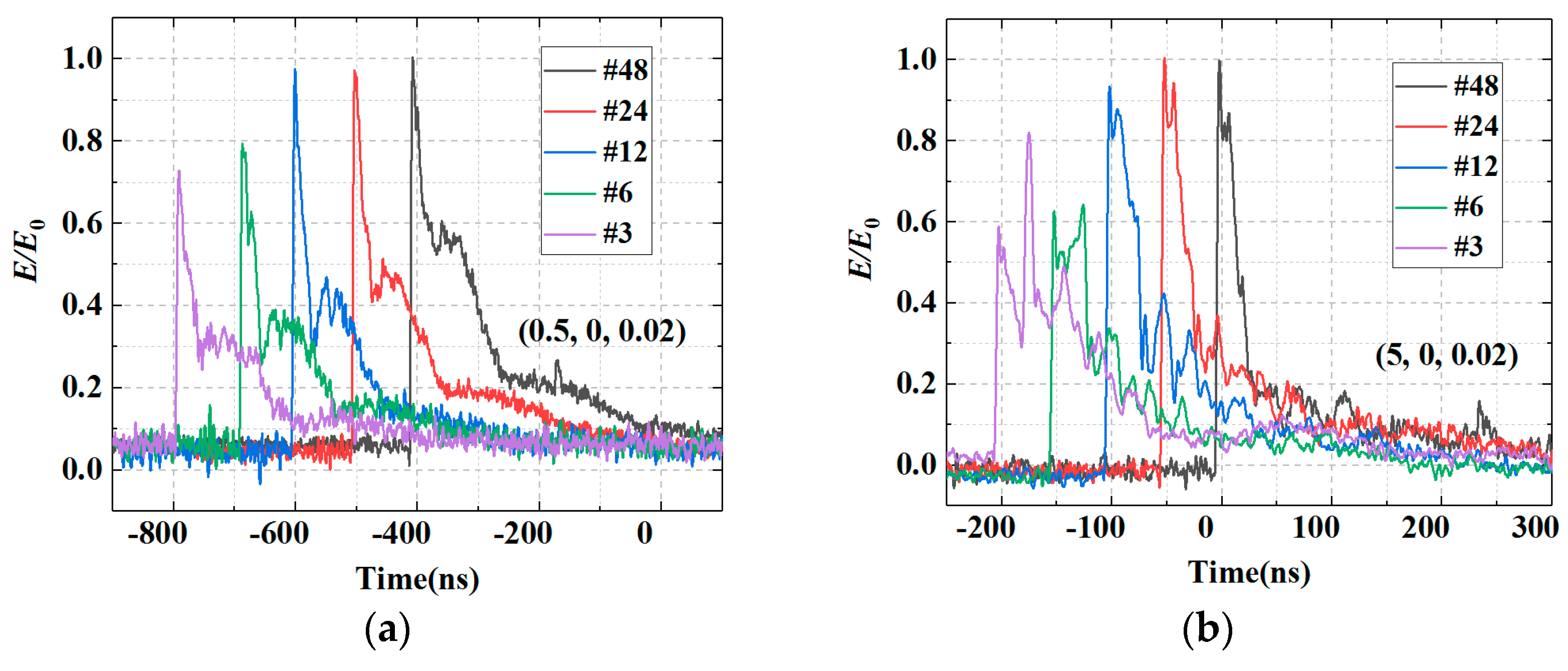
Figure 7 depicts the radiation field waveform variation at different points along the radius extension line in the positive north direction, as well as with different cable numbers of the wire-mesh antenna. It is observed that the amplitude of the radiation field at any given point decreases as the number of antenna cables reduces. Specifically, when the number of cables is less than 12, the decline in the peak value of the radiation field becomes significant. The convergence of wire-mesh antenna cables to the metal cone is shown in Figure 1, with the radiation field waveforms near the cone vertex remaining nearly constant when the number of antenna cables decreases, as illustrated in Figure 7a. However, at points away from the cone vertex, the radiation field waveforms are affected by the change in the number of wire-mesh antenna cables, as shown in Figure 7b. A distortion in the radiation field waveform is evident at the coordinates (5, 0, 0.2) when the number of antenna cables is less than 12. The severity of distortion increases as the number of cables decreases, indicating that the number of antenna lines should not be less than 12. In the subsequent research, the tests were conducted using either 24 or 48 antenna lines.
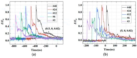
Figure 7.
Influence of the cable number of the wire-mesh antenna on the radiation field of the simulator. (a) Measuring point position: (0.5, 0, 0.02). (b) Measuring point position: (5, 0, 0.02).
4.3. Influence of Antenna End Conditions
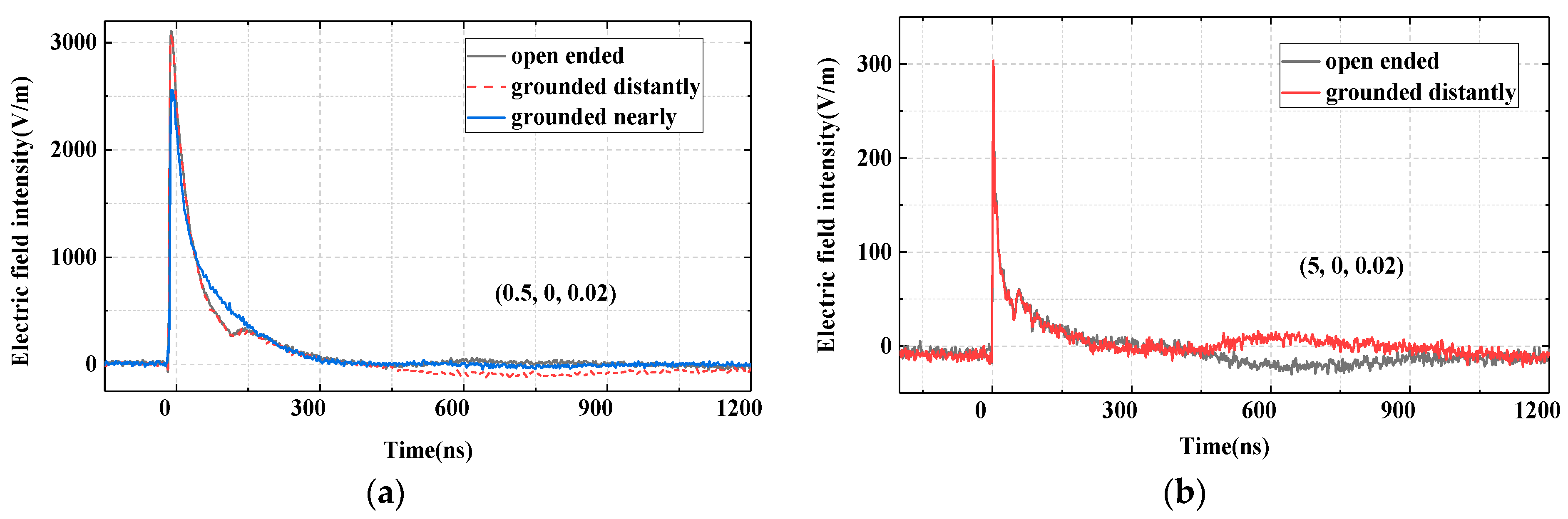
In this paper’s experiment, three different treatment methods were applied to the end of the inverted conical antenna of the simulator: (1) open end, (2) connected to the ground of the laboratory far away from the antenna by a 45-m-long wire, and (3) direct connection of the end of the antenna to the metal mesh below the antenna through a piece of metal wire. The radiation field waveforms measured at different measuring points in the north direction under different antenna terminal conditions are presented in Figure 8. The main waveforms of the radiation field in the open-ended and grounded-distantly cases were consistent, but there were differences at the back ends of the waveforms. Specifically, when the end of the antenna was open, a pit appeared at the end of the waveform at 450 ns. When the antenna was grounded at the far end, a bump appeared at 450 ns at the end of the waveform. This phenomenon is related to the wave reflection caused by the different impedance at the end of the antenna. When the antenna ends were near-grounded, the pit caused by the reflection of the antenna end on the waveforms became less pronounced, and the radiation field waveform became closer to the ideal bi-exponential waveform, as shown in Figure 8a.
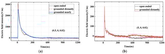
Figure 8.
Influence of the antenna end conditions on the radiation field of the simulator. (a) Measuring point position: (0.5, 0, 0.02). (b) Measuring point position: (5, 0, 0.02).
4.4. Different Angles and Distances
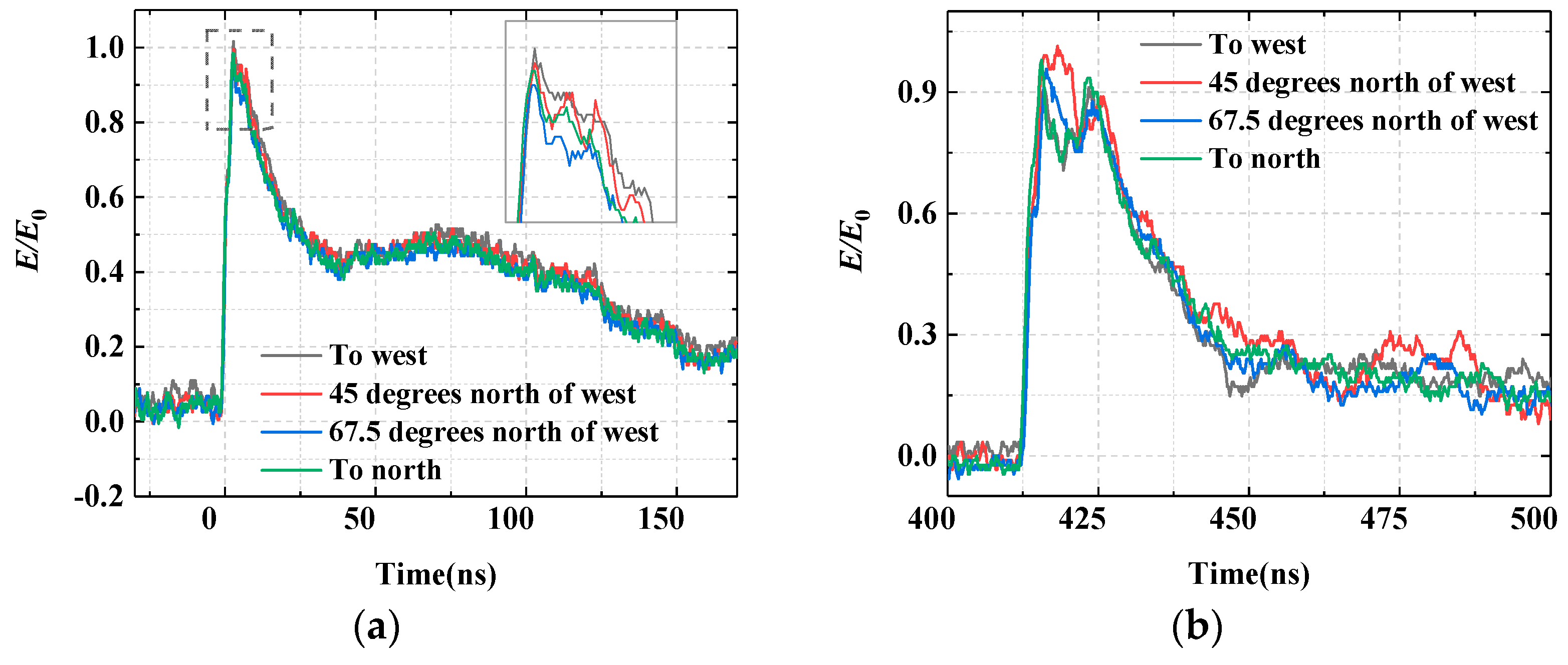
Figure 9 illustrates the radiation field waveforms measured at different angles around the normal of the cone antenna, with the distance between the monitoring point and the antenna cone point kept constant. The waveforms of the radiation field at different distances from the cone vertex are similar when the position of the monitoring point changes with the angle, except for some variations at the peak of the waveform. The connecting line between the cone point and the FRP supporting column of the antenna is oriented at a 45-degree angle north of west. The measuring point of 0.5 m from the antenna cone vertex is located between the connecting line of the cone vertex and the supporting column, whereas the measuring point of 6 m from the cone vertex is located on the extension line of the connecting line between the cone point and the column. As shown in Figure 9a, three distinct peaks appear at the top position of the radiation field waveform measured at the 0.5 m measuring point from the cone point and 45 degrees north of west. The three peaks become less obvious as the measuring point moves closer to the north or west, and the waveform becomes smoother. However, a clear double peak is observed on the waveform of the radiation field when the measuring point is at the position of 6 m from the cone point and the direction of west or north. The pulse width of the first peak of the waveform widens as the measuring point moves closer to the direction 45 degrees north of west, and the amplitude of the second peak decreases. The difference in the radiation field waveform is attributed to the reflection of the wave generated at the antenna’s FRP supporting column. The rise time of the radiation field waveform is only about 2.5 ns, and its shortest wavelength corresponding to the frequency domain is above 80 cm. However, the diameter of the supporting column is only 20 cm. If the FRP column were an ideal insulating medium, its bulk resistivity would be very large, and its dielectric constant would be about 4.5, resulting in a negligible reflection effect. The reason for the observed effect may be that the cement poured into the hollow FRP column to increase its strength also increases the dielectric constant and body conductivity of the supporting column, enhancing its reflection effect on the radiation field.
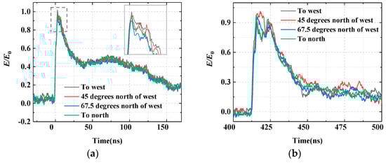
Figure 9.
The radiation field of the simulator on different angles. (a) Distance to the cone point of the antenna is 1 m. (b) Distance to the cone point of the antenna is 6 m.
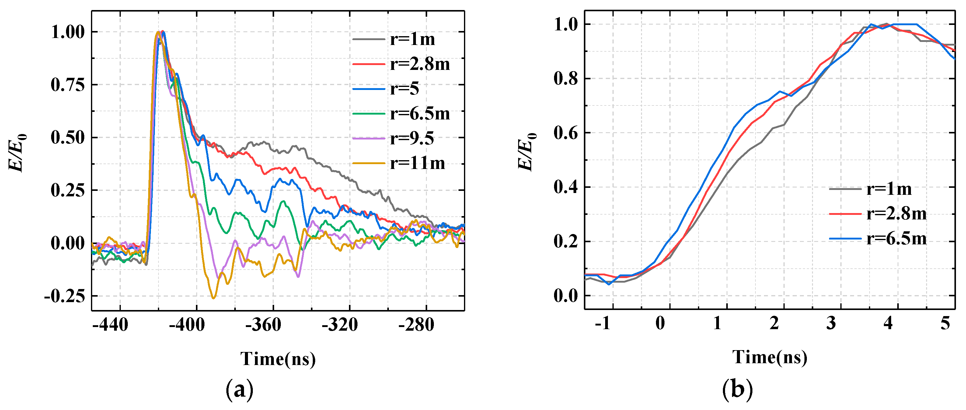
Figure 10 illustrates the radiation field waveforms measured at different distances from the monitoring point to the cone antenna vertex, with a fixed angle around the normal of the cone antenna perpendicular to the ground (at the direction of north). The amplitude of the radiation field measured at the monitoring point, which gradually moves away from the cone point, decreases with the law of 1/r when the distance r varies from 1 m to 11 m. However, the front edge of the radiation field remains basically unchanged, as depicted in Figure 10b. The rise times of the radiation field waveform measured at different positions are all between 2 and 3 ns by adjusting the working state of the internal switches of the pulse source. Specifically, the rise time of the radiation field measured at the position of 2.8 m from the cone antenna vertex is 2.8 ns, and the half-width of the waveform is 24.8 ns. At the 5 m position, the front edge of the measured radiation field is 2.4 ns, and the half-width is 22.8 ns. These measured waveform characteristics conform to the EMP experimental waveform specifications in the IEC61000-2-9 standard [7].
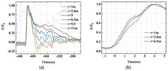
Figure 10.
The radiation field of the simulator on different distances. (a) E waveforms with different distances to the origin of the antenna. (b) The rise time of the E waveforms.
Figure 10a demonstrates that, as the monitoring point moves away from the cone point, the bump appearing on the back edge of the measured waveform of the radiation field gradually disappears. When the distance from the measuring point to the cone point reaches more than 9.5 m, the back edge of the radiation field waveform drops sharply and forms a negative peak. This phenomenon occurs because the current wave reaches the end of the ground net at 12.5 m from the cone vertex when it propagates outward along the metal ground net of the antenna, where the conductivity of the ground will change sharply. As a result, a negative reflection wave is formed. The closer it is to the end of the ground net, the earlier the time of the reflection wave superimposed on the main waveform, and the more obvious the weakening effect on the back edge of the waveform. The advantage of this result is that the shape of the radiation field waveform is closer to the ideal double exponential waveform.
4.5. Resistance Loading on Antenna
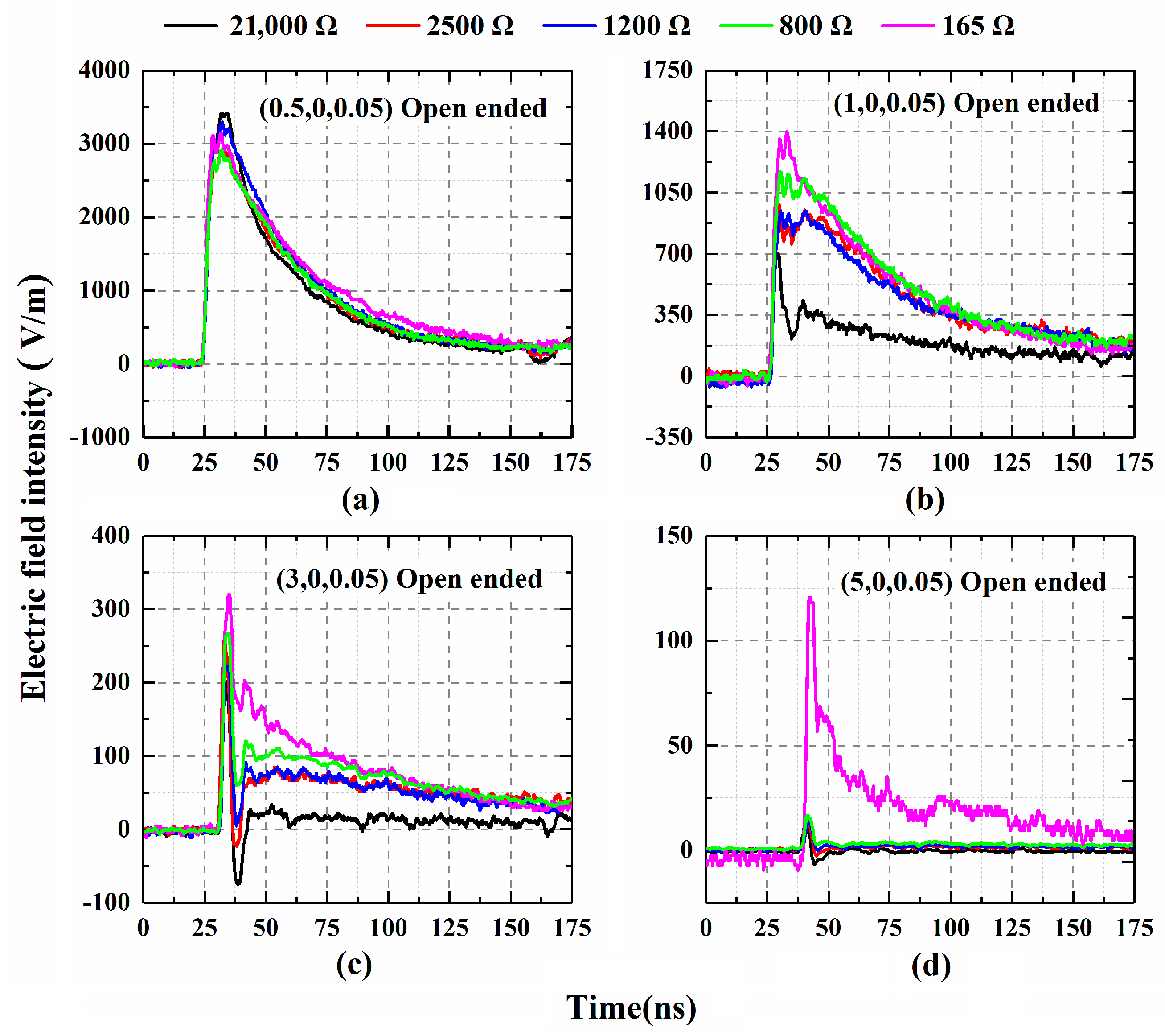
The radiation field waveform produced by small- or medium-sized EMP simulators is inevitably affected by reflection at the end of the antenna due to limitations in the antenna’s structure and size. One way to reduce this reflection effect is to load the resistance onto the antenna’s current-carrying wires [25,26]. To study the effect of resistance loading on the radiation characteristics of the antenna, 48 metal wires of the wire-mesh antenna were replaced with 24 tubular long water resistors with a 15 mm diameter. The resistance value of the water resistor can be adjusted by changing the conductivity of its internal electrolyte. Figure 11 shows the variations of the radiation field waveform measured at different measuring points in the north direction when the water resistance value is changed. The water resistance value indicated in Figure 11 is the total resistance of the 24 water resistors in parallel, which was measured by the bridge.
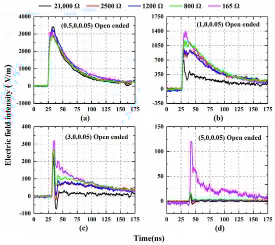
Figure 11.
Effect of antenna resistance loading on a radiation electric field at different measuring points in the north direction. (a) Measure point: (0.5, 0, 0.05). (b) Measure point: (1, 0, 0.05). (c) Measure point: (3, 0, 0.05). (d) Measure point: (5, 0, 0.05).
In Figure 11, it is evident that the radiation field waveform generated by small- or medium-sized EMP simulators is influenced by the reflection at the end of the antenna due to its structure and size limitations. To minimize this reflection effect, a common approach is to load the resistance onto the antenna’s current-carrying wires. In this study, 48 metal wires of the wire-mesh antenna were replaced with 24 tubular long water resistors to investigate the impact of resistance loading on the antenna’s radiation characteristics. The resistance value of the water resistor was adjusted by modifying the conductivity of its internal electrolyte.
The results indicate that, at a distance of 0.5 m from the antenna cone vertex (as shown in Figure 11a), the radiation field waveform closely resembles the ideal double exponential wave without any concave or protruding features caused by antenna end reflection (as shown in Figure 6). When the resistance value increases gradually from 165 Ω to 2.1 kΩ, the radiation field waveform remains unchanged, but the amplitude slightly decreases. However, the amplitude of the radiation field decreases gradually with the increasing resistance loaded onto the antenna at the measuring point of 1 m from the antenna cone vertex. When the resistance value reaches 2.1 kΩ, a significant distortion appears on the radiation field waveform, and an oscillation occurs at its peak (as shown in Figure 11b). As the measuring point moves outward to 3 m from the antenna cone vertex, the radiation field waveform starts to distort when the resistance value is greater than 460 Ω, and the pulse width of the waveform is reduced to only a few ns (as shown in Figure 11c). At the 5 m position, none of the resistance values used in the test meet the application’s requirements for the waveform width of the radiation field. Nevertheless, the amplitude of the radiation electric field is still decreasing with the increasing load resistance, because the attenuation effect of the resistance on the current passing through the antenna is enhanced with the increase of the resistance value. This leads to different distortions in the radiation field waveform measured at different points.
It is worth noting that the parameters of the radiation field waveform at the measuring point (0.5,0,0.05) below the solid metal cone of the antenna are mainly determined by the transmission characteristics of the single-cone antenna. Hence, the impact of the water resistance loaded above the metal cone of the antenna is insignificant. Therefore, the radiation field waveform measured at this point is essentially consistent across different resistance values. As the current propagates outward along the resistance line loaded onto the antenna, the radiation efficiency of the simulator decreases gradually with the increasing resistance value due to continuous energy dissipation. Consequently, the intensity and pulse width of the radiation field show a tendency to decrease gradually, and the waveform is distorted accordingly.
4.6. Conclusions
The following conclusions can be drawn from the above experiments and analysis:
- (1)
- The radiation field waveform generated by the developed simulator has a front edge between 2 and 3 ns, a half-width of about 25 ns, and meets the requirements of the EMP test standard. It can be used to carry out EMP-related experimental research. Due to the discontinuity of the actual antenna structure, there will be some distortion in the radiation field waveform compared to the ideal double exponential high-voltage pulse signal fed from the driving source. However, it will not have a significant impact on the important indicators of the radiation field waveform, such as the front edge and the half-width.
- (2)
- The amplitude of the electromagnetic radiation field at the same measuring point around the wire grid antenna will gradually decrease as the number of antenna cables decreases. When the number of cables is reduced to less than 12, the radiation field waveform will undergo severe distortion and no longer meet the requirements of the test standard. When the number of the antenna cables is set to 24 or above, the radiation field waveform remains basically unchanged.
- (3)
- The electromagnetic radiation field generated by the ideal inverted cone antenna will have an isotropic distribution along the circumference, with the vertex of the cone as the center. Along the radial direction, the amplitude of the radiation field will decay according to the 1/r rule as the monitor moves away from the conical point of the antenna, while the waveforms of the radiation field remain unchanged. However, in the actual engineering implementation process, due to the presence of the support system, there may be some differences in the radiation field waveform at different angles on the same circumference and at different distances near the support column, but this does not affect the main parameters of the radiation field, such as the front edge and half-width.
- (4)
- When the current wave fed into the antenna reaches the top of the inverted cone antenna and the outer edge of the conductive plane on the ground, it will cause a distortion of the radiation field waveform due to the sudden change in the conductive impedance. When the measuring point is far away from these two locations, this distortion mainly manifests itself in the trailing edge of the radiation field waveform, with little effect on its leading edge and half-width. Therefore, when the antenna end is treated with three different methods of grounded-nearly, grounded-distantly, and open-ended, the radiation field waveform in the test area is basically unaffected, only slightly different at its trailing edge. The loading resistance on the antenna cable can reduce the impact of the reflection caused by the structural discontinuities on the radiation field waveform. However, selecting a resistance value that is too large may cause a decrease in the amplitude of the radiation field or even severe waveform distortion. Therefore, when using this method, sufficient argumentation is required.
5. Summary
This paper presents a medium-sized vertical dipole radiating EMP simulator, including its design and experimental results. The antenna has an inverted cone structure with a half-cone angle of 32° and a height of 5 m. The simulator has two pulse feeding modes, which can switch quickly and conveniently for different experimental purposes. The experimental region is a circular ground 25 m in diameter around the cone vertex of the antenna. The variations of the radiation field generated by the simulator under different feed modes, different numbers of the wire-mesh antenna lines, different terminal conditions of the antenna, different measurement angles and distances, and the resistance loading on the antenna are studied experimentally. The experimental results show that the rise time of the radiation field waveform generated by the simulator can be up to 2–3 ns, and its half-width is about 25 ns, meeting the requirements of the EMP experiment waveform for the IEC61000-2-9 standard. This simulator can be used for radiation characteristic research, field measurement system calibrations, EMP effect research, and more.
Author Contributions
Investigation, W.J., K.M., L.C., Z.C., F.G., Y.W., L.S., W.W. (Wei Wang), Y.S., X.Z., G.W. and Y.L.; Data curation, W.J., K.M. and L.C.; Writing—original draft, W.J.; Writing—review & editing, W.J.; Supervision, W.W. (Wei Wu). All authors have read and agreed to the published version of the manuscript.
Funding
This research received no external funding.
Data Availability Statement
Data is unavailable due to privacy or ethical restrictions.
Conflicts of Interest
The authors declare no conflict of interest.
References
- Qiu, A. Application of Pulse Power Technology; Shaanxi Science and Technology Press: Xi’an, China, 2016. [Google Scholar]
- Zhou, B.; Chen, B.; Shi, L. EMP and EMP Protection; National Defense Industry Press: Beijing, China, 2003. [Google Scholar]
- Jia, W.; Chen, Z.; Guo, F.; Xie, L.; Yang, T.; Tang, J.; Jin, T.; Qiu, A. Drivers of small and medium scale electromagnetic pulse simulator based on Marx generator. High Power Laser Part. Beams 2018, 30, 073203. [Google Scholar] [CrossRef]
- Giri, D.V.; Prather, W.D. High-altitude electromagnetic pulse (HEMP) risetime evolution of technology and standards exclusively for E1 environment. IEEE Trans Electromagn. Compat. 2013, 55, 484–491. [Google Scholar] [CrossRef]
- Qiao, D.J. Introduction to HPEMP, IEME, EMC, and EM Susceptibility and Its Assessments. Mod. Appl. Phys. 2013, 9, 219–224. [Google Scholar]
- Gao, H.L.; Zhang, Z.Q.; Gao, D.P.; Zhang, Z.; Yin, S.; Ding, Y. Generation of high-power electromagnetic pulses and its application to radiation effect research: A review. Sci. Sin. Phys. Mech. Astron. 2021, 51, 092007. (In Chinese) [Google Scholar] [CrossRef]
- IEC 61000-2-9; Electromagnetic Compatibility (EMC)—Part 2–9: Description of HEMP Environment—Radiated Disturbance—Basic EMC Publication. International Electrotechnical Commission: Geneva, Switzerland, 1996.
- IEC 61000-4-32; Electromagnetic Compatibility (EMC)—Part 4–32: Testing and Measurement Techniques—High-Altitude Electromagnetic Pulse (HEMP) Simulator Compendium. International Electrotechnical Commission: Geneva, Switzerland, 2002.
- Giles, J.C.; Prather, W.D. Worldwide High-Altitude Nuclear Electromagnetic Pulse Simulators. IEEE Trans Electromagn. Compat. 2013, 55, 475–483. [Google Scholar] [CrossRef]
- Bailet, V.; Carboni, V.; Eichenberger, C.; Naff, T.; Smith, I.; Warren, T.; Whitney, B.; Giri, D.; Belt, D.; Brown, D.; et al. A 6-MV Pulser to Drive Horizontally Polarized EMP Simulators. IEEE Trans Plasma Sci. 2010, 38, 2554–2558. [Google Scholar] [CrossRef]
- Jung, M.; Weise, T.; Nitsch, D.; Braunsberger, U. Upgrade of a 350kV NEMP HPD Pulser to 1.2MV. In Proceedings of the 26th International Power Modulator Symposium, San Francisco, CA, USA, 23–26 May 2004. [Google Scholar] [CrossRef]
- Jia, W.; Li, J.; Guo, F.; Xie, L.; Tang, J.; Zhang, G.; Chen, W.; Xie, Y. A 500KV Pulser with Fast Risetime for EMP Simulation. In Proceedings of the IPAC2013, Shanghai, China, 12–17 May 2013; pp. 708–710. [Google Scholar]
- IEC61000-4-25; Testing and Measurement Techniques—HEMP Immunity Test Methods for Equipment and Systems. International Electrotechnical Commission: Geneva, Switzerland, 2001.
- Smith, I.D. The pulse power technology of high altitude EMP simulators. In Proceedings of the Symposium and Technical Exhibition on Electromagnetic Compatibility, Zurich, Switzerland, 8–10 March 1983. [Google Scholar]
- Gilman, C.; Lam, S.K.; Naff, J.T.; Klatt, M.; Nielsen, K. Design and performance of the FEMP-2000: A fast risetime, 2 MV EMP pulser. In Proceedings of the 12th IEEE International Pulsed Power Conference, Monterey, CA, USA, 27–30 June 1999; pp. 27–30. [Google Scholar] [CrossRef]
- Schilling, H.; Schluter, J.; Peters, M.; Nielsen, K.; Naff, J.T.; Hammon, H. High voltage generator with fast risetime for EMP simulation. In Proceedings of the 10th IEEE International Pulsed Power Conference, 3–6 July 1995; pp. 1359–1364. [Google Scholar] [CrossRef]
- Xie, L.; Jia, W.; Guo, F.; Chen, W.; Zhang, G.; Jin, T. Development of an 100 kV compact Marx generator. High Power Laser Part. Beams 2016, 28, 045016. [Google Scholar] [CrossRef]
- Chen, Z.-Q.; Ji, S.-C.; Jia, W.; Zhu, X.-Q.; Liang, T.-X.; Guo, F.; He, X.-P.; Wei, W. A coaxial film capacitor with a novel structure to enhance its flashover performance. Rev. Sci. Instrum. 2019, 90, 124709. [Google Scholar] [CrossRef] [PubMed]
- Zhiqiang, C.; Wei, J.; Junping, T. An Optimal Design Method for Structural Parameters of Coaxial Film Capacitors. Modern Appl. Phys. 2019, 10, 41–47. [Google Scholar]
- Cheng, L.; Chen, Z.; Wang, H.; Guo, F.; Xie, L.; Xiao, J.; Wang, Y.; Shen, S.; Ding, W. A novel avalanche transistor-based nanosecond pulse generator with a wide working range and high reliability. IEEE Trans. Instrum. Meas. 2021, 70, 9002714. [Google Scholar] [CrossRef]
- Zhu, X.; Wu, W.; Jia, W. Radiation characteristics of wire vertically polarized EMP radiating-wave simulator fed by coaxial transmission line with 4 m height. Modern Appl. Phys. 2021, 12, 020503. [Google Scholar]
- Shi, Y.; Wang, W.; Zhu, Z.; Yang, J.; Nie, X.; Cheng, Y. A Bias Controllable Birefringence Modulation Measurement System for Sub-nanosecond Pulsed Electric Field. IEEE Trans. Instrum. Meas. 2021, 70, 6004311. [Google Scholar] [CrossRef]
- Shi, Y.; Nie, X.; Zhu, Z.; Wang, W.; Yang, J.; Sun, B.; Wang, J. Study of the Fitting Method in the Sensitivity Calibration of a HEMP Measuring System. IEEE Trans. Electromagn. Compat. 2020, 62, 1179–1185. [Google Scholar] [CrossRef]
- IEEE STD1309-2005; IEEE Standard for Calibration of Electromagnetic Field Sensors and Probes Excluding Antennas from 9 kHz to 40 GHz. IEEE: New York, NY, USA, 2013.
- Maloney, J.G.; Smith, G.S. Study of transient radiation from the Wu-King resistive monopole-FDTD analysis and experimental measurements. IEEE Trans. Antennas Propag. 1993, 41, 668–676. [Google Scholar] [CrossRef]
- Wraight, A.; Prather, W.D.; Sabath, F. Developments in Early-Time (E1) High-Altitude Electromagnetic Pulse (HEMP) Test Methods. IEEE Trans. Electromagn. Compat. 2013, 55, 492–499. [Google Scholar] [CrossRef]


Disclaimer/Publisher’s Note: The statements, opinions and data contained in all publications are solely those of the individual author(s) and contributor(s) and not of MDPI and/or the editor(s). MDPI and/or the editor(s) disclaim responsibility for any injury to people or property resulting from any ideas, methods, instructions or products referred to in the content. |
© 2023 by the authors. Licensee MDPI, Basel, Switzerland. This article is an open access article distributed under the terms and conditions of the Creative Commons Attribution (CC BY) license (https://creativecommons.org/licenses/by/4.0/).