Analysis of Core Losses in Transformer Working at Static Var Compensator

Abstract

This article presents the comparison of 3D and 2D finite element models of a power transformer designed for reactive power compensation stations. There is a lack of studies in the literature on internal electromagnetic phenomena in the active part of a transformer operated in these conditions. The results of numerical 2D and 3D calculations of no-load current and losses in the transformer core were obtained by using various methods and models. The impact of considering the hysteresis loop phenomenon on the calculation of core losses was investigated by using the Jiles–Atherton core losses model. The results obtained in the paper show that the model of the core must contain the areas representing the influence of overlappings on the no-load current and also on the flux density field in the core. The capacitive load of the transformer increases the flux density in the core limbs by several percent, so the power losses there must also increase accordingly. As a summary of the research, differences in the values of losses in each core element between the capacitive load and no-load conditions are presented. The results presented in this paper indicate that considering nonlinearity related to the magnetic hysteresis loop has a significant impact on the calculation of the core losses of power transformers.

1. Introduction

The development of the world power supply makes it necessary to search for better methods to regulate the current flow and voltage level. Static var compensation (SVC), which belongs to the group of flexible alternating current transmission systems (FACTS), has gained great importance.

The technical solutions of SVC, which can be found in the literature [1], allow one to present the basic elements of this system, which are a load for the power transformer. The thyristor-switched capacitor (TSC) is a system in which each section contains, in addition to capacitors, thyristor switches that are turned on or off depending on the required reactive power. Thyristor-switched reactors (TSR) or thyristor-controlled reactors (TCR) consist of several three-phase sections in which thyristor switches control the inductive elements by turning them on or off depending on the reactive power that the entire compensation system must draw from the power grid. Fixed capacitors (FC) are also used in SVC stations as filters for higher harmonics. The presence of FC is necessary to eliminate interference caused by semiconductor switches.

The element that connects the reactive power compensation system to the high-voltage network (HV) is a power transformer. Its design must ensure the ability to transform reactive power. In addition, due to the operation of semiconductor switches, the power transformer must be able to handle harmonic currents and maintain voltage levels associated with all operating conditions without loss of life [2]. The basic structure scheme of the SVC reactive power compensation station is presented in Figure 1.

One of the most important aspects to consider, when analyzing the operation of a power transformer in a SVC station is the capacitive load. In the presence of a capacitive load, the voltage on the secondary side and the magnetic flux density may increase [3]. The explanation of this phenomenon is presented in Figure 2.

An important point in the design of the core, in connection with the determination of its cooling parameters, is the analysis of the worst-case operating conditions of a power transformer, i.e., overexcitation and loads that lead to an increase in the core hot-spot temperature. These conditions are specified in the applicable industry standards. In a power transformer with three wounded limbs, the core hot spot is located in the geometric center of the overlap area between the top yoke and the center limb [4].

The inrush current is a form of overload that occurs when the power transformer is energized. The phenomenon occurs mainly when the voltage exceeds the value zero and when the transformer has not been switched off after its previous operation by a smooth reduction to a voltage of 0 V, leaving residual magnetic flux in the core. The inrush current is transient, and the time constant of the transient state after connecting the power transformer to the HV network depends on the characteristics of the magnetic circuit. It can last up to 1 s. Details of the power transformer inrush current calculations can be found in [5].

2. Analysis of Magnetic Field and Core Losses

The analysis of magnetic field distribution and the core losses is an essential part of the power transformer design process. Therefore, the selection of an appropriate calculation method that takes into account the hysteresis phenomenon is necessary for their correct determinations [6]. The most popular models for the calculation of core losses are comprehensively presented in [7,8]. A large group of empirical models is based on the equation that was proposed in 1982 by C. Steinmetz in [9]. In this method, the time-averaged core losses per volume P are expressed as an exponential function of peak magnetic flux density and frequency, which has the following form:

$$P=k·f^{\alpha }·B_m{}^{\beta }$$

(1)

The symbol k denotes a material parameter, f is the frequency, B_m is the peak magnetic flux density, and α and β are empirical coefficients, which are determined by fitting the model to the loss measurement data.

One of the most common models for calculating power losses in transformer cores is the Jiles–Atherton (J-A) hysteresis loop model presented in [10]. It is a mathematical nonlinear model that represents the relationship between the magnetic field strength and the magnetization at a given time. The J-A model is based on the theory that the magnetization M in ferromagnets depends not only on the strength of the magnetic field but also on the magnetization history of the material. In the J-A model, five coefficients are used to characterize the ferromagnetic material [11]. In practice, the generation of the hysteresis loop consists in the selection of the coefficients based on the power loss of the modeled core sheet for the frequencies of 50 Hz and 60 Hz and its magnetization curve. An example of the result of generating the hysteresis loop of the J-A model is shown in Figure 3.

In the scientific literature [12,13,14,15], there are many examples of the application of a numerical analysis of power transformers using commercial packages that employ the finite element method (FEM). In this paper, Simcenter MAGNET 2022.1 was selected to simulate phenomena in the power transformer. This software uses the FEM to solve the 2D form of equation 2 for the magnetic potential.

$$rot \left(\frac{1}{\mu } rot A\right)=J$$

(2)

where μ—magnetic permeability, A—magnetic potential vector, and J—current density vector.

In this method, the problem domain is divided into a mesh of triangular elements, and the potential in each element is approximated by a simple function of x and y coordinates. Eddy currents are not considered in these calculations. The 3D formulation is based on the T-Ω method presented in [16]. The magnetic field is represented as the sum of two parts: the gradient of a scalar potential magnetic field Ω and, in conductors, an additional vector field T represented with vector-edge elements. In this method, Equation (3) incorporating Faraday’s law and Equation (4), which takes into account source lessness of the H field, are solved.

$$rot \left(\frac{1}{\gamma } rot T\right)=-\frac{d}{dt} \left[\mu \left(T-grad \mathsf{\Omega }\right)\right]$$

(3)

where γ—conductivity.

$$div \mu \left(T-grad \mathsf{\Omega }\right)=0$$

(4)

Two available software solvers were used for the power transformer simulations: Time-Harmonic, in which the analysis is performed at a given frequency and non-linear properties of the ferromagnetic elements are approximated, and Transient, which is based on the time-stepping method, in which Maxwell’s equations are solved. The electromagnetic field is decomposed into discrete time steps, and Maxwell’s equations are solved iteratively at each step [17]. In this way, it is possible to analyze phenomena at specific time points. Both the Steinmetz and J-A models are used to calculate the core losses, although the J-A model can only be used with the Transient solver and 2D models.

3. Numerical Model of Transformer Core and Winding

Electromagnetic calculations were performed for a 300 MVA power transformer, whose main electrical parameters are HV 230 kV (wye connection) and LV 45.5 kV (delta connection). After analyzing the dimensions of the transformer, a three-dimensional finite element model was created. Considering the fact that the objective of the analysis was to determine the distribution of magnetic flux and calculate the core losses, the finite element mesh must be dense enough to achieve satisfactory accuracy. The 3D mesh of the power transformer is shown in Figure 4b. Figure 5 presents a circuit diagram of the analyzed transformer under a capacitive condition.

4. Results of 3D and 2D Analysis of Power Transformer

The analysis of the no-load state of the 3D model of the power transformer was performed using the Time-Harmonic solver. In the three-dimensional model, the region of the core sheet overlap was not considered due to the high degree of complexity of this issue. Performing a 3D analysis using the time-stepping method in the case of a 3D core model required an enormous amount of computing time.

Figure 6 presents the calculation results showing the distribution of flux density in the core of the power transformer at no-load. Attention is drawn to the region where the root mean square value (RMS) of magnetic flux densities exceeds 6T. It was found that such values occur only near the vertices of the individual mesh elements in the corners of the core window. This is a numerical calculation error that has a minimum impact on the overall parameters, such as no-load current or power losses in the core.

The analysis of the limb cross-section shows that the magnetic flux in the transformer core is distributed evenly. The RMS value of the magnetic flux densities in the middle point of the limb is B_RMS = 1.15 T which gives the maximum value B_max = 1.63 T.

In the case of a 2D analysis of the load condition of a power transformer, it is necessary to scale the model, calculate the corresponding depth of the geometry and determine the scaling factor of the magnetic permeability. The criterion for similarity between the 2D model and the 3D model is the magnitude of the stored energy of the magnetic field in the whole object. This is possible if the magnetic field strength is identical in both the 2D and 3D models. Under load conditions of the power transformer, most of the magnetic field energy is concentrated in the winding zone, which is in the duct between the HV and LV windings. Therefore, it is required in the 2D model to resolve the value of the magnetic permeability of the winding zone area by the scaling factor expressed in Equation (5):

$$\frac{{\mu }_{2Dk}}{{\mu }_{3Dk}}=\frac{d_k}{d}$$

(5)

where μ_2Dk—magnetic permeability of the k area of the 2D model, μ_3Dk—magnetic permeability of the k area of the 3D model, d_k—limb cross-section divided by its diameter, and d—depth of the 2D model. A detailed explanation of this issue can be found in [18,19].

In order to determine the scaling factor for the magnetic permeability in the area of the winding zone, the depth of the 2D model was chosen to correspond to the real cross-section of the core. The rescaling of the magnetic permeability increases the value of the leakage flux, resulting in a good agreement between the magnetic fluxes entering the core calculated by two and three-dimensional models. The value of the magnetic permeability in the overlapping area was calculated as accurately as possible using measurements of the real no-load current. Figure 7 presents an example of the core sheet overlapping area. The 2D model of the power transformer and the finite element mesh are shown in Figure 8.

In addition to the periodic component, the inrush current also contains an aperiodic component whose value depends on the phase of the voltage at the time the transformer is turned on. The sum of the instantaneous aperiodic components of the three phases causes the magnetization of the transformer core with a random vector in space. To minimize this phenomenon, it was assumed that the supply voltage increases exponentially to the nominal value during transformer turn on. Function (6) was used for this purpose.

$$u\left(t\right)=\left(1-e^{-\frac{t}{\tau }}\right) · U_m · e^{j\omega t}$$

(6)

where t—time instant (ms), τ—time constant, assumed τ = 20 ms, ω—pulsation, and U_m—maximum voltage value (V).

Due to the relatively rapid increase in voltage values in successive periods, there is an aperiodic component present in the calculations. A comparison was made between the values of the phase currents in the no-load state obtained in the test field and the values calculated in the software using the time-stepping method with time steps equal to 0.1 ms. The current waveform in the 2D model of the power transformer for the time-stepping method, using the Steinmetz and J-A core losses models, is presented in Figure 9.

To check the accuracy of the numerical model of the 300 MVA transformer, the no-load inrush current obtained from the test field was compared with the RMS values of the current waveform calculated using Time-Harmonic 2D and Transient 2D models with Steinmetz and Jiles–Atherton core losses models. The results are displayed in Figure 10.

The best convergence with the measured no-load currents in the test field was obtained for the Transient 2D method, using the J-A core losses model with a range of 5 to 21% for individual phases. The results of the RMS values of the transformer no-load currents differ between the windings on the outer limbs. The main factors affecting this are differences in the properties of the core laminations and unavoidable production tolerances that determine the allowable differences in the dimensions of air gaps in the overlap region. The waveform of the current in LV windings under capacitive load conditions was also analyzed. The current harmonic inserted by the additional current sources on the secondary side had no effect on the flux density inside the core.

The differences between the values of the no-load losses of the real transformer measured in the test field and the calculated values in the software are presented in Figure 11. The difference expressed as a percentage is placed on the ordinate axis, while the successive calculation methods with core losses models are placed on the axis of abscissa.

Based on the differences, the Transient 2D method using the J-A core losses model and the Time-Harmonic 3D method with the Steinmetz model show the best convergence with the measurements of the real unit. However, the good accuracy of the 3D Time-Harmonic results seems to be accidental because the model does not contain overlapping.

To compare the differences between the core losses in the no-load state and in the capacitive load state, Figure 12 and Figure 13 are displayed, showing the flux density distribution in the 2D model core. The core hot spot was divided into two parts: the part located in the upper yoke (point A) and the part located in the middle limb (point B). In addition, the central part of the middle limb (point C) was also verified. For these points, the maximum flux density at a given moment in time was calculated. Determination of the magnetic flux density distribution was performed using the time-stepping method.

The value of flux density at point C increases significantly in the case of the capacitive loading of the transformer compared to the no-load condition. The flux density also increases in the limb part of the core hot spot (point B), while in the yoke part (point A), the flux density values remain similar. The explanation of this phenomenon is that the leakage flux that occurs under load enters the limbs of the transformer core, resulting in an increase in the magnitude of magnetic flux density in this area. In the yoke section, on the other hand, the additional leakage flux does not occur. For both investigated operating states of the power transformer, the magnitude of flux density in the core hot spot is significantly higher compared to the other parts of the core.

The analysis of the differences in core losses between the capacitive load and no-load conditions was also performed, examining individual elements of the transformer core. The 2D model of the core was divided into smaller elements numbered from 1 to 11. The results obtained from the Transient 2D method using the J-A core losses model were selected for comparison. The obtained differences were related to the values of core losses in the no-load state. The results, showing the changes expressed as a percentage are presented in Figure 14, maintaining the division into hysteresis and eddy current losses.

The core losses of the transformer in the capacitive load condition increased compared to those calculated for the no-load condition. The largest change in the value of hysteresis losses, amounting to 21%, was observed in element 3, the middle part of the center limb. The percentage change values of more than 10% were also observed in the outermost limbs and in elements 4 and 5, which represent the core hot-spot area in the middle limb.

5. Conclusions

• The obtained results of core losses calculated using various methods showed an accuracy within a few percent of the results obtained from measurements of the real power transformer in the test field. The Transient 2D calculation method with the J-A core losses model and the Time-Harmonic 3D method with the Steinmetz model proved to be the best. It is supposed that in the case of the second method, such a good result is accidental because the 3D model did not consider the region of overlap; moreover, the hysteresis loop was also not included in the calculations. The important issue is that core loss values calculated using the Steinmetz model are subject to an error resulting from the need to extrapolate the magnetic permeability and iron losses characteristic in the saturation area.
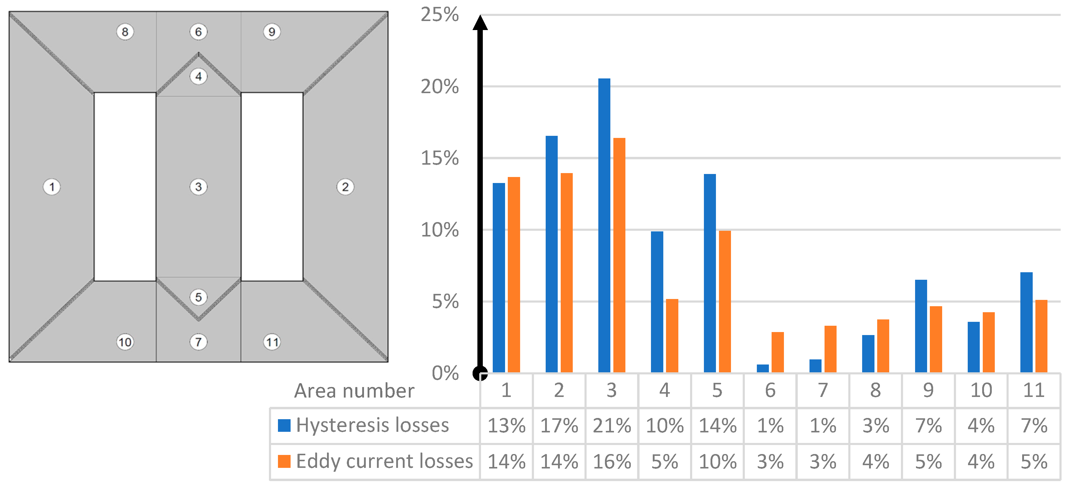
• The presented two-dimensional model of the power transformer was prepared considering the areas where the core sheets overlap. Thanks to this approach, it was possible to obtain a more realistic distribution of flux density in the core as well as the values of phase currents.
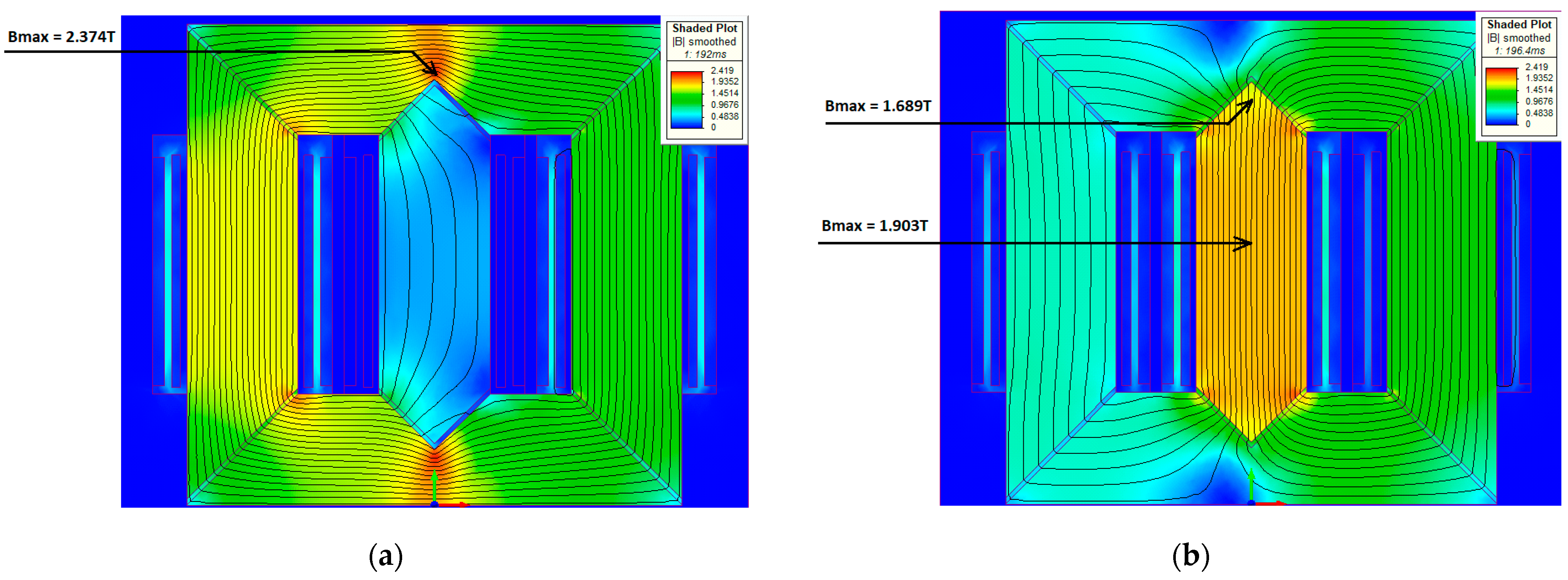
• The analysis of the core hot-spot area and the central point of the core limb showed that the capacitive load causes a significant increase in the value of magnetic flux density in the core limb compared to the value obtained in the no-load condition. The change in flux density was particularly noticeable in the limb part of the core. Considering the preparation of the power transformer design for operation in reactive power compensation stations, an increase in the magnetic flux density value results in the core entering the saturation state more quickly. In areas with the worst oil circulation, local overheating may occur, leading to a weakening of the insulation system. The consequence of this may be a significantly accelerated aging of the power transformer, resulting in increased operation costs for the entire power grid. Furthermore, the determination of the core area with the highest density of power losses makes it possible to accurately determine the installation of sensors monitoring the condition of the transformer.
• The paper discusses aspects related only to the core losses in the power transformer, including the effects of magnetic hysteresis, different calculation methods and the impact of capacitive load. The analysis of windings losses was not included. The operation of thyristors in SVC stations causes the appearance of higher current harmonics and increased load losses. The results presented in this paper can serve as a basis for further research on the topic of power transformer total losses in reactive power compensation systems.

References

1. Dixon, J.; Rodriguez, J.; Moran, L.; Domke, R. Reactive Power Compensation Technologies: State-of-the-Art Review. Proc. IEEE 2005, 93, 2144–2164. [Google Scholar] [CrossRef]
2. Xu, W.; Martinich, T.G.; Sawada, J.H.; Mansour, Y. Harmonics from SVC transformer saturation with direct current offset. IEEE Trans. Power Deliv. 1994, 9, 1502–1509. [Google Scholar] [CrossRef]
3. Arslan, E.; Sakar, S.; Balci, M.E. On the No-Load Loss of Power Transformers under Voltages with Sub-harmonics. In Proceedings of the 2014 IEEE International Energy Conference (ENERGYCON), Dubrovnik, Croatia, 13–16 May 2014. [Google Scholar] [CrossRef]
4. Girgis, R.; teNyenhuis, G.E. Hydrogen Gas Generation Due to Moderately Overheated Transformer Cores. In Proceedings of the IEEE Power & Energy Society General Meeting, Calgary, AB, Canada, 26–30 July 2009. [Google Scholar] [CrossRef]
5. Girgis, R.; teNyenhuis, G.E. Characteristics of Inrush Current of Present Designs of Power Transformers. In Proceedings of the IEEE Power Engineering Society General Meeting, Tampa, FL, USA, 24–28 June 2007. [Google Scholar] [CrossRef]
6. Jain, S.A.; Pandya, A.A. Three Phase Power Transformer Modeling Using FEM for Accurate Prediction of Core and Winding Loss. Kalpa Publ. Eng. 2017, 1, 75–80. [Google Scholar]
7. Krings, A.; Soulard, J. Overview and comparison of iron loss models for electrical machines. J. Electr. Eng. Elektrotech. Cas. 2010, 10, 162–169. [Google Scholar]
8. Tekgun, B. Analysis, Measurement and Estimation of the Core Losses in Electrical Machines. Master’s Thesis, The University of Akron, Akron, OH, USA, 2016. [Google Scholar]
9. Steinmetz, C.P. On the law of hysteresis. Trans. Am. Inst. Electr. Eng. 1984, 72, 197–221. [Google Scholar] [CrossRef]
10. Jiles, D.; Atherton, D. Theory of ferromagnetic hysteresis. J. Magn. Magn. Mater. 1986, 61, 48–60. [Google Scholar] [CrossRef]
11. Guerin, C.; Jacques, K.; Sabariego, R.V.; Dular, P.; Geuzaine, C.; Gyselinck, J. Using a vector Jiles-Atherton hysteresis model for isotropic magnetic materials with the FEM, Newton-Raphson method and relaxation procedure. Int. J. Numer. Model. Electron. Netw. Devices Fields 2016, 30, e2189. [Google Scholar] [CrossRef]
12. Zakrzewski, K.; Tomczuk, B. Magnetic Field Analysis and Leakage Inductance Calculation in Current Transformers by Means of 3-D Integral Methods. IEEE Trans. Magn. 1996, 32, 1637–1640. [Google Scholar] [CrossRef]
13. Constantin, D.; Nicolae, P.M.; Nitu, C.M. 3D Finite Element Analysis of a Three Phase Power Transformer. In Proceedings of the EuroCon 2013, Zagreb, Croatia, 1–4 July 2013. [Google Scholar] [CrossRef]
14. Xing, J.; Dai, Z.; Song, Y.; Wang, D.; Yu, W.; Zhang, Y.F. Finite Element Calculation Loss Analysis of Large Transformers under the Influence of GIC. In Proceedings of the 10th International Conference on Power Science and Engineering, Istanbul, Turkey, 21–23 October 2021. [Google Scholar] [CrossRef]
15. Mousavi, S.; Shamei, M.; Siadatan, A.; Nabizadeh, F.; Mirimani, S.H. Calculation of Power Transformer Losses by Finite Element Method. In Proceedings of the IEEE Electrical Power and Energy Conference (EPEC), Toronto, ON, Canada, 10–11 October 2018. [Google Scholar] [CrossRef]
16. Nakata, T.; Takahasi, N.; Fujiwara, K.; Okada, Y. Improvements of the T-Omega method for 3-D Eddy current analysis. IEEE Trans. Magn. 1988, 24, 94–97. [Google Scholar] [CrossRef]
17. Hussain, S.; Chang, K. Effects of Incorporating Hysteresis in the Simulation of Electromagnetic Devices, Siemens. Technical Report. 2019. Available online: https://www.researchgate.net/publication/325943830_Effects_of_Incorporating_Hysteresis_in_the_Simulation_of_Electromagnetic_Devices (accessed on 7 May 2023).
18. Ciesielski, M.; Witczak, P. The Equivalence Conditions of 2D and 3D Models of Phase Shifting Transformer. In Proceedings of the 7th International Advanced Research Workshop on Transformers (ARWtr), Baiona, Spain, 2–26 October 2022. [Google Scholar] [CrossRef]
19. Ciesielski, M.; Witczak, P. The use if FEM modeling to analyze phase shifting transformer in steady-state service conditions. COMPEL Int. J. Comput. Math. Electr. Electron. Eng. 2022, 41, 1214–1222. [Google Scholar] [CrossRef]
Figure 1. Basic structure scheme of the SVC station.
Energies 16 04584 g001
Figure 2. Simplified equivalent circuit diagram of a power transformer loaded with impedance Z and the resulting vector diagram of the transformer operation with a capacitive load.
Energies 16 04584 g002
Figure 3. An example of J-A model hysteresis loop of 23ZDKH85 core steel in Simcenter MAGNET 2022.1. Red dot and line: Data points and approximation of hysteresis.
Energies 16 04584 g003
Figure 4. Core and windings of a 300 MVA power transformer: (a) basic dimensions in mm; (b) 3D model with finite element mesh.
Energies 16 04584 g004
Figure 5. Circuit diagram of 300 MVA power transformer model under capacitive load condition.
Energies 16 04584 g005
Figure 6. Flux density field in 3D model of power transformer under no-load condition; calculation method: Time-Harmonic; core losses calculation model: Steinmetz.
Energies 16 04584 g006
Figure 7. Example of core sheet overlapping area.
Energies 16 04584 g007
Figure 8. Two-dimensional model of 300 MVA power transformer: (a) numerical model; (b) finite element mesh.
Energies 16 04584 g008
Figure 9. The current waveforms in the 2D model of the power transformer: (a) calculation method: Transient 2D, core losses calculation model: Steinmetz; (b) calculation method: Transient 2D, core losses calculation model: Jiles–Atherton.
Energies 16 04584 g009
Figure 10. Steady-state no-load inrush current of transformer for Time-Harmonic 2D and Transient 2D calculation methods with Steinmetz and J-A core losses models, divided into phases X1, X2 and X3.
Energies 16 04584 g010
Figure 11. Difference in no-load losses between the test field measurement values and the values calculated in software expressed as a percentage against measurements.
Energies 16 04584 g011
Figure 12. Instantaneous flux density distribution in 2D model under no-load condition. Calculation method: Transient 2D, core losses model: Jiles–Atherton. (a) The highest instantaneous values of flux density in the core hot spot; (b) the highest instantaneous values of flux density in the core limb.
Energies 16 04584 g012
Figure 13. Instantaneous flux density distribution in 2D model under capacitive load condition. Calculation method: Transient 2D, core losses model: Jiles–Atherton. (a) The highest instantaneous values of flux density in the core hot spot; (b) the highest instantaneous values of flux density in the core limb.
Energies 16 04584 g013
Figure 14. Percentage change between the values of core losses in the capacitive load condition and in the no-load condition, referred to the no-load losses.
Energies 16 04584 g014
Disclaimer/Publisher’s Note: The statements, opinions and data contained in all publications are solely those of the individual author(s) and contributor(s) and not of MDPI and/or the editor(s). MDPI and/or the editor(s) disclaim responsibility for any injury to people or property resulting from any ideas, methods, instructions or products referred to in the content.