Article

Inrush Current Reduction Strategy for a Three-Phase Dy Transformer Based on Pre-Magnetization of the Columns and Controlled Switching

by
Marian Łukaniszyn
1,
Bernard Baron
1,
Joanna Kolańska-Płuska
1 and
Łukasz Majka
2,*
1
Department of Drive Automation and Robotics, Faculty of Electrical Engineering, Automatic Control and Informatics, Opole University of Technology, Prószkowska Street 76, 45-272 Opole, Poland
2
Department of Electrical Engineering and Computer Science, Faculty of Electrical Engineering, Silesian University of Technology, Akademicka Street 10, 44-100 Gliwice, Poland
*
Author to whom correspondence should be addressed.
Energies 2023, 16(13), 5238; https://doi.org/10.3390/en16135238
Submission received: 3 June 2023 / Revised: 27 June 2023 / Accepted: 29 June 2023 / Published: 7 July 2023

Abstract

:
The methodology and test results of a three-phase three-column transformer with a Dy connection group are presented in this paper. This study covers the dynamics of events that took place in the first period of the transient state caused by the energizing of the transformer under no-load conditions. The origin of inrush currents was analyzed. The influence of factors accompanying the switch-on and the impact of the model parameters on the distribution and maximum values of these currents was studied. In particular, the computational methods of taking into account the influence of residual magnetism in different columns of the transformer core, as well as the impact of the time instant determined in the voltage waveform at which the indicated voltage is supplied to a given transformer winding, were examined. The study was carried out using a nonlinear model constructed on the basis of classical modeling, in which hysteresis is not taken into account. Such a formulated model requires simplification, which is discussed in this paper. The model is described using a system of stiff nonlinear ordinary differential equations. In order to solve the stiff differential state equations set for the transient states of a three-phase transformer in a no-load condition, a Runge–Kutta method, namely the Radau IIA method, with ninth-order quadrature formulas was applied. All calculations were carried out using the authors’ own software, written in C#. A ready-made strategy for energizing a three-column three-phase transformer with a suitable pre-magnetization of its columns is given.

1. Introduction

In transmission and distribution systems, transformer energization is a fairly routine operation. However, with the increase in distributed generation sources with inherent high intermittency resulting in more switching events, the transformers in service are becoming more and more vulnerable to electrical transients. A transient state during energizing can cause significant inrush currents [1].
Inrush currents generate forces comparable to those of short circuits. The problem is that they occur more frequently than short-circuiting and last longer. Thus, at every occurrence of an inrush, there is some degradation of the conductor and its insulation. After many such inrushes, local hotspots may emerge in the winding. The transformer inrush transient is not only dangerous because of its large current amplitude but also due to its rapid rise rate [2,3]. When a transformer is frequently exposed to transients, it will deteriorate due to severe mechanical and thermal stresses and may eventually fail [4,5,6]. The high inrush current may disturb or damage the operation of adjacent equipment in the circuit resulting in, e.g., the maloperations of power electronic converters [7,8] and protection relays [9]. Apart from affecting power quality in terms of temporary under-voltage (sagging) [10], the inrush currents contain many high frequency harmonics which can also lead to harmonic resonant over-voltage [1].
Inrush currents during transformer energization are widely studied and extensively described in the literature [1,7,8,9,10,11,12,13,14,15,16,17,18,19,20,21]. The survey of already documented research shows that the primary objective is to mitigate the impact of the transient phenomenon during transformer energization. The efforts of scientists and engineers are concentrated on creating an accurate model of the transformer to be used in the inrush transient studies [12,13,17] as well as investigating the nature (physics) of inrush current and the factors affecting this phenomenon [1,14,16,21].
One important issue is the correct selection of the mathematical description of the model (i.e., the choice of differential equations that define its dynamics) and method necessary to solve it [3,22,23,24,25,26]. In fact, this is a research matter, which leads to understanding the different phenomena involved and making suitable assumptions.
The research into transformer dynamics is a part of the much broader issue—the simulations of electromagnetic transients in power systems, which are essential for the adequate design of equipment and its protection [1,2]. Power transformers play important roles in power transmission and their performances have significant impact on power quality and the lifetime of power system apparatuses [9,11]. The major reasons for the failure of transformers are the thermal, electrical and mechanical stresses of transformer winding insulation. Therefore, the reliable models and methods associated with the representation of the transient states of transformers are required for investigation.

State of the Art

There are numerous mitigation techniques for transformer energization transients. These include introducing a pre-insertion resistor, controlling the switching time using the point-on-wave voltage at energization, varying the impedance of the power supply, and controlling the residual flux inside the transformer core during transformer energization [12,13,14,15,16,17,18,19,20,21].
A survey of scholarly knowledge on the topic also provides information about a number of controllable factors that are relevant to the theory of inrush currents.
The list of factors affecting inrush currents that are found in publications is given below:
  • Starting/switching phase angle of voltage;
  • Residual flux in core;
  • Magnitude of voltage;
  • Saturation flux;
  • Core material;
  • Supply/source impedance;
  • Load and size of transformer.
This paper describes the simulation studies on the inrush current for the delta side energization of the transformer. This is a new research subject and seems essential in terms of practicality. It is also a continuation of research carried out by the authors [3,27,28,29].

2. Model of a Three-Phase Transformer with Connection Group Dy with a Non-Linear Magnetization Curve in the No-Load State
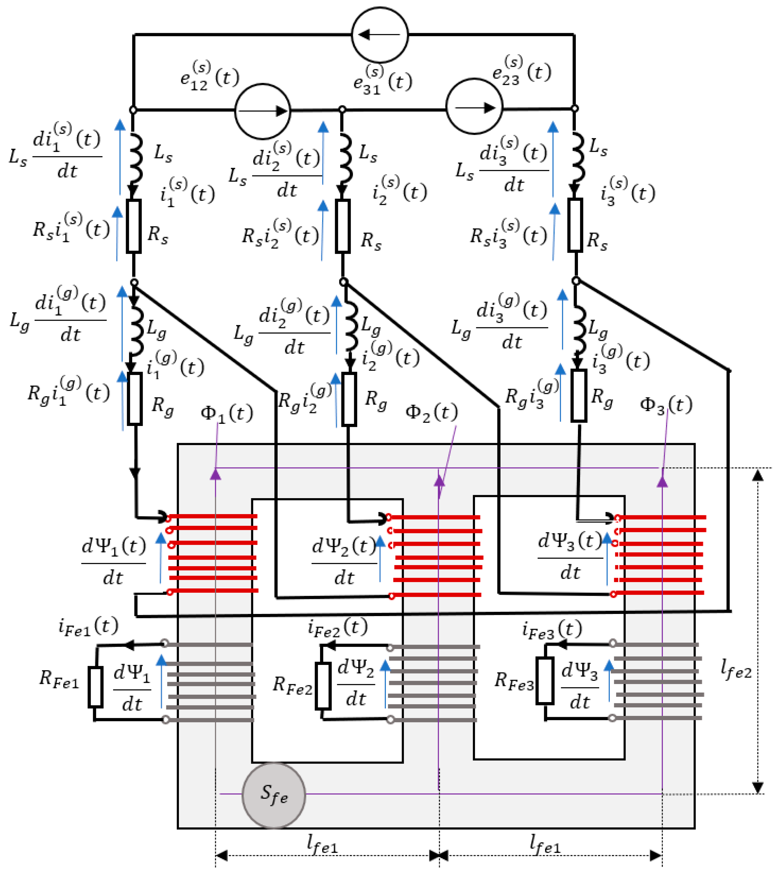
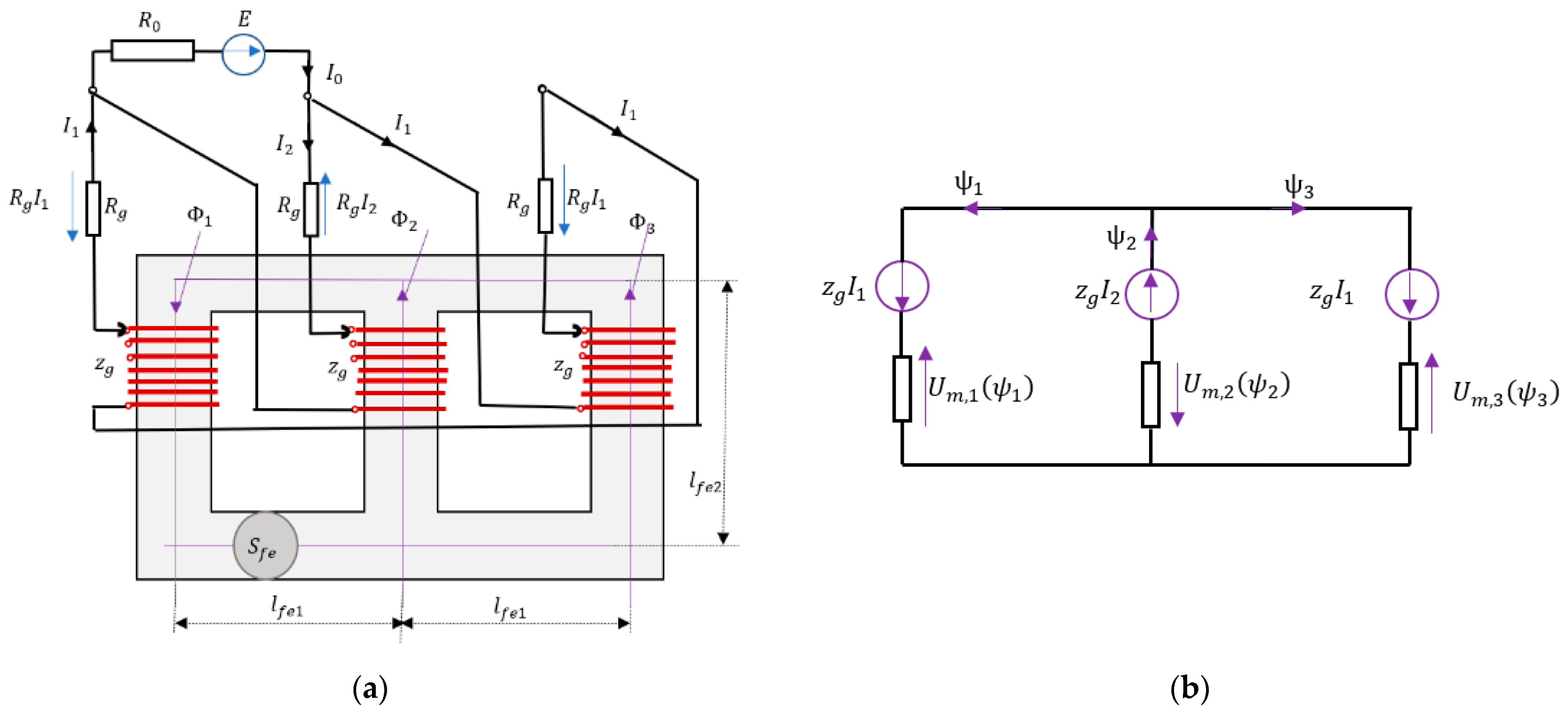
2.1. Model Concept

A research task of transient analysis was formulated for an unloaded three-phase transformer with primary side windings connected in delta. In order to carry it out, differential equations describing the adopted mathematical model were first formulated along with the assumptions.
The equivalent scheme of the transformer for the discussed model is shown in Figure 1, together with physical quantities that describe the model.
A list of all the designations used in this work can be found in Nomenclature.
For the planned calculation process, it was assumed that the switching on of the transformer at time instant t 0 had the effect of the emergence of three voltages with instantaneous values in the following form:
e 12 ( s ) ( t ) = E m 12 sin ω t + t 0 , e 23 ( s ) ( t ) = E m 23 sin ω t + t 0 + 2 3 π , e 31 ( s ) ( t ) = E m 31 sin ω t + t 0 + 4 3 π .
By making the parameter t 0 variable, it was possible to make the calculations dependent on the time instant specified in the waveform of the selected phase-to-phase voltage for the process of switching on the transformer, i.e., the start of the calculations.
In the investigation of the transient states, an invariant reference system was assumed. It was assumed that the reference point was the time instant at which the voltage e 12 ( s ) ( t ) passes through zero (which occurs for t = t 0 ).
We assume that the non-linear curve H ( B ) of the core material is known in the case of discussed transformer. In our experiment, this task was implemented using a polynomial described by odd powers (2). The correctness of this method was verified experimentally [3].
H ( B ) = k = 1 11 a k B 2 k 1
Restricting the model to include only the nonlinear relationship I 0 Ψ was insufficient for model losses in the ferromagnetic material of the core. The total losses were taken into account according to the classical concept of transformer modeling. In each column of the three-phase transformer, an additional electromotive force was introduced in the form of a flux linkage derivative d d t Ψ k ( t ) at the terminals of a coil with z g turns. The coil with zero internal resistance was loaded with a resistance R Fe , k , which modeled the total iron power losses in the k t h column of the transformer (Figure 1).
Using the circuit description in modeling the magnetic circuit of the transformer, we can state that:
d d t Ψ k ( t ) = R Fe , k i Fe , k ( t )
where i Fe , k ( t ) is a current of the coil under consideration.
It was assumed that the parameters R Fe , k could be determined by measuring the active power of a transformer operating at steady state under idling conditions.
The mathematical model of the transformer formulated in this way also offers the possibility of determining the steady state in the form of a limit cycle of the solution of the relevant differential equations. Details on the experimentally verified methodology of this subject may be found in [3,27].

2.2. Residual Magnetism

The formulated transformer model intentionally did not consider magnetic hysteresis. This was not necessary, since it was not intended to track the history of core magnetization, that is, the points at which reversals in the directions of changes in magnetic currents and fluxes occurred. Instead, the model offered the possibility of taking into account the magnetization of the transformer core at the particular time instant, when the transformer was switched on. The state of magnetization was taken into account in the model in the form of residual magnetism. If we know the amount of residual magnetism, then it is possible to set initial conditions for the state variables Ψ 2 ( t 0 ) , Ψ 3 ( t 0 ) , which represent flux linkages.
As indicated by numerous literature sources, e.g., [11,14], the energizing of unloaded transformer is accompanied by the occurrence of current pulses. Their presence is limited to the first period determined by the supply voltage. The amplitudes of these currents, as a rule, exceed the rated values, and not infrequently reach values close to short-circuit values.
Basing on these findings, we argue that if the transient state analysis of the transformer is limited to a single period from the energizing instant, the proposed model will make it possible (if initial conditions are set) to investigate the impact of residual magnetism on the magnitudes of generated current pulses.
The analysis of the physics of the formation of current pulses has already established that they (the pulses) first appear as a result of locating the working point of the inductor ( I 0 Ψ solution) far in the saturation region of transformer’s core magnetization curve [3,12].
Therefore, the inclusion of the core’s residual magnetism in the model must be supported by an accurate approximation of the core’s nonlinear curve in the saturation region.

2.3. Dynamic Equations of the Unloaded Transformer Dy

In the developed mathematical model of the transformer, the magnetomotive forces (mmfs) generated by the coil currents i k ( g ) ( t ) ( k = 1 , 2 , 3 ) were supplemented by the magnetomotive forces generated by certain equivalent currents i R Fe , k ( t ) . These mmfs are expressed as z g i R Fe , k ( t ) , and they corresponded to real power losses in the ferromagnetic core.
Such a concept for modeling a three-phase transformer with three columns and star-connected primary side windings has been comprehensively analyzed before, and the results of these studies were published in [27]. There, the flux linkages Ψ 1 ( t ) , Ψ 2 ( t ) were chosen as the state variables.
In the considered case, the windings of the primary side of the three-phase transformer were delta-connected. The flux linkages Ψ 2 ( t ) , Ψ 3 ( t ) were chosen as the state variables in the magnetic circuit equations.
Taking into account Kirchhoff’s first and second laws for the magnetic circuit of a three-phase transformer with three columns (Figure 1) and Equation (3) modeling the total iron losses, the equations of state for the variables Ψ 2 ( t ) , Ψ 3 ( t ) were formulated:
G d d t Ψ 2 ( t ) d d t Ψ 3 ( t ) = h 4 ( X ) h 5 ( X )
where G = 1 R Fe 1 + 1 R Fe 2 1 R Fe 1 1 R Fe 2 1 R Fe 3
and
h 4 ( X ) = i 1 ( g ) ( t ) + i 2 ( g ) ( t ) + 1 z g U m , 1 Ψ 2 ( t ) Ψ 3 ( t ) 1 z g U m , 2 Ψ 2 ( t ) h 5 ( X ) = i 2 ( g ) ( t ) + i 3 ( g ) ( t ) 1 z g U m , 2 Ψ 2 ( t ) + 1 z g U m , 3 Ψ 3 ( t )
When the system of Equation (4) is solved for the derivatives, the results are:
d d t x 4 ( t ) d d t x 5 ( t ) = d d t Ψ 2 ( t ) d d t Ψ 3 ( t ) = G 1 h 4 ( X ) h 5 ( X ) = f 4 ( X ) f 5 ( X )
where C = G 1 c 1 , 1 c 1 , 2 c 2 , 1 c 2 , 2
and c 1 , 1 = 1 1 R Fe 1 + 1 R Fe 2 + R Fe 3 R Fe 1 R Fe 2 c 1 , 2 = 1 1 R Fe 2 + 1 R Fe 3 + R Fe 1 R Fe 2 R Fe 3 c 2 , 1 = 1 1 R Fe 3 + 1 R Fe 1 + R Fe 2 R Fe 3 R Fe 1 c 2 , 2 = 1 1 R Fe 3 + 1 R Fe 1 + R Fe 2 .
Equations for three independent circulations appeared as a result of applying Kirchhoff’s second law to the modeled equivalent circuits of the primary side of the transformer (Figure 1):
L s d d t i 1 ( s ) ( t ) R s i 1 ( s ) ( t ) + L s d d t i 2 ( s ) ( t ) + R s i 2 ( s ) ( t ) + L g d d t i 2 ( g ) ( t ) + R g i 2 ( g ) ( t ) + + d d t Ψ 2 ( t ) = e 12 ( s ) ( t ) L s d d t i 2 ( s ) ( t ) R s i 2 ( s ) ( t ) + L s d d t i 3 ( s ) ( t ) + R s i 3 ( s ) ( t ) + L g d d t i 3 ( g ) ( t ) + R g i 3 ( g ) ( t ) + + d d t Ψ 3 ( t ) = e 23 ( s ) ( t ) L g d d t i 1 ( g ) ( t ) R g i 1 ( g ) ( t ) + L g d d t i 2 ( g ) ( t ) + R g i 2 ( g ) ( t ) + L g d d t i 3 ( g ) ( t ) + R g i 3 ( g ) ( t ) + + d d t Ψ 1 ( t ) + d d t Ψ 2 ( t ) + d d t Ψ 3 ( t ) = e 12 ( s ) ( t )
where
i 1 ( s ) = i 1 ( g ) i 2 ( g ) i 2 ( s ) = i 2 ( g ) i 3 ( g ) i 3 ( s ) = i 3 ( g ) i 1 ( g )
The resulting system of equations was ordered in matrix form:
L d d t i 1 ( g ) ( t ) d d t i 2 ( g ) ( t ) d d t i 3 ( g ) ( t ) = R i 1 ( g ) ( t ) i 2 ( g ) ( t ) i 3 ( g ) ( t ) d d t Ψ 2 ( t ) d d t Ψ 3 ( t ) 0 + e 12 ( s ) ( t ) e 12 ( s ) ( t ) 0
where
L = L s 2 L s + L g L s L s L s 2 L s + L g L g L g L g ,   R = R s 2 R s R g R s R s R s 2 R s R g R g R g R g
When the system of Equation (7) is solved for the derivatives, taking into account solution (5), the results are:
d d t x 1 ( t ) d d t x 2 ( t ) d d t x 3 ( t ) = d d t i 1 ( g ) ( t ) d d t i 2 ( g ) ( t ) d d t i 3 ( g ) ( t ) = f 1 ( X ) f 2 ( X ) f 3 ( X )
where
f 1 ( X ) f 2 ( X ) f 3 ( X ) = L 1 R i 1 ( g ) ( t ) i 2 ( g ) ( t ) i 3 ( g ) ( t ) + f 4 ( X ) + e 21 ( s ) ( t ) f 5 ( X ) + e 32 ( s ) ( t ) 0 f 1 ( X ) f 2 ( X ) f 3 ( X ) = L 1 R i 1 ( g ) ( t ) i 2 ( g ) ( t ) i 3 ( g ) ( t ) + L 1 f 4 ( X ) + e 21 ( s ) ( t ) f 5 ( X ) + e 32 ( s ) ( t ) 0
While the inverse matrix L−1 of matrix L assumes the following analytical form:
D = L 1 = 1 3 k + 1 L g 1 1 k + 1 1 0 k 0 1 k
The relationships formulated as differential Equations (5) and (8) form a general system of equations of state for an unloaded transformer.
The model formulated in this way does not take into account magnetic hysteresis. However, its simplifications (Section 6) make it possible to use it in the analysis of the influence of residual magnetism (and the parameter R Fe , k of the model) on the maximum values of the inrush currents of the unloaded transformer appearing during the first period determined by the supply voltage.

3. Investigation

The transformer data adopted in the test calculations are included in Appendix A.
Powercore® H 105-30 electrical steel was used in the experiment, which is manufactured by the ThyssenKrupp company. Material characteristics: density 7.65 kg/dm3, maximum specific loss at 1.7 T is 1.05 W/kg.

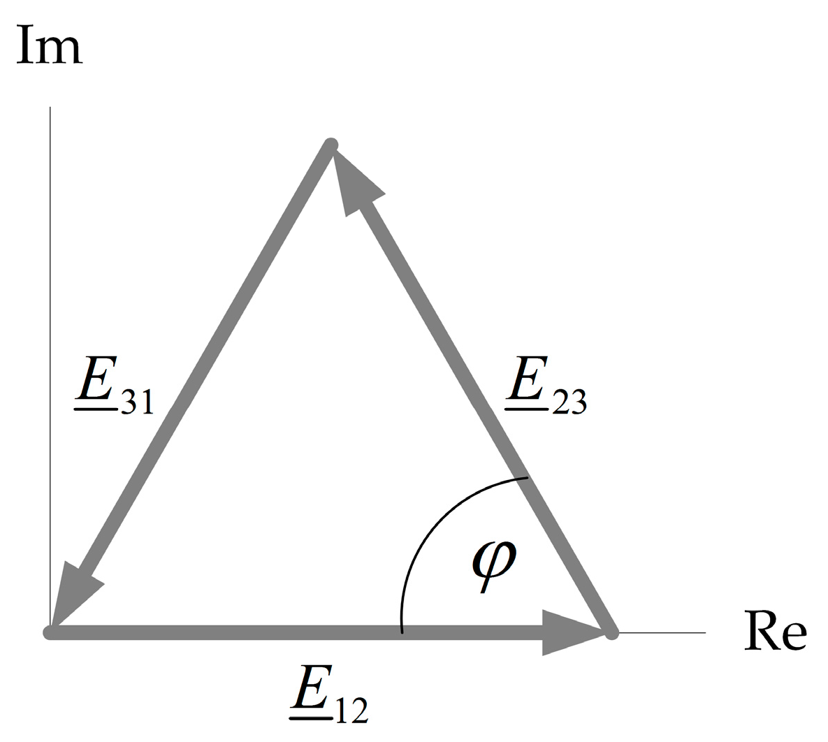
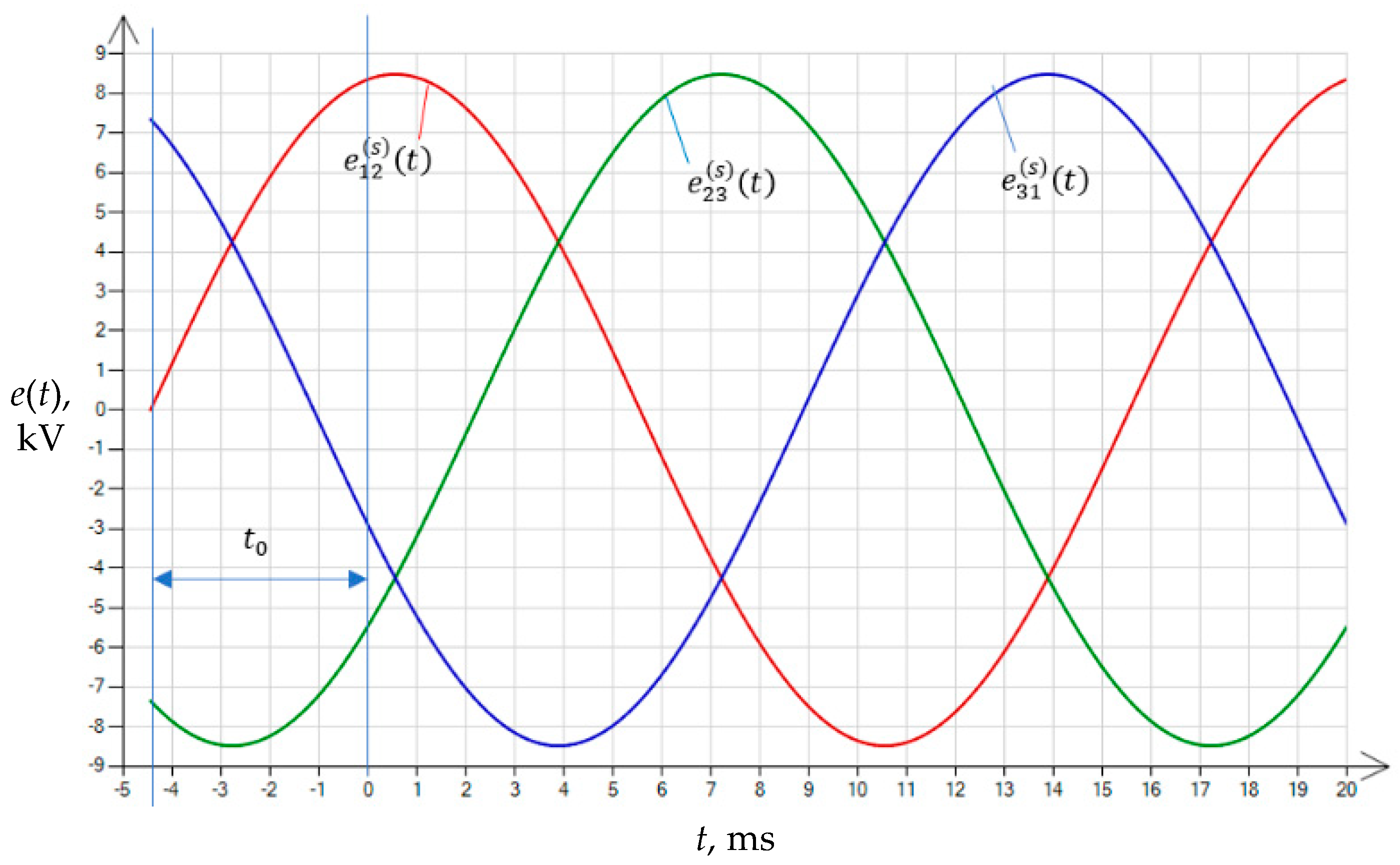
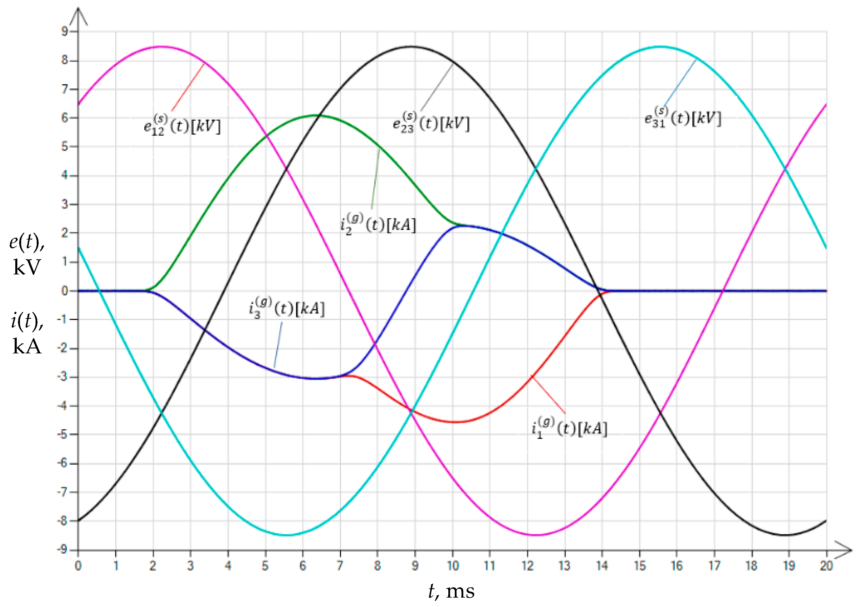
3.1. Definition of Supply Voltages Together with the Method That Takes into Account the Time Instant Determined (Set) in the Supply Voltage Waveform

To define the symmetrical supply voltages of the discussed transformer, it was assumed that they are sinusoidally alternating waveforms with pulsation ω = 2 π f and arbitrarily set rms values of phase-to-phase voltages, E 12 , E 23 , E 31 . It was also assumed that the initial phase angle for one (arbitrarily chosen) voltage was known. This was sufficient because the phase angles of other voltages were defined by the geometry of the triangle (Figure 2).
The complex rms value of the reference voltage E 12 assumed in the experiment was
E ¯ 12 = E 12
According to Figure 2, it was deduced that
E ¯ 23 = a + j k p h s q E 23 sin φ
where
a = E 23 cos φ = E 12 2 + E 23 2 + E 31 2 2 E 12 , φ = arccos a E 23 , k p h s q = 1 positive   phase   sequence 1 negative   phase   sequence
The introduced parameter k p h s q made it possible to take into account the effect of the phase sequence on the calculated waveforms of transformer inrush currents.
The defined rms complex values of sinusoidally variable phase-to-phase voltages E ¯ 12 , E ¯ 23 , E ¯ 31 constituted the basis for determining their instantaneous values in the form of the following functions:
e 12 ( s ) ( t ) = 2 E ¯ 12 sin ω t + t 0 + arg E ¯ 12 , e 23 ( s ) ( t ) = 2 E ¯ 23 sin ω t + t 0 + arg E ¯ 23 , e 31 ( s ) ( t ) = 2 E ¯ 31 sin ω t + t 0 + arg E ¯ 31 .
Functions (11), representing input phase-to-phase voltages at the terminals of the primary winding of an unloaded transformer, met the requirements of the construction of Equations of states (5) and (8). The parameter t 0 present in the formula made it possible to define the time instant specified in the voltage waveform at which the indicated voltage appeared at the given transformer winding.
Since the argument of the reference voltage considered in the experiment E ¯ 12 was assumed to be zero arg ( E ¯ 12 ) = 0 (Figure 2), its function e 12 ( s ) ( t ) took the form of
e 12 ( s ) ( t ) = 2 E ¯ 12 sin ω t + t 0
The investigation of the transient state of the unloaded transformer was possible via the analysis of the solutions of the systems of differential Equations (5) and (8). In these equations, the initial point of integration was assumed to be zero ( t 0 = 0 ). This meant that the starting point of the integral of the system of Equations (5) and (8) was t 0 away in time from the reference point determined by the passage of the voltage e 12 ( s ) ( t ) through zero (Figure 3).
The positive phase sequence e 12 ( s ) ( t ) , e 23 ( s ) ( t ) , e 31 ( s ) ( t ) shown in Figure 3 was taken into account in further calculations as a coefficient with the value k p h s q = 1 .
The presented method made it possible to set the parameter t 0 in the study of the effect of the time instant determined (defined) in the supply voltage waveform on the maximum values of the inrush current of the unloaded transformer in the first period determined by the supply voltage.

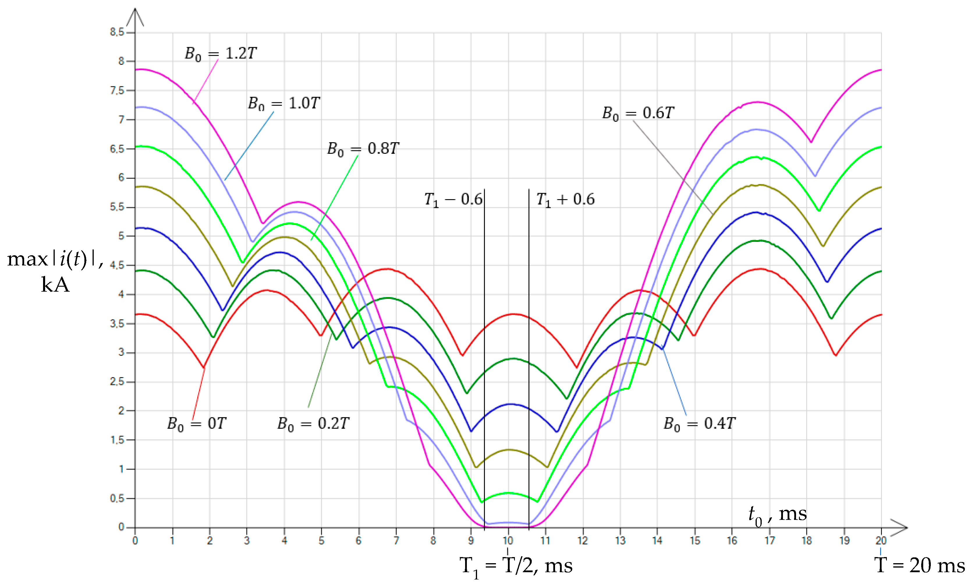
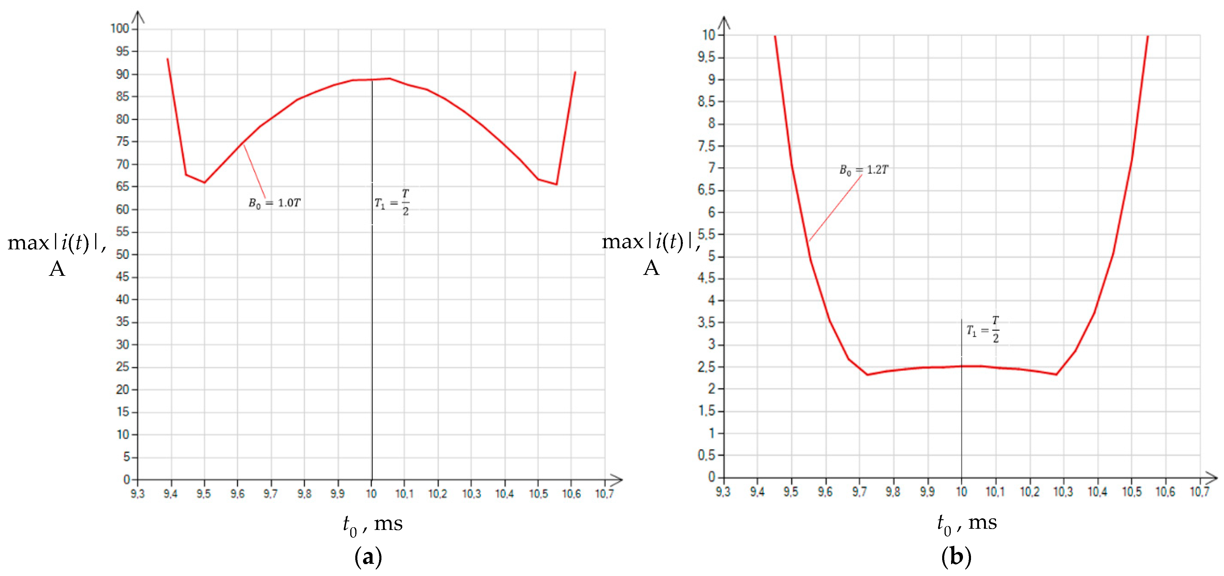
3.2. Study of the Influence of Residual Magnetism on the Maximum Values of Inrush Currents of an Unloaded Transformer

The study of the influence of residual magnetism on the maximum values of the current pulses accompanying the energizing of an unloaded transformer was carried out by setting initial conditions in the form of state variables
x 4 ( 0 ) = Ψ 2 ( 0 ) x 5 ( 0 ) = Ψ 3 ( 0 )
identical with flux linkages
x 4 ( 0 ) = Ψ 2 ( 0 ) = B 2 z g s Fe x 5 ( 0 ) = Ψ 3 ( 0 ) = B 3 z g s Fe
where B 2 , B 3 are the residual flux density of the transformer core columns, namely the center and outer columns (Figure 1).
For the purposes of the study, four scenarios (variants) were also established, with non-randomly selected sets of residual flux density values B 1 , B 2 , B 3 (Table 1) in successive columns of the transformer core. This procedure was carried out because of future applications, including the need to select the transformer core column whose winding will be supplied in the tests.
The remaining initial conditions of the system of Equations (5) and (8) were assumed to be zero in all calculation cycles x 1 ( 0 ) = i 1 ( g ) ( 0 ) ; x 2 ( 0 ) = i 2 ( g ) ( 0 ) ; x 3 ( 0 ) = i 3 ( g ) ( 0 ) .
The influence of the time instant determined in the waveform of the supply voltage applied to the transformer was investigated by changing the parameter t 0 in functions (11) applied then to the equations of states (5) and (8).

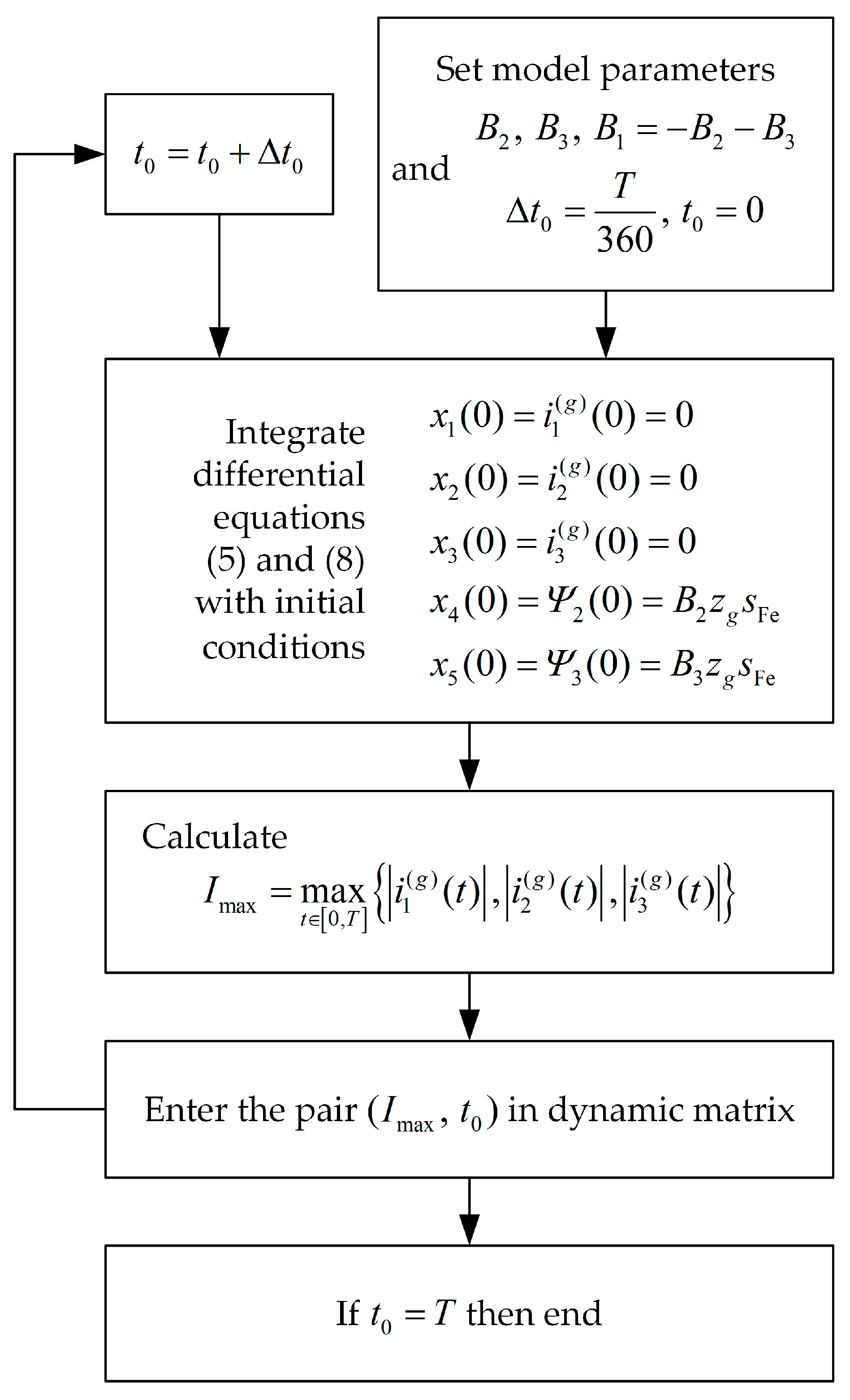
3.3. Implementation of Calculations—Calculation Algorithm

Figure 4 shows the flowchart of the algorithm applied in both tests. The algorithm was input into the authors’ own C# software [30]. The program allows the precise calculation and visualization of the distributions of the maximum values of the inrush currents of an unloaded transformer depending on the time instant t 0 characterizing the time instant in the waveform of the switched supply voltage and also the values and initial scenarios of the pre-magnetization of transformer’s different columns. To integrate the stiff differential Equations (5) and (8) of the transformer model, the authors’ own ninth-order Radau IIA method was used [31,32,33].

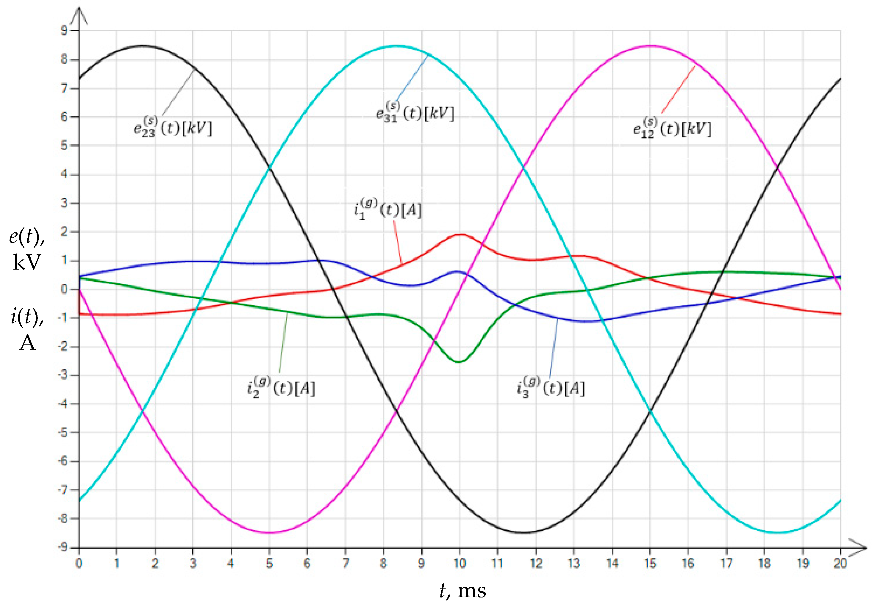
4. Simulation Results

Figure 5 shows the results of the analysis of the distribution of the maximum values of inrush currents of the unloaded transformer for four variants of the pre-magnetization of the core (Table 1) in a positive phase sequence system (Figure 3).
The conditions of the experiment in Figure 5 were used in its repeated implementation, in which the phase sequence was changed to the opposite sequence. The calculation results obtained under the conditions of such a modified power supply are shown in Figure 6.
A comparison of the results of the calculations presented in Figure 5 and Figure 6 showed that for the pre-magnetization scenario in the center column with a value twice that of the outermost columns (this refers to the absolute value), the distributions of maximum currents do not depend on the phase sequence.
For pre-magnetization scenarios 1 and 4 (Table 1), the calculations of inrush currents of the unloaded transformer led to results highly consistent with each other (similar shape and values of the obtained waveforms in Figure 5 and Figure 6).
In a further stage of the study, it was assumed that the initial magnetization of the transformer core would be carried out according to variant 1 (Table 1).
Figure 7 shows the result of the experiment of energizing the unloaded transformer for the residual magnetism set in variant 1 and for the set time instant t 0 = 2.77 ms specified in the waveform of the reference supply voltage e 12 ( s ) ( t ) .
The calculated maximum instantaneous value of the unloaded transformer inrush current during the first transient period was I m a x = max t 0 , T i 1 ( g ) ( t ) , i 2 ( g ) ( t ) , i 3 ( g ) ( t ) = 6 kA.
In the case of energizing the transformer after a time t 0 = 10 ms from the transition of voltage e 12 ( s ) ( t ) through zero, the maximum instantaneous value of the inrush current of the unloaded transformer during the first transient period was reduced to only I m a x = max t 0 , T i 1 ( g ) ( t ) , i 2 ( g ) ( t ) , i 3 ( g ) ( t ) = 2.5 A (Figure 8).

5. Algorithm for Selecting the Time Instant Specified in the Waveform of the Switched Supply Voltage

The results of the performed experiments and the diagnosed regularities of the model were used to develop an algorithm for selecting the time instant t 0 calculated from the reference point of the voltage e 12 ( s ) ( t ) transition through zero.
With regard to the selection of the supply voltage and the terminals of the primary side of the transformer to which this voltage is to be applied, it was determined that the most optimal configuration was provided by the computationally verified voltage e 12 ( s ) ( t ) and the terminals of the primary winding wound on the center column of the transformer (Figure 1), as seen in scenario 1.

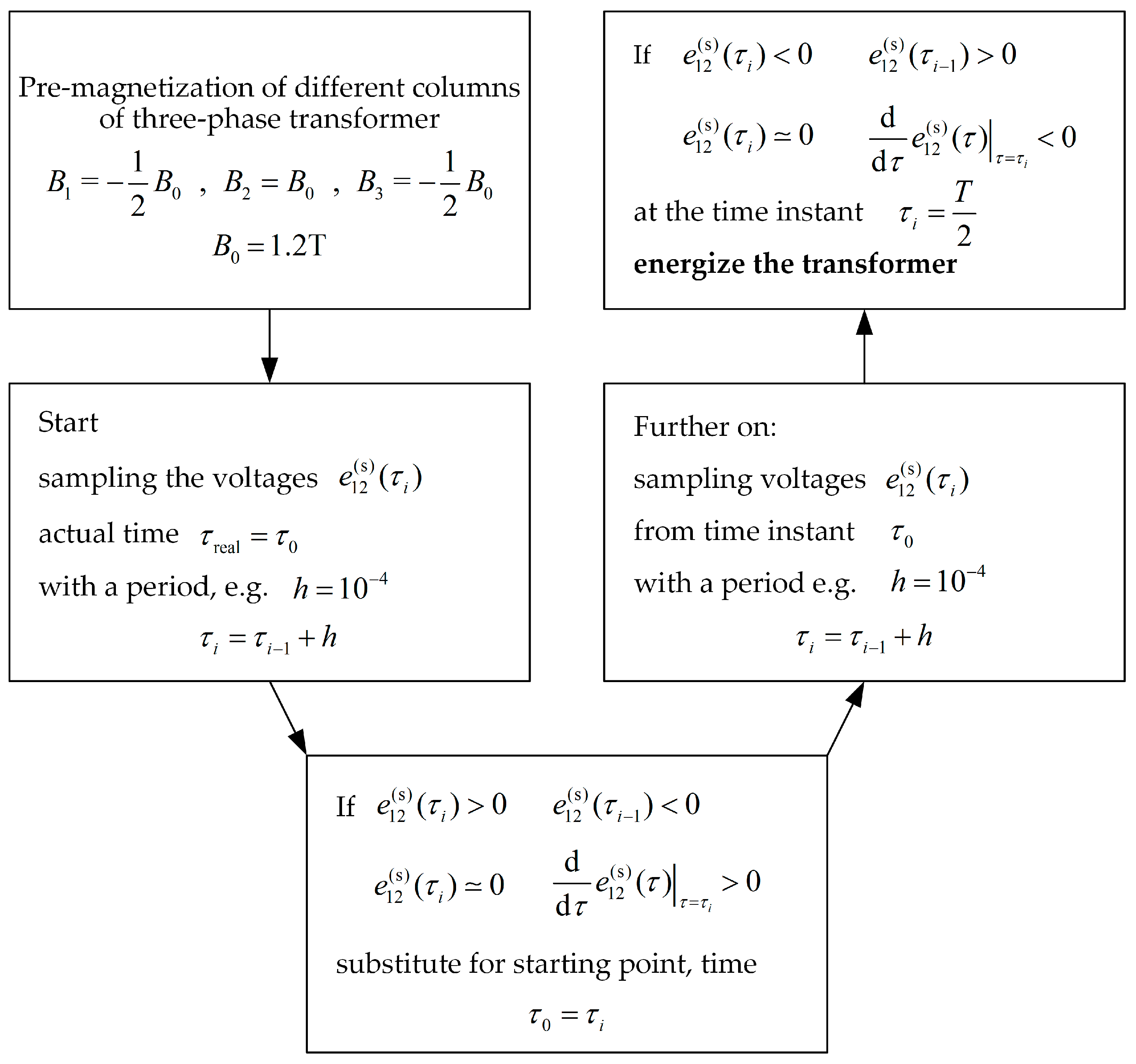
5.1. Method of Implementation of Pre-Magnetization of the Core Columns of the Tested Transformer

Due to the difficulties associated with measuring the residual magnetism of three-phase transformers [12,18], it was decided that the pre-magnetization technique of the core [27] instead of its measurement should be used. The schematic diagram of the solution involving the pre-magnetization of the core of an unloaded transformer with delta-connected primary side windings is presented in Figure 9a.
The concept of the pre-magnetization of the core of the transformer under study envisages the generation of a magnetization of twice the value and opposite polarity in the center column than is the case in the outermost columns (variant 1) (Figure 9b).
As shown in the conducted numerical experiments, such as the proportion and symmetry of the initial magnetization guarantees the distribution of the maximum values of the inrush current of the unloaded transformer as a function of the switching time calculated with respect to the transition of the voltage e 12 ( s ) ( t ) through zero and independent of the phase sequence of the supply voltages e 12 ( s ) ( t ) , e 23 ( s ) ( t ) , e 31 ( s ) ( t ) .

5.2. Selection of the Currents Required for Core Pre-Magnetization

The next step was to estimate what values of current are necessary for pre-magnetization in the system shown in Figure 9.
The starting point in the calculations was the value of the transformer winding resistance R g . Since the value of this resistance is relatively small, the condition for selecting the resistance R 0 in the circuit, as shown in Figure 9a, was formulated as [34]:
R 0 > > R g
It was possible to determine the DC currents flowing through the transformer windings without any problem via the following:
I 0 = E 0 R 0 , I 1 = 1 3 E 0 R 0 , I 0 = 2 3 E 0 R 0
The currents determined in this way for the different windings of the three-phase transformer allowed the formulation of a system of nonlinear equations based on magnetic circuit theory (Figure 9b). In the equations, magnetic voltage drops were taken into account with the omission of the dynamic term (i.e., the Formula [27]).
U m , k ( Ψ k ) = h Fe , k H Ψ k ( t ) z g s Fe , k = 1 , 2 , 3
The system of nonlinear equations determining the distribution of flux linkages took the following form:
f 1 ( X ) f 2 ( X ) f 3 ( X ) = I 0 z g U m , 1 ( x 1 ) U m , 2 ( x 2 ) I 0 z g U m , 2 ( x 2 ) U m , 3 ( x 3 ) x 1 + x 2 x 3 = 0
where X = x 1 , x 2 , x 3 T = Ψ 1 , Ψ 2 , Ψ 3 T .
The formulated system of equations was solved for the given values of current I 0 by relating the solutions of Ψ i ( i = 1 , 2 , 3 ) to the corresponding average values of magnetic flux density:
B i = Ψ i z g s Fe
The solution of the system of Equation (18), as shown in Equation (19), for different values of current I 0 is presented in Figure 10.
The calculated characteristic unambiguously proves that the proposed method of the pre-magnetization of the transformer core results in flux density levels in the different columns of the core according to variant 1:
B 2 = B 0 , B 1 = 1 2 B 0 , B 3 = 1 2 B 0
where B 0 depends on the magnetization current I 0 .
For the calculated magnetization configuration (20), the opposite magnetization can also be considered. To obtain this configuration, it is enough to change the direction of current flow I 0 in the circuit shown in Figure 9a.
Turning off the flow of current I 0 in the pre-magnetization system will reduce the value of flux density in the different columns of the core. For transformer sheets (soft magnetic materials), the value of flux density B 0 will correspond to the value of remanence B r , which is significantly lower than saturation flux density (by as much as 50%).
In the test data adapted for the simulation, it was assumed that the transformer sheet has a saturation flux density of 1.9 T. Hence, the value of the flux density B 0 , representing the initial magnetization of the core in the calculations in variant (20), will vary up to a value of 1.2 T.
Results of the calculations of the maximum values of inrush currents
I m a x ( t 0 ) = max t 0 , T i 1 ( g ) ( t ) , i 2 ( g ) ( t ) , i 3 ( g ) ( t )
of the unloaded transformer in the first period of the transient state from the energization, depending on the adopted value of B 0 , are presented in Figure 11.
The calculated inrush currents are functions dependent on time t 0 (the time instant of switching on) calculated with respect to the transition of voltage e 12 ( s ) ( t ) through zero with positive derivative at the point d d t e 12 ( s ) ( t ) > 0 (Figure 12).
The results were obtained for the initial magnetization, as seen in (20), enforced according to the scheme in Figure 9 with a positive phase sequence of supply voltage.
The analysis of the effect of the value of B 0 on the distribution of the maximum values of inrush currents showed the existence of an interval of the variability of the maximum values of the currents, in which the maximum values of the currents decrease as the flux density B 0 increases.
It was found that in the interval t 0 1 2 T 0.6 m s , 1 2 T + 0.6 m s for B 0 = 1.0 T, the maximum inrush currents reached values in the order of tens of amperes, while for B 0 = 1.2 T, the values decreased to a few amperes (Figure 13).
Outside the indicated time interval, the opposite phenomenon was observed: the increase in B 0 was accompanied by a sharp increase in the maximum values of inrush currents. For t 0 = 0 , the currents reached the highest possible values (kiloamperes) (Figure 11).
This means that in order to eliminate the large inrush currents accompanying the energizing of an unloaded three-phase transformer, its switching should be performed after a time t 0 = T 2 , calculated with respect to the reference point determined by the transition of the reference voltage (here: e 12 ( s ) ( t ) ) through zero with a positive derivative at the point d d t e 12 ( s ) ( t ) > 0 (Figure 12).
At the energizing time instant t 0 = T 2 , the instantaneous voltage e 12 ( s ) ( t ) = 0, while its derivative is negative ( d d t e 12 ( s ) ( t ) < 0 ) (Figure 12).
The obtained solution is general and can be applied to any transformer, where primary winding is delta-connected and where columns are pre-magnetized according to (20) for B 0 > 1 T. The supply voltages e 12 ( s ) ( t ) , e 23 ( s ) ( t ) , e 31 ( s ) ( t ) can be arranged into a positive or negative phase sequence (without affecting the outcome).
The collected data can be used to construct a special device that will execute energizing the transformer at specific time instants in the supply voltage waveforms (Table 2).

5.3. The Strategy of Energizing a Three-Phase, Three-Column Transformer Where Primary Winding Is Delta-Connected and Where the Columns Are Pre-Magnetized According to (20) at Specific Time Instants in the Supply Voltage Waveforms

The developed strategy is illustrated by the flowchart in Figure 14.

6. The Simplifications Implied by Using the Model Formulated in this Paper

  • The initial magnetization state of the transformer core can be taken into account as residual magnetism in the form of (assignable) initial conditions for the state variables Ψ 2 ( t 0 ) , Ψ 3 ( t 0 ) , which are essentially flux linkages Ψ 2 ( t 0 ) = B 2 z g s Fe and Ψ 3 ( t 0 ) = B 3 z g s Fe , where B 2 , B 3 is the residual flux density in the different columns of the transformer core.
  • The integration of the equations with the initial conditions formulated in this way leads in the first instance to a solution ( I 0 Ψ ) located deep in the saturation region of the ferromagnetic core curve; the maximum inrush currents of the unloaded transformer determined from this solution are calculated accurately.
  • Taking any initial conditions (e.g., zero) for the systems of Equations (5) and (8) as the starting point leads to a steady-state solution, which is the limit cycle of the transient state solution; the trajectories of the transition to this limit cycle have no physical interpretation in this case, since the assumed mathematical model does not take into account magnetic hysteresis (it does not track the history of core magnetization).
  • The model is suitable for the study of steady-state conditions of the transformer when the resistances R Fe , k are determined based on the idling losses, in which eddy currents and magnetic hysteresis are taken into account.
  • The completed tests have shown that there is no significant influence* of the parameter R Fe , k of the model on the maximum values of the inrush currents of the unloaded transformer in the first period of the transient state caused by energizing the transformer (*—lossiness values provided by the manufacturer of the transformer plates vary within wide limits).
Therefore, the developed model can be successfully used to study both the steady-state operation of a three-phase transformer (Dy) and to calculate the inrush currents that characterize it when it is energized under unloaded conditions.

7. Conclusions

The research task of modeling the dynamics of an unloaded three-phase transformer with a Dy connection group during the first transient period has been achieved.
The methodology and simulation results given in the article provide practical tools for studying the inrush currents of these devices.
What is particularly interesting, the developed model makes it possible to take into account the influence of residual magnetism in the different columns of the core and the time instant determined in the voltage waveform where the indicated voltage is supplied to the given winding of the transformer.
The completed calculations proved that for each scenario of core pre-magnetization of the modeled device, there is a time interval in which the energizing of an unloaded transformer is not accompanied by the occurrence of inrush current surges.
The tests showed that the width of such a time interval is more than 1 ms, and the currents occurring are several times higher than transformer’s steady-state idle current.
The remaining time intervals of the first period of the transient state caused by energizing an unloaded transformer should be associated with the occurrence of large current pulses.
For a three-phase transformer with connection group Dy, the initial magnetization of the core in the form of the variant specified in (20) is the easiest to implement in the circuit shown in Figure 9.
Such an arrangement allows the symmetric and proportional magnetization of the core of a three-column transformer. One of these columns, e.g., the center one, is twice as highly magnetized as the remaining columns; moreover, the magnetization is of opposite polarity.
The symmetry and adequate distribution of core magnetization, which are demonstrated in this paper, result in the fact that the positioning of the time interval (measured relative to a reference point determined by the transition of voltage e 12 ( s ) ( t ) through zero), during which the energizing of transformer is accompanied by a strong limitation of current pulses, does not depend on the phase sequence of phase-to-phase (line) voltages e 12 ( s ) ( t ) , e 23 ( s ) ( t ) , e 31 ( s ) ( t ) .
If the guidelines set out in this paper for a three-phase, three-column transformer are met, i.e., its core is pre-magnetized in a variant of (20) and it is switched on after time t 0 = T 2 is calculated from the instant when voltage e 12 ( s ) ( t ) passes through zero, the values of inrush currents in the first transient period will be minimal.
The next stage of the authors’ work will cover the experimental verification of the developed mathematical model, as well as the construction and testing of a device for the controlled switching of the supply voltage with the pre-magnetization of the transformer’s core.

Author Contributions

Conceptualization, M.Ł., B.B. and Ł.M.; Methodology, B.B. and Ł.M.; Software, B.B. and J.K.-P.; Validation, J.K.-P.; Formal analysis, M.Ł., J.K.-P. and Ł.M.; Investigation, B.B., J.K.-P. and Ł.M.; Data curation, J.K.-P.; Writing—original draft, B.B.; Writing—review & editing, M.Ł. and Ł.M.; Visualization, B.B. and Ł.M.; Supervision, M.Ł. and Ł.M.; Project administration, M.Ł.; Funding acquisition, M.Ł. All authors have read and agreed to the published version of the manuscript.

Funding

This research received no external funding.

Data Availability Statement

Data available on request from the authors.

Conflicts of Interest

The authors declare no conflict of interest.

Nomenclature

The list of symbols and notations used in this paper:
esinusoidal supply voltage
Ψkflux linkage associated with the transformer’s primary coil, computed as Ψk(t) = zgΦk(t), in the k th column of the transformer
ik(g)transformer primary current
RFe,kequivalent resistance representing the iron core losses
iFe,kactive component of the transformer’s idle current
Rsequivalent resistance of the power grid (power source)
Lsequivalent inductance (reactance) of the power grid (power source)
Rgprimary winding resistance
Lgleakage inductance of the primary winding
Hmagnetic field strength
Φmain flux leakage (effective value of the flux)
Bkflux density
sFecross-sectional area of the core of the transformer
zgnumber of turns in the primary windings
φ0phase of the initial supplied voltage
ωpulse

Appendix A

Table A1. Assumed data of the modeled transformer.
Quantity, UnitValue
Primary voltage PRI/phase to phase, V6000
Secondary voltage SEC/phase to phase, V230
Frequency50
Rated primary current, A800
Number of primary winding turns, N160
Iron power loss (for 1.7 T), W/kg1.05
Copper power loss, kW50
Short-circuit voltage, %5
Core cross-sections, m20.110565
Column length, m2
Length of the yoke, m0.76
Equivalent resistance of the network, Ω0.1
Equivalent reactance of the network, Ω0.2
Table A2. Function H(B) coefficients obtained from solving the estimation problem based on the manufacturer’s data.
k a k
129.9624271037522
2−76.4912078883278
3420.867774746849
4−1274.37623231261
52196.27285444425
6−2301.93260519503
71516.77585894405
8−630.577358829122
9160.397849549712
10−22.7840824031901
111.38472183966324

References

  1. CIGRÉ Working Group. C4.307. Transformer Energization in Power Systems: A Study Guide, 568th ed.; CIGRÉ Publication: Paris, France, 2014; pp. 8–73. [Google Scholar]
  2. Kulkarn, S.V.; Khaparde, S.A. Transformer Engineering: Design, Technology, and Diagnostics, 2nd ed.; Taylor & Francis Inc.: Boca Raton, FL, USA, 2012; pp. 1–750. [Google Scholar]
  3. Majka, Ł.; Baron, B.; Zydroń, P. Measurement-based stiff equation methodology for single phase transformer inrush current computations. Energies 2022, 15, 7651. [Google Scholar] [CrossRef]
  4. Barros, R.M.R.; da Costa, E.G.; Araujo, J.F.; de Andrade, F.L.M.; Ferreira, T.V. Contribution of inrush current to mechanical failure of power transformers windings. High Volt. 2019, 4, 300–307. [Google Scholar] [CrossRef]
  5. Steurer, M.; Frohlich, K. The impact of inrush currents on the mechanical stress of high voltage power transformer coils. IEEE Trans. Power Deliv. 2002, 17, 155–160. [Google Scholar] [CrossRef]
  6. Pandey, S.B.; Lin, C. Estimation for a life model of transformer insulation under combined electrical and thermal stress. IEEE Trans. Reliab. 1992, 41, 466–468. [Google Scholar] [CrossRef]
  7. Alassi, A.; Ahmed, K.H.; Egea-Alvarez, A.; Foote, C. Transformer Inrush Current Mitigation Techniques for Grid-Forming Inverters Dominated Grids. IEEE Trans. Power Deliv. 2023, 38, 1610–1620. [Google Scholar] [CrossRef]
  8. Hamilton, R. Analysis of transformer inrush current and comparison of harmonic restraint methods in transformer protection. IEEE Trans. Ind. Appl. 2013, 49, 1890–1899. [Google Scholar] [CrossRef]
  9. Ni, R.; Wang, P.; Moxley, R.; Flemming, S.; Schneider, S. False Trips on Transformer Inrush-Avoiding the Unavoidable. In Proceedings of the 68th Annual Conference for Protective Relay Engineers, College Station, TX, USA, 30 March–2 April 2015. [Google Scholar]
  10. Nagpal, M.; Martinich, T.G.; Moshref, A.; Morison, K.; Kundur, P.P. Assessing and limiting impact of transformer inrush current on power quality. IEEE Trans. Power Deliv. 2006, 21, 890–896. [Google Scholar] [CrossRef]
  11. Blume, L.F.; Camilli, G.; Farnham, S.B.; Peterson, H.A. Transformer magnetizing inrush currents and influence on system operation. Trans. Am. Inst. Electr. Eng. 1944, 63, 366–375. [Google Scholar] [CrossRef]
  12. Horiszny, J. Analysis and Reduction of Transformer Inrush Current; Gdansk University of Technology: Gdańsk, Poland, 2016; p. monograph 159. (In Polish) [Google Scholar]
  13. Chiesa, N.; Mork, B.A.; Høidalen, H.K. Transformer model for inrush current calculations: Simulations, measurements and sensitivity analysis. IEEE Trans. Power Deliv. 2010, 25, 2599–2608. [Google Scholar] [CrossRef]
  14. Brunke, J.H.; Frohlich, K.J. Elimination of transformer inrush currents by controlled switching. Part I. Theoretical considerations. IEEE Trans. Power Deliv. 2001, 16, 276–280. [Google Scholar] [CrossRef]
  15. Leite, J.V.; Benabou, A.; Sadowski, N. Transformer Inrush Currents Taking into Account Vector Hysteresis. IEEE Trans. Magn. 2010, 46, 3237–3240. [Google Scholar] [CrossRef]
  16. Cui, Y.; Abdulsalam, S.G.; Chen, S.; Xu, W. A sequential phase energization technique for transformer inrush current reduction. Part I: Simulation and experimental results. IEEE Trans. Power Del. 2005, 20, 943–949. [Google Scholar] [CrossRef]
  17. Chraygane, M.; El Ghazal, N.; Fadel, M.; Bahani, B.; Belhaiba, A.; Ferfra, M.; Bassoui, M. Improved modeling of new three-phase high voltage transformer with magnetic shunts. Arch. Electr. Eng. 2015, 64, 157–172. [Google Scholar] [CrossRef]
  18. Horiszny, J. Research of leakage magnetic field in deenergized transformer. Compel-Int. J. Comput. Math. Electr. Electron. Eng. 2018, 37, 1657–1667. [Google Scholar] [CrossRef]
  19. Mitra, J.; Xu, X.; Benidris, M. Reduction of three-phase transformer inrush currents using controlled switching. IEEE Trans. Ind. Appl. 2020, 56, 890–897. [Google Scholar] [CrossRef]
  20. Ni, H.; Fang, S.; Lin, H. A simplified phase-controlled switching strategy for inrush current reduction. IEEE Trans. Power Del. 2021, 36, 215–222. [Google Scholar] [CrossRef]
  21. Cano-González, R.; Bachiller-Soler, A.; Rosendo-Macías, J.A.; Álvarez-Cordero, G. Inrush current mitigation in three-phase transformers with isolated neutral. Electr. Power Syst. Res. 2015, 121, 14–19. [Google Scholar] [CrossRef]
  22. Nicolet, A.; Delince, F. Implicit Runge–Kutta methods for transient magnetic field computation. IEEE Trans. Magn. 1996, 32, 1405–1408. [Google Scholar] [CrossRef]
  23. Noda, T.; Takenaka, K.; Inoue, T. Numerical integration by the 2-stage diagonally implicit Runge–Kutta method for electromagnetic transient simulations. IEEE Trans. Power Del. 2009, 24, 390–399. [Google Scholar] [CrossRef]
  24. Pries, J.; Hoffmann, H. State Algorithms for Nonlinear Time-Periodic Magnetic Diffusion Problems Using Diagonally Implicit Runge–Kutta Methods. Magn. IEEE Trans. 2015, 51, 7208612. [Google Scholar] [CrossRef]
  25. Sowa, M. Ferromagnetic coil frequency response and dynamics modeling with fractional elements. Electr. Eng. 2021, 103, 1737–1752. [Google Scholar] [CrossRef]
  26. Sowa, M.; Majka, Ł.; Wajda, K. Excitation system voltage regulator modeling with the use of fractional calculus. AEU-Int. J. Electron. Commun. 2023, 159, 154471. [Google Scholar] [CrossRef]
  27. Baron, B.; Kolańska-Płuska, J.; Lukaniszyn, M.; Spałek, D.; Kraszewski, T. Solution of nonlinear stiff differential equations for a three-phase no-load transformer using a Runge-Kutta implicit method. Arch. Electr. Eng. 2022, 71, 1081–1106. [Google Scholar]
  28. Baron, B.; Kolańska-Płuska, J.; Waindok, A.; Kraszewski, T.; Kawala-Sterniuk, A. Application of Runge–Kutta implicit methods for solving stiff non-linear differential equations of a single-phase transformer model in the no-load state. Innovation Management and information Technology impact on Global Economy in the Era of Pandemic. In Proceedings of the 37th International Business Information Management Association Conference (IBIMA), Cordoba, Spain, 1–2 April 2021; pp. 8071–8087. [Google Scholar]
  29. Baron, B.; Kolańska-Płuska, J.; Kraszewski, T. Application of Runge–Kutta implicit methods to solve the rigid differential equations of a single-phase idle transformer model. Pozn. Univ. Technol. Acad. J. Electr. Eng. 2019, 100, 75–86. (In Polish) [Google Scholar]
  30. Baron, B.; Kolańska-Płuska, J. Numerical Methods of Solving Ordinary Differential Equations in C#; Politechnika Opolska Publisher: Opole, Poland, 2015. (In Polish) [Google Scholar]
  31. Hairer, E.; Wanner, G. Solving Ordinary Differential Equations II: Stiff and Differential-Algebraic Problems, 2nd ed.; Springer: Berlin/Heidelberg, Germany, 2010. [Google Scholar]
  32. Dekker, K.; Verwer, J.G. Stability of Runge–Kutta Methods for Stiff Nonlinear Differential Equations; North-Holland: Amsterdam, The Netherlands; New York, NY, USA; Oxford, UK, 1984. [Google Scholar]
  33. Dos Passos, W. Numerical Methods Algorithms and Tools in C#; CRC Press, Taylor & Francis Group LLC: Boca Raton, FL, USA; London, UK; New York, NY, USA, 2010; ebook-PDF; Available online: https://vdocuments.mx/numerical-methods-algorithms-and-tools-in-c-586e04e116cbc.html?page=1 (accessed on 11 April 2023).
  34. Majka, Ł.; Szuster, D. Application of the stationary DC decay test to industrial turbogenerator model parameter estimation. Przegląd Elektrotechniczny 2014, 90, 242–245. [Google Scholar]
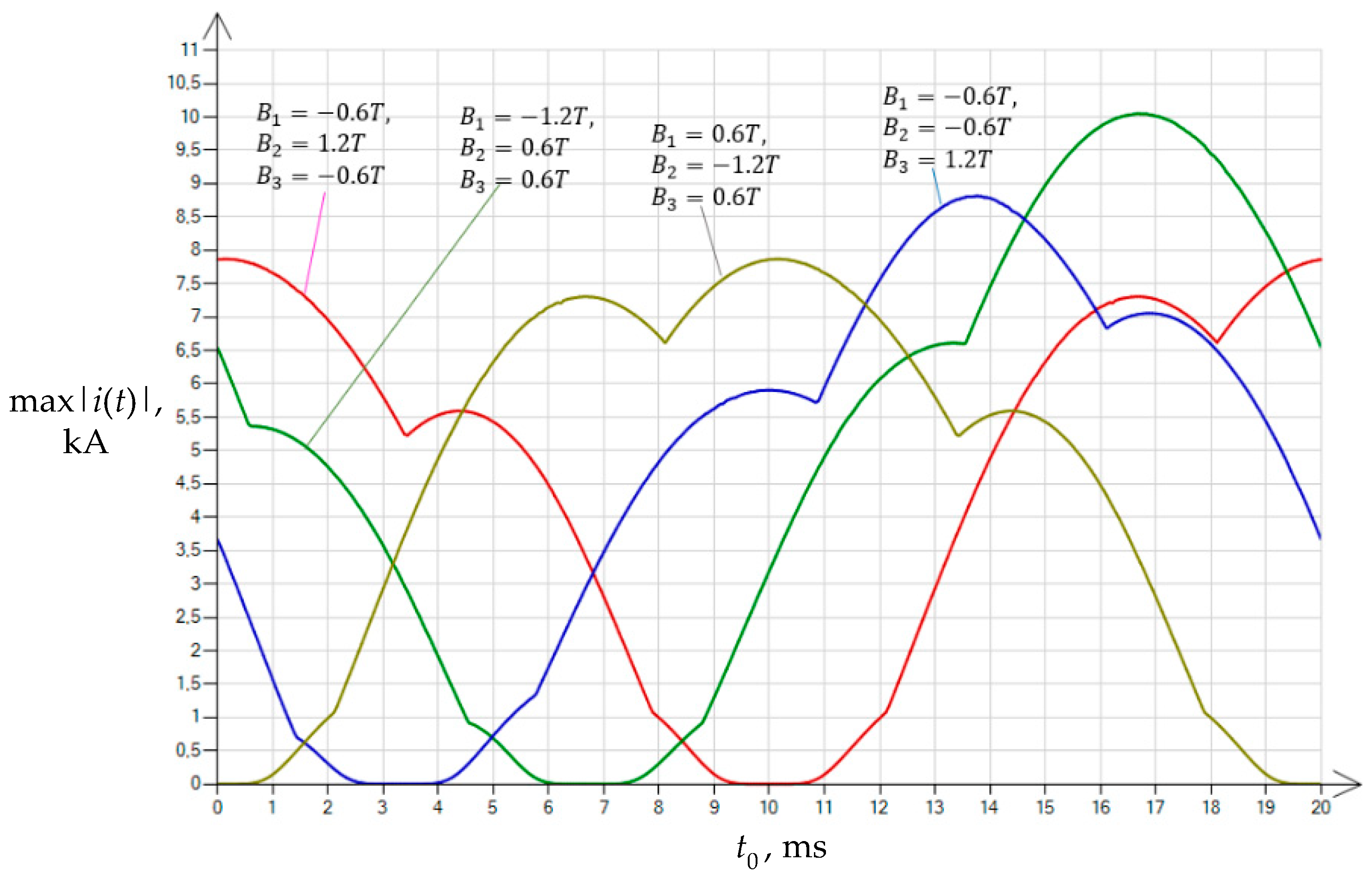
Figure 1. Equivalent scheme of the analyzed three-phase Dy transformer in no-load conditions.
Energies 16 05238 g001
Figure 2. Phasor diagram of supply voltages.
Energies 16 05238 g002
Figure 3. Visualization of how the t 0 parameter is set; the t 0 is the time shift from the reference point: the time instant when e 12 ( s ) ( t ) voltage passes through zero.
Energies 16 05238 g003
Figure 4. Structure of the computational algorithm examining the effect of the level of residual magnetism in the core and the time instant set in the supply voltage waveform on the maximum values of inrush currents of the unloaded transformer.
Energies 16 05238 g004
Figure 5. Distribution of the values of the maximum inrush currents of the unloaded transformer for the four variants of pre-magnetization, depending on the time instant t 0 , characterizing the time instant of energizing in the course of the supply voltage for the positive phase sequence.
Energies 16 05238 g005
Figure 6. Distribution of the values of the maximum inrush currents of the unloaded transformer for four variants of pre-magnetization, depending on the moment t 0 , identifying the time instant of energizing in the course of the supply voltage in the voltage for the negative phase sequence.
Energies 16 05238 g006
Figure 7. The waveforms of inrush currents of the unloaded transformer in the first period of the transient state; energizing occurred with residual magnetism present (variant 1) and at the time instant t 0 = 2.77 ms, defined in the waveform of the reference supply voltage e 12 ( s ) ( t ) .
Energies 16 05238 g007
Figure 8. The waveforms of the inrush currents of the unloaded transformer in the first period of the transient state; energizing occurred with residual magnetism present (variant 1) and at the time instant t 0 = 10 ms, defined in the waveform of the reference supply voltage e 12 ( s ) ( t ) .
Energies 16 05238 g008
Figure 9. Schematic diagram of the method of the pre-magnetization of the core of an unloaded transformer with delta-connected primary side windings (a) and an equivalent diagram of the magnetic circuit exhibiting forced flux distribution (b).
Energies 16 05238 g009
Figure 10. Dependence of magnetic flux density in different columns on magnetization current I 0 .
Energies 16 05238 g010
Figure 11. Distribution of maximum inrush currents of the unloaded transformer for seven variants of pre-magnetization B 0 , depending on the time instant t 0 , defined in the voltage waveform e 12 ( s ) ( t ) (as in Figure 12), and on the pre-magnetization of the core in configuration (20) for a positive phase sequence of supply voltage.
Energies 16 05238 g011
Figure 12. Visualization of the time instant of voltage switching on the transformer measured relative to the time instant when the voltage e 12 ( s ) ( t ) passes through zero, for a positive phase sequence of supply voltage.
Energies 16 05238 g012
Figure 13. Distribution of the maximum inrush currents of the unloaded transformer for two values of pre-magnetization B 0 = 1.0 T (a) and B 0 = 1.2 T (b), depending on the time instant t 0 1 2 T 0.6 m s , 1 2 T + 0.6 m s , defined in the waveform of the switched voltage e 12 ( s ) ( t ) , and on the pre-magnetization of the core in configuration (20).
Energies 16 05238 g013
Figure 14. Inrush current reduction strategy when energizing a three-phase transformer with delta-connected primary side windings requiring the pre-magnetization of the core columns.
Energies 16 05238 g014
Table 1. Test sets of values (variants) of pre-magnetization in each column of the transformer core.
Variant B 1 , T B 2 , T B 3 , T
1−0.61.2−0.6
2−1.20.60.6
3−0.6−0.61.2
40.6−1.20.6
Table 2. Switching conditions of the unloaded transformer for which the minimum values of inrush currents are obtained, taking into account the pre-magnetization in configuration (20).
Type k p h s q e 12 ( s ) ( t 0 ) d d t e 12 ( s ) ( t ) | t = t 0 t 0 e 12 ( s ) ( 0 ) d d t e 12 ( s ) ( t ) | t = 0
1−10 > 0 1 2 T 0 < 0
210 > 0 1 2 T 0 < 0
Disclaimer/Publisher’s Note: The statements, opinions and data contained in all publications are solely those of the individual author(s) and contributor(s) and not of MDPI and/or the editor(s). MDPI and/or the editor(s) disclaim responsibility for any injury to people or property resulting from any ideas, methods, instructions or products referred to in the content.

