Abstract
As an important electrical connection component in electrical equipment, the strap contact is directly related to the long-term operation stability of equipment. The electrical contact resistance (ECR) of the electrical connection structure is an important indicator for evaluating the reliability of the electrical contact system. In this research, the theoretical calculation of ECR of the strap contacts used by the G-W theoretical model and the fractal theoretical model is improved and compared. After comparison with the experimental measurement values, the rationality and accuracy of the two theoretical models are discussed. The results show that when the load is small (1–3 N), the maximum error of G-W model is 41%, while the fractal model method has a maximum error of 9%. When the load is large (4–10 N), the results of the two are almost the same, and the errors are both within 14%. In summary, the error range of the fractal model is smaller and the change trend is closer to the experimental value, which is suitable for a relatively better ECR analytical calculation theory. The research results can provide a theoretical basis for research on the electrical contact performance of the electrical contact structure of electrical equipment.
1. Introduction
With the gradual increases in the transmission capacity and years of operation of equipment, bushing overheating and discharge faults caused by electrical connection structure failures frequently occur, which seriously threatens the stability of a power system [1,2]. The electrical connection structure consists of a concentric central conductor and strap contacts, and the latter ensures the electrical connection when the other two have relative movement. As an essential part of the conductive structure, strap contacts need to withstand appropriate pressure to ensure good mechanical and electrical contact [3]. However, the uneven force caused by relative movement will lead to a change of the electrical contact resistance (ECR) of the strap contacts, causing partial overheating and bushing failure. According to engineering needs, it is urgent to study the generation, change mechanism, and trend of the ECR in the contact area.
The ECR comes from conductive spots generated after energization between rough contact surfaces. R. Holm initially studied conductive spots in a semi-infinite space, but he did not involve the interaction between the points [4]. Greenwood and Williamson et al. proposed a statistical analysis-based elastic contact model for rough surfaces (G-W model) and considered that the surface asperities only underwent elastic deformation [5,6]. The G-W model further was refined by Bush, Gibson, and Thomas (BGT) (1975) [7], The BGT model was further improved by McCool (1986) [8], Greenwood (2006) [9], and Carbone et al. [10]. The BGT model modeled the Hertzian contacts as elliptic contacts and predicted a perfectly linear relation between the true contact area and the applied load in the asymptotic limit of large separation for the first time [8]. The original G-W theory did not take into account the effect of summit heights on their mean curvature. To correct for this, Carbone proposed a very simple minimally corrected version of the G-W model [10]. An extensive survey of statistical models of rough surfaces was made by Persson et al. [11] which solves the problem that the standard maximum surface height parameters could not be used in the design of engineering components due to significant fluctuations between different surface realizations (or measurements). Furthermore, the G-W model has its own limitation in that it can only be used in the contact problems of rough surfaces with low plasticity index, in which the majority of contacting asperities deform elastically. To supplement this limitation, Zhao et al. proposed a three-stage surface contact model of elastic deformation, elastic–plastic deformation, and plastic deformation in the deformation of asperities [12]. Kucharski et al. provided the empirical equation for the contact load and contact surface using the finite element method [13]. Kogut et al. also used the finite element method to provide the empirical equation for the relationship between contact parameters such as contact load, area, and normal deformation [14]. Based on the smoothness and continuity principle of asperity deformation, Zhao Yongwu et al. proposed a new contact model with three stages of deformation [15], and the rough plane contact theory was gradually improved. Moreover, with the development of nonlinear science, the fractal theory was applied to the microscopic level to establish a more accurate rough surface contact model [16,17,18,19,20].
The fractal theory provides a method to study irregular collections in nature, and it can reveal the inherent laws of these natural phenomena through self-similar fractals. The concept of a fractal was first proposed by Benoit B. Mandelbrot in 1967, and fractal geometry was described in 1975. The fractal theory was subsequently established to study fractal features and applications [21]. Majumdar A et al. developed a new theoretical model of the electrical contact between isotropic rough surfaces based on scale-independent fractal roughness parameters, and they determined that all contact points with a contact area smaller than the critical contact area were plastic contacts. When the contact load increased, these plastic deformation points were connected together to be elastic contacts [16,22]. Based on the fractal theory, Yang Hongping et al. characterized the surface of rough asperities and obtained the relationship between the contact stiffness and the contact load of the asperities for different plastic indices [23]. Morag Y et al. theoretically proved that the critical elastic contact area of a micro asperity is related to the size of the micro asperity, and the derivation indicates that the micro asperity undergoes elastic deformation firstly during the contact deformation process [24]. Jeng Luen Liou et al. established the fractal parameter model of the asperities on the surfaces of spheres and cylinders [25], deduced the size distribution functions of three stages of elastic, elastic–plastic, and plastic deformation, and obtained the elastic, elastic–plastic, and elastic deformation of the contact asperities. The fully plastic deformation mechanisms were consistent with those described by classical (statistical) theory, and the predicted contact load and actual contact area results in each case agreed well with those obtained using statistical methods.
The contact resistance of the electrical connection structure of the strap contact fingers comes from the conductive spots. Electrons pass through the oxide film on the metal surface to generate a voltage drop, and the resulting film resistance shrinks the current lines around the contacts, reducing the effective electrical contact area and resulting in an increase in the electron flow path. The increase in the electron flow path creates additional ECR. To achieve the electrical connection between the central guide rod and the conductor terminal in the case of relative movement, electrical contact is an indispensable and ubiquitous process, and the ECR is generated in this process.
In this research, LA-CUD type strap contacts of MC (Multi-Contact Swiss Electric Connector Company, Pfaffikon Switzerland) are used as the research object. Two theoretical methods are used to obtain the relationship between the contact resistance and the pressure. For the G-W theory, a modified elastic–plastic contact model based on a traditional G-W model is proposed by introducing a contour correction factor and a deflection correction factor. For the fractal theory, the fractal dimension D was obtained by using the grayscale model, and the three deformation states of the elasticity, elasticity-to-plasticity, and complete plasticity of the asperity are considered at the same time. Finally, the advantages and disadvantages of the two theories in the ECR theoretical calculation are compared based on the measurement results of the ECR test. The establishment and comparison of the two models provide a new approach and method for the design, operation, and maintenance of the electrical connection structure of intelligent power equipment in the future, as well as providing theoretical support for revealing the relationship between the change trend of the contact resistance and actual operating conditions.
2. Establishment and Revision of the G-W Model
High voltage bushings are rod structures with a large length diameter ratio. In order to avoid stress concentration due to thermal expansion, the current carrying system of bushings usually uses a segmented structure, and the segments are electrically connected with strap contact fingers. As shown in Figure 1, the current carrying connection structure of a bushing is composed of two sections of conductive tubes (copper tube and aluminum tube), and the middle part is connected by strap contact fingers. The contact fingers of the strap are installed in the inner groove of the aluminum tube and connected to the copper tube through fingers.
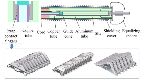
Figure 1.
Schematic diagram of the electrical connection structure used in high voltage bushings.
2.1. Mathematical Model of ECR in Rough Surface
Since the geometric size of the strap contacts is much smaller than the overall conductive structure of the bushing, the concept of total ECR is generally used to describe the electrical connection state of the bushing conductive structure. The body resistance “Rb1” of the strap contact itself and the sum of its “RC1” and “RC2” are regarded as the total ECR “Rt,” and the bulk resistances Rb2 and Rb3 of the central guide rod and the conductor terminal are added to obtain the total resistance Rm of the electrical connection structure, as shown in Figure 2. The morphology of the contact area at the top of the contact observed via laser confocal microscopy is shown on the left side of the figure.
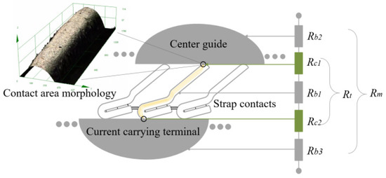
Figure 2.
Schematic diagram of the microscopic morphology and electrical contact resistance of the strap contacts.
It can be seen from the figure that the central rod is in contact with the top of the strap contacts, and the conductor terminal is in contact with both sides at the bottom. Since the radius of curvature of the guide rod is much larger than that of the contour of the strap contacts, the contact surface of the guide rod can be approximated as a semi-infinite plane at the macroscopic level, and the contact surface of the strap contact is approximated as a cylindrical surface. When the central rod is eccentric, once the plane moves down, the gap becomes smaller, and the pressure of the guide rod to the strap contacts increases accordingly, enhancing the fit between the contact surfaces and vice versa.
At the microscopic level, the increase of pressure will lead to an increase in the contact area, and the number of rough peaks under the pressure of the central rod will increase accordingly. When the roughness is constant, the rough peaks meet the Gaussian distribution law [26]. The heights of the asperities are not identical, and not all asperities in the contact area are in contact. Therefore, the analysis of the relationship between the ECR and pressure needs to start from a single rough peak.
The establishment of the classical G-W model is based on the following assumptions:
- (1)
- The surface of the asperities is spherical with the same radius of curvature.
- (2)
- The distribution of the asperities is isotropic, and the heights of all asperities are distributed arbitrarily.
- (3)
- In the process of surface contact, the morphology of the macroscopic matrix does not change. Only the rough peaks are deformed after being compressed. The contact rough peaks do not affect each other.
In the G-W model, the contact between two rough surfaces is equivalent to the contact between a smooth rigid plane and a rough surface [26]. The ECR G-W model of the strap contact described in this section regards the contact surface of the central rod as a smooth rigid plane and the contact surface of the strap contact as a rough cylindrical surface, as shown in Figure 3.
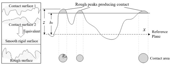
Figure 3.
Schematic diagram of the rough peaks of a random surface conforming to a Gaussian distribution.
Based on the above assumptions, the ECR model of a single roughness peak is first established. The height of the rough peak is set to zero as a baseline, the distance between the reference line and the rigid plane is h0, the distance from the peak to the reference line is the peak height z, and the top of the rough peak can be regarded as a hemisphere with a radius of curvature R. It can be seen that only rough peaks with peak heights greater than h0 can make effective contact. Assuming that the deformation of a single asperity peak under compression is z − h0 > 0, according to the Hertz contact theory [27], only the elastic deformation process of the asperity peak is considered. Then, the actual contact area Ae, pressure Fe, and equivalent modulus on the contact surface of the asperity peak E are expressed as follows:
In the equation, R is the curvature radius of the top of the single roughness peak. E1 and ν1 are the elastic modulus and Poisson’s ratio of the central rod, respectively. E2 and ν2 are the elastic modulus and Poisson’s ratio of the strap contact, respectively. Since the parameter of the curvature radius of the top of the single roughness peak is deduced in the following derivation, there is no need to determine the value, and the surface roughness of the contact is provided by the MC Company [28]. The values of the parameters required for the calculation are shown in Table 1.

Table 1.
Numerical calculation parameters of ECR of strap contacts.
According to R. Holm’s contact model [4], the contact radius a and contact area ECR Rc after a single rough peak is compressed are as follows:
In Equation (5), ρ1 and ρ2 represent the resistivities of the material in the contact area between the central rod and the contact. The values are shown in Table 1.
The contact length of a single asperity peak is the diameter of the asperity peak. If the contact length of the contact under different pressures is obtained, the calculation of the ECR of a single asperity peak can be completed.
where ρ is the equivalent resistivity on the contact surface and L is the contact length of a single asperity peak.
Since only rough peaks with a height greater than h0 can achieve true full contact and bear all the pressure applied by the central rod to strap contacts, the model considers that the contact is a collection of rough peaks conforming to a Gaussian distribution, that is, the actual contact of the surface with the smooth rigid surface is the random contact of multiple rough peaks with the rigid surface. The surface is categorized as a machined surface, and it can be considered that the height distribution of the rough peaks conforms to a Gaussian distribution. According to statistics [29], φ(z) can be used to describe the probability density of the height distribution of multiple roughness peaks on the contact surface. Thus, the probability that the maximum height of the roughness peak is at [z, z + dz] is φ(z)dz. The probability density function φ(z) of the roughness peak height can be expressed as follows:
where σs is the mean square error of the height of the rough surface roughness peaks. The root mean square roughness Rq of the rough surface can be measured with σs. As measured by a laser confocal microscope, the root mean square roughness Rq and arithmetic average roughness Ra of the contact area of the strap contact area satisfy the relationship of Rq = 1.25 Ra.
Assuming that there are a total of N roughness peaks on the macroscopic contact surface with a nominal contact area of An, as mentioned above, only a part of the roughness peaks actually make contact, and the number of roughness peaks in real contact is given by:
The contact lengths of multiple asperity peaks can be obtained by superimposing the diameters of all the asperity peaks in contact. In the range of the effective contact height h from zero to infinity, by integrating all the rough peaks in contact, the total pressure generated by the smooth rigid plane on the rough surface can be obtained. The total contact length and the total pressure are given by:
2.2. ECR Calculation Using G-W Model
A numerical calculation model of the ECR is established according to Equations (10) and (11). The sum of the radius of each roughness peak equals the total contact length. To obtain the relationship between the pressure exerted by the guide rod on the contact finger and the contact resistance of the strap contact finger, it is necessary to create an equation to link the total contact length and the pressure. The ratio of the total contact length of the face to the pressure is as follows:
Since the upper and lower limits of the integral are the same as the integrand variables, the introduction of the dimensionless variables ξ = z/σs simplifies the above equation, and defining the variable ξ0 = h0/σs when z = 0, Equation (12) can be transformed into:
To simplify the complex integral on the right side of Equation (13), the ratio coefficient λ between the total contact length L and the total pressure F on the contact surface is introduced, and the above equation can be simplified as follows:
A curve is fitted to the ratio coefficient of the total contact length to the total pressure of the contact surface λ and the separation variable ξ0, as shown in Figure 4. It can be determined that when the pressure gradually decreases, the distance between the rough peak and the rigid plane becomes larger, resulting in an increase in the separation variable. The ratio of the total contact length with effective contact to the total pressure shows a dynamic increasing trend.
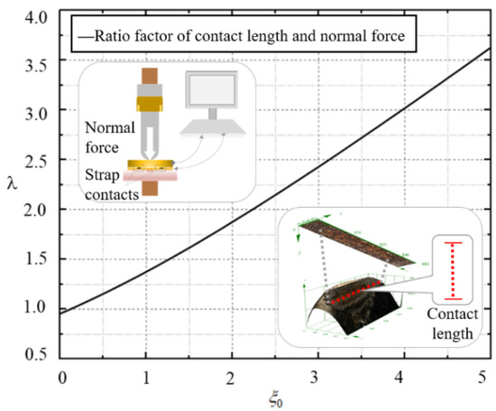
Figure 4.
Relationship between ratio coefficient λ and separation variable ξ0.
When the pressure is constant, the distance between the roughness peak and the rigid plane is constant, and the ratio coefficient is fixed accordingly. It can be seen from Equations (5), (6) and (14) that there is a relationship between the ratio coefficient λ and the ECR; thus, for different contact pressures, this curve can be used as the basis for characterizing the intrinsic relationship between the ECR and the contact pressure F.
According to the relationship between the contact distance and the contact surface roughness in contact mechanics [26], the contact distance between the roughness peak and the rigid plane changes with the surface roughness; thus, the separation variable ξ0 generally fluctuates between 2.5 and 3.5. The roughness of the contact is known, ξ0 is approximately 3.0, and the ratio coefficient can be obtained from the curve to be λ = 2.5. Substituting this into Equation (13), the relationship between contact length and normal force can be approximated as follows:
According to the reciprocal relationship between the conductivity and the resistivity, Equation (5) is converted into Equation (17), and the calculation equation of the ECR after conversion is as follows:
Since the contact surface does not change, the equivalent modulus and the roughness peak height mean square deviation are constants, and the proportionality coefficient is determined using Figure 4. The total contact length can be directly applied under different pressures. Combined with Equation (17), the total ECR and the total pressure exerted of a single-piece strap contact are initially obtained as follows:
The ECR depends on the surface roughness of the contact area, the material parameters, and the pressure [30]. The ECR is inversely proportional to the pressure and is proportional to the equivalent modulus, equivalent resistivity, and mean square error of the surface roughness peak height. The calculation further proves that the eccentricity causes the gap between the central rod and the terminal to be uneven. On the side where the gap becomes smaller, the pressure on the strap contact increases, and the ECR decreases. On the side where the gap becomes larger, the strap touch refers to the reduction of the pressure and the increase of the ECR. Since the contacts of the strap work in series in a loop, the parallel channel is formed when carrying current; thus, an uneven force leads to an overall increase in the ECR. Long-term exposure to a mechanical load leads to the increased surface roughness of the electroplated silver layer on the surface of the contact and the machining, polishing, and grinding of the central rod, the deterioration of the surface material properties, and a proportional increase in the ECR. The two types of influencing factors act together, resulting in an overall increase in the ECR of the bushing electrical connection structure. The content of this section further reflects the important influence of ensuring the coaxiality of the central rod, the smoothness of the surface of the central rod, and the contact for the ECR of the bushing electrical connection structure.
2.3. Correction Factor of G-W Model
A multi-rough peak contact model of the single-piece strap contact was established in previous research according to the classic G-W model. Equation (18) gives the relationship between the ECR of the strap contact and the pressure exerted by the central rod. It is simply considered that the contact surface does not occur. For relative movement, the influence of the force deflection of the contact and the change of the rough peak base profile is not considered. However, in the actual working process, in order to ensure the good contact of the central rod at the contact point of the strap contact, the strap contact is deflected by varying degrees with the change of pressure, as shown in Figure 5, and the contact surface between the contact and the central rod changes [31]. The installation method and the deflection angle of the strap contacts are shown in Figure 6. At the same time, due to the structure of the strap itself, the contact area is a curved surface with different curvature radii, not a plane. In summary, the relationship between the ECR and the pressure should be further revised.
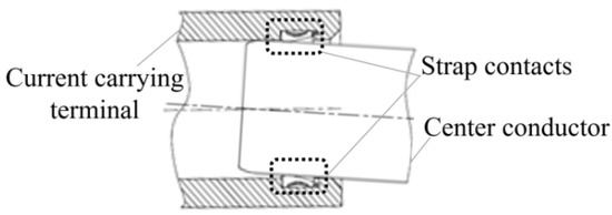
Figure 5.
Changes in the axial contact area of the strap contacts when the copper central rod is eccentric.
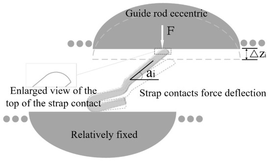
Figure 6.
Schematic diagram of the radial force and deflection of the strap contacts when the copper central rod is eccentric.
When the central rod is eccentric, the upper contact area moves from the top to the left and the lower contact area moves from the top to the right. According to the structure of the contact of the strap, although the contact area changes, the contact surface of the contact is always a cylindrical surface during this process, and no major changes occur.
In addition to the axial deflection, there is also a radial deflection of the strap contacts, as shown in Figure 6. When the central rod has a downward movement, the pressure exerted by the central rod on the top of the strap is F, and the strap deflects radially with the increased pressure. After the downward movement of the central rod is stable, the deflection degree is constant, and the angle between the touch and the horizontal plane changes from ai to ai+1.
To obtain the deflection angle of the strap contact under different pressure conditions, the LA-CUD type strap contact is taken as the research object to study the deflection under different pressures. Since the stainless-steel keel of the touch can be stabilized for a period of time after being pressed, the horizontal angle of the touch is read after waiting for 30 min. Due to the need for correction, the force deflection angle of the contact of the single-piece strap is first sorted out, as shown in Table 2.
Table 2.
Deflection angle of the strap contact fingers under different pressures.
Taking the angle between the contact and the horizontal plane as the benchmark when the single-piece contact is subjected to a central rod pressure of 4 N, the relative deflection angle of the contact shows a trend of first increasing and then decreasing with the increase of pressure. When the pressure is 10 N, the horizontal angle is 19.9°, and the relative deflection angle is 4.7°. According to Table 2, the relationship between the angle ai between the single contact and the horizontal plane and the pressure F is as follows:
It is considered that the effective asperity peak of the contact bears the pressure of the central rod, but practical factors such as the deformation of the base of the asperity peak are not considered. The left side of Figure 2 is an enlarged view of the top profile of the contact of the strap. When the contact is subjected to different pressures, the base of the rough peak changes continuously, that is, the contact point follows the contour line from right to left. To obtain the relationship between the contour and the pressure, the surface profile of the contact is now simplified to a 1/4 circle. The simplified contact profile is shown in Figure 7.
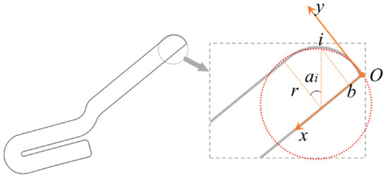
Figure 7.
Schematic diagram of the contour fitting of the contact area.
The contact i under a certain pressure is taken as an example, and point O is taken as the origin to establish a coordinate system. The Ox direction is taken as the x-axis, and the Oy direction is taken as the y-axis. The i point is passed to make a vertical line intersect the x-axis at b, and Ob is recorded as the contact point. The coordinates are determined with the touch point when the pressure is constant. The radius r of the quarter circle is approximately equal to the thickness of a single contact of 0.5 mm, and the relationship between the angle ai of the horizontal plane and the pressure F is fitted with Equation (19). The value of coordinate i is given by:
According to the reciprocal relationship between the conductivity and the resistivity, Equation (5) is converted into Equation (22), and the calculation equation of the ECR after conversion is as follows:
Equations (20) and (21) establish the relationship between the contact point i and the pressure F. The curvature of the top profile of the real strap contacts has a slight variation and is not a complete quarter circle. Therefore, to correct the contour, it is necessary to further establish the relationship between the contour of the real contact and the abscissa of the contact point i. Still taking the coordinate system of Figure 7 as the reference, the ordinate lbi′ is obtained with lob as the dependent variable. The fitting curve obtained by fitting the inverse trigonometric function to the real contour surface of the strap is shown in Figure 8. The fitting equation is as follows:
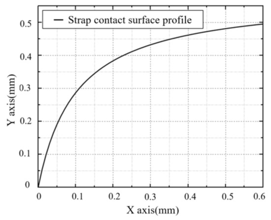
Figure 8.
Contour fitting diagram of the contact area of the strap contact.
Taking the curvature of the surface profile as the independent variable, the relationship between the ECR and the pressure obtained in Equation (18) is corrected, and the correction function a(K) and its parameter K are given by:
In the equation, C1 is related to the equivalent modulus, and C2 and C3 are the correction values of the change trend of the ECR. Combined with Equation (18), the theoretical calculation relationship between ECR and pressure after correction is as follows:
The revised contact resistance calculation model considers the two factors of the deflection and contour, which can further reflect the real working state of the strap contacts and basically achieve the purpose of revision. The calculation process of the revised G-W model is shown in Figure 9.
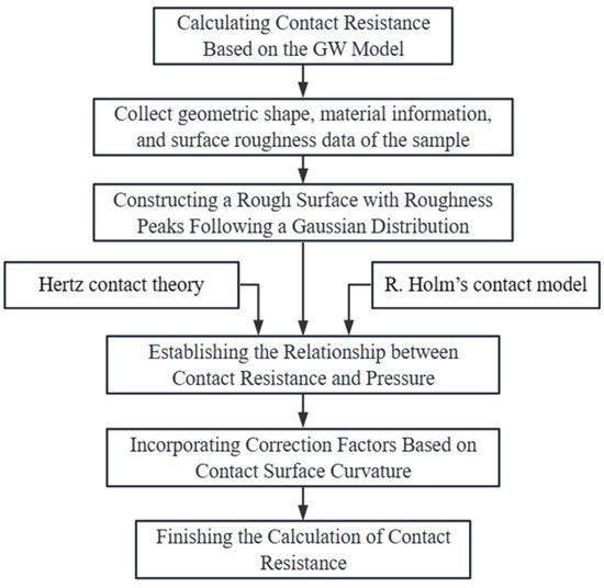
Figure 9.
The calculation process of the revised G-W model.
3. Fractal Model Establishment and ECR Calculation
The rough surface profile of the strap has a complex and fine structure, and it is difficult to describe in classical geometric language. Previous statistical methods based on the G-W model were limited by manual measurements and model simplification, which might have affected the calculated results. However, this shortcoming can be circumvented by the fractal dimension D, which provides a method for describing surface roughness with better accuracy than statistical methods for characterizing and modeling rough surfaces. The fractal dimension D represents the dimension of the graph. The use of fractal geometry to describe and model rough surfaces has strong stability compared to statistical methods, and based on this, Komvopoulos and Ye developed a comprehensive contact analysis that combined the elasticity of contacting rough bodies on rough surfaces. The continuous occurrence of elastic–plastic and fully plastic deformation combined with the fractal topography description can provide guidance for the calculation of the static ECR of strap contacts.
3.1. Area Distribution Function
The M-B fractal contact model [16,32] pointed out that when a fractal rough surface is in contact with an ideal rigid plane, the contact area distribution density function of the asperity is given by:
The real contact area Ar is given by:
where a1 is the contact area of the largest asperity, φ is the fractal area expansion coefficient, and the functional expression [26] for the fractal area expansion coefficient φ and the contour fractal dimension D is as follows:
The surface of the electrical connection structure is machined, and the surface morphology is fine at the atomic scale and still has a fine self-similar structure. The Weierstrass–Mandelbrot fractal function in fractal geometry (W-M function for short) [33] satisfies the self-affineness and other related mathematical properties of rough surfaces; thus, a specific rough surface profile can be represented by a two-dimensional W-M function. The mathematical model of the W-M function is as follows:
where G is the scale parameter of the contour, and D is the fractal dimension of the contour.
The deformation mode of the asperity structure can be divided into three stages: elastic, elastic–plastic, and completely plastic deformation. Figure 10 is a schematic diagram of the contact deformation of a single asperity, where l is the size of the bottom of the asperity, l′ is the cut-off length obtained by using a rigid flat-section asperity, and lr is the asperity when the deformation is ω, the actual contact length. Based on Equation (30), the curvature radius of the top of the asperity can be obtained as follows:
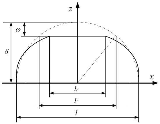
Figure 10.
Schematic diagram of the asperity profile before and after bearing contact pressure.
The height of the asperities is given by:
The actual deformation is given by:
3.2. Elastic Deformation Stage
According to the Hertz theory [27], the maximum contact pressure of asperities is given by:
In the equation, E is the equivalent elastic modulus, which is related to the elastic modulus and Poisson’s ratio of the materials. E can be obtained with Equation (2).
The asperity of the radius R is in contact with a smooth rigid plane, and the critical elastic contact deformation is given by:
where K is the wear coefficient of the material, and is equal to 2.8; and the hardness H and equivalent elastic modulus E conform to the relationship θ = H/E, where H is the hardness of the softer material.
It can also be determined from the Hertz theory that when the asperities are elastically deformed, the actual micro-contact area a is given by:
Substituting Equations (31) and (35) into Equation (36), the critical elastic contact area of the asperities can be obtained as follows:
Combining Equations (31), (34) and (37), it can be determined that when a single asperity is elastically deformed (the critical elastic deformation is also applicable), the relationship between the contact load F and the area a is as follows:
3.3. Elastic–Plastic Deformation Stage
Kogut analyzed the calculation of the contact resistance of a rough surface with different fractal dimensions D and structural parameters G [34] and divided the asperity elastic–plastic deformation into the first and second elastic–plastic deformation zones with 6ωec and 110ωec. The first elastic–plastic deformation zone is ωec < ω < 6ωec, the second elastic–plastic deformation zone is 6ωec < ω < 110ωec, and the critical contact areas formed in these two zones are given by:
3.4. Fully Plastic Deformation Stage
When the actual deformation is greater than 110ωec, the asperities undergo complete plastic deformation, and the relationship between the contact load F and the area a is as follows:
3.5. ECR Calculation for Fractal Conditions
Through the above analysis, it is determined that the contact load and the actual contact area between the rough surface of the finger and the electrode are the sum of the contact load and contact area of all asperities. According to the size and load of the asperities, the deformation of the asperities is divided into elastic deformation, first elastic–plastic deformation, second elastic–plastic deformation, and complete plastic deformation.
Therefore, the actual contact area is the sum of the deformed contact areas described above. When the actual contact area is within the corresponding interval, the actual contact area and the contact load at the time can be uniquely obtained. The actual contact area is calculated as follows:
In the equation, Are is the contact area of elastic deformation, Arep1 is the contact area of the first elastic–plastic deformation, Arep2 is the contact area of the second elastic–plastic deformation, and Arp is the contact area of complete plastic deformation. The true contact load calculation equation is as follows:
It should be noted that since the base length l of the asperities varies with the contact area, that is, for different asperities, the base length l is different, the relationship between the base length l and the contact area is not a known linear relationship. This results in the inability to compute the integral over the base lengths of all asperities.
To solve the above problems, it is assumed that the critical elastic contact area in this research is equal to the critical contact area G2/(Kφ/2)2/(D−1) given by the M-B fractal contact model, which is used to obtain the critical base length lec. In this way, when calculating the contact load of all elastic contact asperities, the base length is regarded as a constant lec, and the critical base length at this time is equivalent to a reference value to describe all asperities, but there are differences between asperities of different sizes. The base length differs from the critical base length by a certain multiple λ; thus, the integral of base length can be equivalent to the integral of λlec. It is found through calculation that the value of λ only affects the magnitude of the load and does not affect the trend of the load change. At this time, the determination of the value of λ only needs to be supplemented by experiments, and the relationship between the actual contact area and the load can be solved:
In Equations (50)–(52), Fre is the contact load of the elastic deformation, Frep1 is the contact load of the first elastic–plastic deformation; Frep2 is the contact load of the second elastic–plastic deformation, and Frp is the contact load of the complete plastic deformation.
The above Equations (50)–(52) are dimensionally normalized, and both sides are divided by E × Aa at the same time. The variables introduced in the dimensioning process are as follows: , , , , and , where is the maximum asperity size. , , , , , and are constants related to the contour fractal dimension. Therefore, for a certain material property θ, fractal dimension D, and scale parameter G, the dimension-one contact load is a function of the dimension-one maximum contact area and the dimension-one true contact area of the asperity.
The relationship between the total contact load Fr* and the real contact area Ar* can be obtained as follows:
In summary, the internal relationship between the actual load P, the contact load Fr, and the actual contact area Ar is derived by combining the fractal theory and empirical equations. Since the applied load P and the contact load Fr are equal, the contact load at each deformation stage of the electrical contact surface of the strap contact can be solved by forming a dimensionless equation with Equation (30), and the theoretical calculation of the contact resistance can finally be realized. Combined with the Holm contact resistance calculation empirical equation, the equation for calculating the contact resistance with the fractal model is derived as follows:
4. Electrical Contact Micromorphology Parameters
4.1. Calculation of Fractal Dimension D
The precise fractal dimension D of the contact points of the strap fingers can be further obtained via combination with the grayscale image method. The acquisition of fractal dimension D is divided into the following three steps:
- (1)
- The three-dimensional structure of the contact area is scanned before and after the test with a laser confocal microscope to obtain real shot, color, and grayscale images.
- (2)
- The grayscale image of 256 × 256 pixels is intercepted, MATLAB is used to identify the image, and the corresponding three-dimensional stereogram is drawn.
- (3)
- The fractal dimension is calculated using the difference box method to obtain D.
The principle of the difference box method is to divide an image of size M × N into several k × k sub-blocks of equal size [21], and the gray value at the image (x, y) is f(x, y), The total gray level is L. At this time, the image is regarded as the surface grayscale set (x, y, f(x, y)) of the three-dimensional object, and the XY plane is a grid of k × k. Each grid has several boxes superimposed, and the height of the box is h = (L − 1) × k/min(M, N). If the mth box contains the grayscale minimum value in the grid in the (i, j) th grid, and the lth box contains the grayscale maximum value in the grid, then the (i, j) th grid is covered. The number of boxes in the lattice is nr (i, j) = l − m + 1. The number of boxes covering the entire grid is Nr = ∑ nr(i, j). From this, the fractal dimension can be calculated as follows:
In the expression, r = k/min(M, N), a set of Nr is calculated by changing the size of the grid k, then the linear regression of the point pair {log(1/r), log(Nr)} is calculated, the slope of which is the fractal dimension D.
Figure 11 shows the fractal dimension D obtained with the contacts in different states. It can be seen that as the magnification increases, the microscopic surface profile does not approach a straight line but rather maintains a roughly similar shape, which proves that the rough surface has geometric self-similarity and the characteristic of self-similarity is scale invariant.
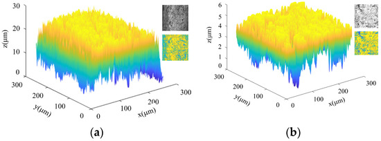
Figure 11.
Contour fitting diagram of the contact area of the strap contact. (a) D = 1.5; (b) D = 1.9.
In this research, the effect of different pressures on the contact resistance under static contact conditions is compared. Therefore, the same contacts under the same conditions are selected for scanning, and the fractal dimension D is obtained from the grayscale images of multiple positions in the contacts. After taking the average value, the fractal dimension D = 1.5 of the contact area in the research object is obtained.
4.2. Calculation of Nominal Contact Area, Aa
According to the above calculation process, when the contact surface parameters remain unchanged, the contact load directly determines the deformation area where the contact is located and the size of the contact area, and there is a one-to-one correspondence between the two. Therefore, the measurement of the micro-morphological parameters of the contact area of the strap’s contact finger is designed and carried out, which provides parameters for the theoretical calculation of the contact resistance of the strap contact’s electrical connection structure.
The test object is the LA-CUD type strap contact. During the test, both sides of the strap contact fingers are adhered inside the L-shaped groove of the tested copper lower electrode to prevent them from coming out. With a certain load, the top contact was in good contact with the tested aluminum upper electrode. Figure 12 shows a three-dimensional real shot and height map of the contact area captured by a laser confocal microscope. The silver-white area, the contact area of the real shot in Figure 12a, is measured using the confocal microscope software, and the projected area of the contact area of a single contact is about 1.3 × 10⁻⁷ m2. As can be seen from Figure 12b, the contact points are irregular surfaces before and after contact, and there is a height difference of 22 microns in the entire contact area. It is difficult to obtain an accurate nominal contact area with the existing methods; thus, the projected area is approximated as the nominal contact area Aa.
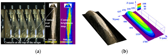
Figure 12.
3D real shot and height map of strap finger contact area as: (a) top view; (b) axonometric view.
5. Measurement of Electrical Contact Resistance
5.1. Test Setup
Two kinds of tests were needed to calculate the ECR for the G-W model, the force deflection verification test of the strap contact and the ECR change test with pressure. The force deflection test measures the deflection of the strap contact with the pressure change. The strap contact was placed between the copper upper electrode and the red copper lower electrode. The specific steps are that the pressure F was applied and the deflection value remained unchanged after 30 min. A laser displacement sensor and an endoscopic microscope were used to record the descending distance of the upper electrode and the deflection posture of the stylus, as shown in Figure 13.
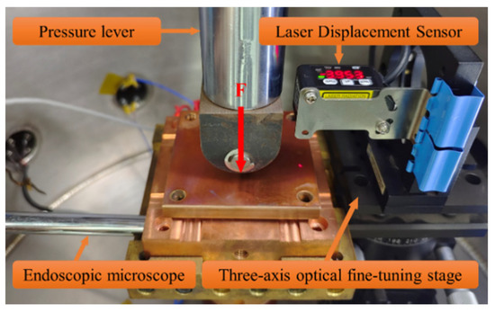
Figure 13.
Verification test device for the force deflection for strap contacts.
During the process of the pressure increase, the dense oxide film formed by the silver-plated layer on the surface of the contact was crushed, the silver layer was squeezed and deformed, obvious deflection marks appeared on the surface of the contact, and the contact surface of the strap changed with the increasing force, as shown in Figure 14. The force deflection process of the contact was corrected. When the pressure of a single contact increased to 10 N, the relative deflection angle was 0.1° and the contact could not continue to deflect. At this time, the contacts overlapped back and forth.
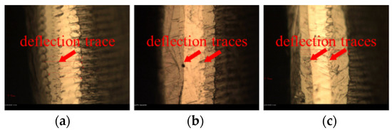
Figure 14.
Deflection marks on straps at different pressures. (a) 4 N; (b) 8 N; and (c) 12 N.
5.2. ECR Measurement
To measure the ECR under different pressures, the current incoming line, the current outgoing line, a millivoltmeter measuring device, and a temperature-measuring thermocouple were added based on the device. In the test, 2 × 12 strap contacts were arranged, and the power supply current was 400 A, which not only met the requirement that the working current of a single contact should be less than 50 A but also reduced the influence of temperature on the contacts.
The test used a current source to supply power. After the power was turned on, the millivolt meter measured the voltage difference between the incoming and outgoing lines of the power supply, as shown in Figure 15. After dividing by the current, the body resistance of the upper and lower plates was subtracted, which was the total resistance of the strap contacts. Each contact was connected in parallel to participate in the current flow; thus, the total resistance was multiplied by the number of sheets to obtain the measured ECR of a single contact. It should be noted that since the ECR of the latter was too small and difficult to measure, the manufacturer did not provide the bulk resistance of the single-piece contact, and the ECR of the strap contact included the body resistance.
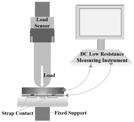
Figure 15.
Contact resistance measurement system.
There are three sources of error introduction in the measurement process. One source was the ECR of the contact surface between the bolt and the electrode, which is unavoidable. The second source was the systematic error of the millivolt meter itself. The third source was the ECR change as the temperature of the contact surface increased and changed. To eliminate the abovementioned errors, first, the same wiring device was used to measure the bulk resistance of the upper and lower electrodes. After subtraction, the measurement error and the systematic error of the millivoltmeter were also subtracted. In the theory of electrical contact, the temperature rise of the contact is difficult to measure experimentally, and the V–T relationship is generally used to calculate the temperature rise of the contact. In 1900, Kohlrausch established the V–T relationship in electrical contacts by using the contact voltage drop as a function of the temperature difference [35]. In the case of electrical-thermal equilibrium and electrical and thermal isolation from the surrounding environment, this relationship is valid for any shape electrical conductivity of similar materials. The contacts were all effective (homogeneous materials refer to materials whose thermal and electrical conductivity quotients are approximate).
Compared with the strap, the base temperature of the contact was increased by 0.22 °C through calculation, the ECR obtained before the subtraction was corrected in combination with the base temperature measured with the thermocouple, and the final ECR measurement value was obtained.
5.3. Experimental and Theoretical Comparisons
The theories of the G-W model and the Fractal model for calculating the contact resistance are analyzed in Section 2, Section 3 and Section 4. Furthermore, the experiment on the strap contact was conducted as described in Section 5.1 and Section 5.2. This section describes how the comparison of the two theoretical models for calculating the contact resistance was conducted.
For the Fractal model, the fractal dimension provides a way to describe the roughness with consideration of the fact that the contact area where the strap comes in contact is very irregular and shaped like a cylindrical surface. This research combines image recognition technology, and a more realistic fractal dimension D was obtained. However, surfaces with completely different structures may also have similar or even the same fractal dimension D, indicating that the fractal dimension D on its own cannot uniquely determine the surface. The structure parameter G can better solve this problem. The larger the structure parameter G is, the greater the selected area is, and the larger the morphology is. The structural parameter G affects the amplitude of the contour and influences the contact resistance of the strap contact finger. According to the structure size and machining parameters of the contact finger of the strap, the G parameter of the strap used in this paper was set as 1 × 10⁻⁷.
Based on the obtainment of the fractal dimension D and the structural parameter G, through the establishment and modification of the statistical model described in Section 2 and the establishment and calculation of the fractal model in Section 3, combined with the selection of the parameters of the fractal calculation in Section 4, the two methods with the G-W model and the fractal model were used to calculate the ECR of the contact under the same load. Moreover, the two theory results are compared with the tested ECR.
It can be seen from Figure 16a that when the load is in the range of 1–10 N, the calculated results of the modified G-W model and the fractal model are generally higher than the experimentally measured values, and the change trends are similar. When the fractal dimension D is 1.5 and the load is 5 N, the calculated ECR of the strap contact finger with the G-W model and the fractal model is 424 μΩ and 418 μΩ, respectively, which are larger than the rated value of 320 μΩ of the ECR of the strap contact made by the MC company, and are closer to the experimental ECR value of 355 μΩ with a 5 N load.
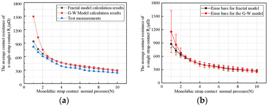
Figure 16.
(a) ECR of the strap contact changing with the pressure; (b) the error bars of the ECR calculated by the fractal model and the G-W model.
After the correction, the G-W model shows a trend of first decreasing sharply and then decreasing slowly. This is because when the load is small, the contact surface of the contact finger is a curved surface, the distance between the two surfaces is large, and the number of rough peaks actually contacted at the edge of the contact surface decreases exponentially; thus, the change of the load has a dramatic effect on ECR. As the load increases, the contact finger deflects and the contour of the base gradually becomes smoother. At this time, the curvature of the contact surface between the contact finger and the guide rod is small; thus, the variation is smaller.
The fractal theoretical model shows that the electrical contact area of the strap contact is in the first elastic–plastic deformation stage, and the contact resistance consists of two stages of elastic and elastic–plastic deformation. When the load of the single contact finger is 1–3 N, the overall contact resistance is high. With the increase of the load, the contact area increases, and the contact resistance decreases slowly.
It can be seen from the error bar in Figure 16b that after the correction, the error of the G-W calculation result is 41%, and the largest relative error of the fractal theory calculation result is 14%. When the load is small (1–3 N), the maximum G-W error is 41%, and the fractal model method has a maximum error of 9%. When the load is normal (4–6 N), the results of the two are almost the same, and the errors are both within 9%. When the load is too large (7–10 N), the results of the two are almost the same, and the errors are within 14%.
In conclusion, the error of the fractal model is smaller and the change trend is closer to the experimental value. In particular, when the contact load is in the middle or low load range, the calculation results of the fractal model are better than the calculation results of the statistical model (G-W model).
To explore the influences of different surface topographies and contact loads on the contact resistance and the actual contact area Ar* of different contact fingers, the electrical connection structure of the contact fingers was determined by changing the fractal dimension D of the contact surface and the load range. The relationship between the actual contact area Ar* of the electrical contact and the load Fr* in the two stages of the elastic deformation and the first elastic–plastic deformation was obtained, as shown in Figure 17.
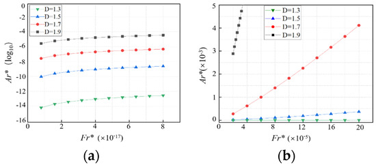
Figure 17.
ECR of the strap contact changing with the pressure at (a) Elastic deformation stage; (b) First elastic–plastic deformation stage.
Figure 17a shows the relationship between Fr* and Ar* when D = 1.3, 1.5, 1.7, and 1.9 in the elastic deformation stage of the rough surface of the finger. It can be seen from the figure that when the load is small, the asperities on the surface of the contact finger only deform elastically, and Fr* is proportional to Ar* during elastic deformation. When the load increases, the asperities on the surface of the contact finger undergo elastic–plastic deformation. At this time, Fr* and Ar* are approximately linearly related.
Since elastic deformation is a recoverable initial stage, small load changes cause large fluctuations in the contact area. The variation trend of the actual contact area with different fractal dimensions is similar; thus, with the increase of D, the actual contact area increases exponentially and the numerical difference is large.
Figure 17b shows the relationship between Fr* and Ar* for different fractal dimensions D in the first elastic–plastic deformation stage of rough surfaces. When the fractal dimension D is the same, it can be seen that the relationship between Fr* and Ar* is approximately linear and the slope changes slightly. With the increase of the fractal dimension D, the straight line slopes of Fr* and Ar* also increase, and the increase range increases. This is because the larger D is, the more complex the microscopic morphology of the rough surface is, and the greater the number of asperities on the surface under the unit area is, the lower the contact pressure and the deformation of the asperities on the rough surface for the same actual contact area are, which increases the bearing capacity of a single asperity.
5.4. Equivalence and Practicality
In the construction of ultra-high voltage (UHV) transmission lines, although the strap contact is a small structure in the high-voltage bushing, it assumes the role of conductive and thermal expansion and the contraction margin. This study combines the traditional ECR calculation with the calculation of the ECR of the contact of a high-voltage bushing strap for the first time.
In engineering practice, the suitable pressure range of the strap contact is 2.5–5 N. When the single chip pressure is 5 N, the rated ECR of the strap provided by the manufacturer is 320 μΩ. Due to measurement error and other reasons, the ECR obtained by the test was 355 μΩ, and the relative error of 11% was acceptable; thus, the test measurement has authenticity and validity.
To date, there has been no systematic research around the world on the operation state of the strap contact structure commonly used in bushing, and the strap contact suppliers cannot provide the operating data of their products under various working conditions. There have been many electrical insulation faults caused by the deterioration of the electrical contacts of strap contacts. Due to the lack of relevant data support, effective solutions and fault diagnosis methods have not been found. Therefore, the theoretical research discussed in this paper compares two methods for theoretically calculating the ECR of the contacts of a strap, which provides theoretical support for revealing the relationship between the change trend of the ECR and the actual operating conditions, and has strong engineering practicability.
6. Conclusions
- (1)
- In this study, the G-W theoretical model and the fractal theoretical model for calculation of the contact resistance of strap contacts used in bushings were investigated. According to the force deflection, the contour correction factor is introduced according to the force of the strap contacts, and the G-W model is further improved.
- (2)
- Using MATLAB and confocal microscopy, the fractal dimension and nominal contact area of the strap contact used in bushing equipment were obtained. Four deformation processes of the strap contacts, elastic, first elastic–plastic, second elastic–plastic, and fully plastic deformation, were added into the fractal theory and the equations were derived.
- (3)
- One strap contact resistance measuring device was designed to carry out the test of contact resistance as a function of the pressure. The actual situation of the force deflection was verified, the thermal resistance increase caused by the contact temperature rise was corrected, and the ECR test value was finally obtained with different loads.
- (4)
- The contact resistances calculated with the two theories were generally higher than the measured data. After the correction, the error of the G-W calculation results was 41%, and the relative error of the fractal theory calculation results was 14% at most. When the load was small (1–3 N), the maximum error of G-W was 41%, and the maximum error of the fractal model method was 9%. As the load increased, the errors of both were within 14%. The error of the fractal model was smaller, and the change trend was closer to the experimental value, which is suitable as a relatively better ECR analytical calculation theory.
- (5)
- It is determined that Fr* and Ar*are proportional in the elastic deformation stage of the strap contact. When the first elastic–plastic deformation occurs, the relationship between Fr* and Ar* is linearly proportional. With the increase of the fractal dimension D, the ECR value of the strap contacts decreases.
Author Contributions
Conceptualization, L.Z.; methodology, J.C.; program writing, T.R.; validation, S.J.; formal analysis, S.J. and Q.W.; data curation, Q.W.; writing—original draft preparation, T.X.; writing—review and editing, X.Z.; supervision, P.L.; project administration, Z.P.; funding acquisition, Q.W. All authors have read and agreed to the published version of the manuscript.
Funding
This research was funded by the National Engineering Research Center of UHV Technology and Novel Electrical Equipment Basis (NELUHV-2021-KF-07).
Data Availability Statement
The data presented in this study are available on request from the corresponding author. The data are not publicly available due to their massive size.
Conflicts of Interest
The authors declare no conflict of interest.
References
- Liu, Z. UHV AC and DC Power Grid; China Electric Power Press: Beijing, China, 2013. [Google Scholar]
- Xie, G.; Shi, S.; Wang, Q.; Liu, P.; Peng, Z. Simulation and experimental analysis of three-dimensional temperature distribution of +/− 400 kV converter transformer valve-side resin impregnated paper bushing under high current. IET Gener. Transm. Distrib. 2022, 16, 2989–3003. [Google Scholar] [CrossRef]
- Tian, H.D.; Liu, P.; Zhou, S.Y.; Wang, Q.; Wu, Z.; Zhang, J.; Peng, Z. Research on the deterioration process of electrical contact structure inside the ±500 kV converter transformer RIP bushings and its prediction strategy. IET Gener. Transm. Distrib. 2019, 13, 2391–2400. [Google Scholar] [CrossRef]
- Holm, R. Electrical Contacts; Springer: New York, NY, USA, 1979. [Google Scholar]
- Greenwood, J.A.; Williamson, J.B.P. Contact of nominally flat surfaces. Proc. R. Soc. A Math. Phys. Eng. Sci. 1966, 295, 300–319. [Google Scholar]
- Greenwood, J.A.; Tripp, J.H. The elastic contact of rough spheres. J. Appl. Mech. 1967, 1, 153–159. [Google Scholar] [CrossRef]
- Bush, A.W.; Gibson, R.D.; Thomas, T.R. The elastic contact of a rough surface. Wear 1975, 35, 87–111. [Google Scholar] [CrossRef]
- Mccool, J.I. Comparison of models for the contact of rough surfaces. Wear 1986, 107, 37–60. [Google Scholar] [CrossRef]
- Greenwood, J.A. A simplified elliptic model of rough surface contact. Wear 2006, 261, 191–200. [Google Scholar] [CrossRef]
- Carbone, G. A slightly corrected Greenwood and Williamson model predicts asymptotic linearity between contact area and load. J. Mech. Phys. Solids 2009, 57, 1093–1102. [Google Scholar] [CrossRef]
- Persson, B.N.J.; Albohr, O.; Tartaglino, U.; Volokitin, A.I.; Tosatti, E. On the nature of surface roughness with application to contact mechanics, sealing, rubber friction and adhesion. J. Phys. Condens. Matter 2004, 17, R1–R62. [Google Scholar] [CrossRef]
- Zhao, Y.W.; Maietta, D.M.; Chang, L. An asperity microcontact model incorporating the transition from elastic deformation to fully plastic flow. J. Tribol. 2000, 122, 86–93. [Google Scholar] [CrossRef]
- Kucharski, S.; Klimczak, T.; Polijaniuk, A.; Kaczmarek, J. Finite elements model for the contact of rough surfaces. Wear 1994, 177, 1–13. [Google Scholar] [CrossRef]
- Kogut, L.; Etsion, I. Elastic-plastic contact analysis of a sphere and a rigid flat. J. Appl. Mech. 2002, 69, 657–662. [Google Scholar] [CrossRef]
- Zhao, Y.; Lu, Y.; Jiang, J. A new rough surface elastic-plastic contact model. J. Mech. Eng. 2007, 43, 95–101. [Google Scholar] [CrossRef]
- Majumdar, A.; Bhushan, B. Fractal model of elastic-plastic contact between rough surfaces. ASME J. Tribol. 1991, 113, 1–11. [Google Scholar] [CrossRef]
- Berry, M.V.; Lewis, Z.V.; Nye, J.F. On the Weierstrass-Mandelbrot Fractal Function. Proc. R. Soc. 1980, 370, 459–484. [Google Scholar]
- Grossmann, S.; Löbl, H.; Böhme, H. Contact Lifetime of Connections in Electrical Power Systems. In Proceedings of the 16th International Conference on Electrical Contacts, Loughborough, UK, 7–11 September 1992. [Google Scholar]
- Song, S.; Wang, L.; Xue, E. Fractal theory and its application in mechanical joint surface. Machinery 2008, 10, 1–3, 7. [Google Scholar]
- Jiang, Z.; Wang, H.; Fei, B. Research into the application of fractal geometry in characterizing machined surfaces. Int. J. Mach. Tools Manuf. 2001, 41, 2179–2185. [Google Scholar] [CrossRef]
- Kennechj, F. Fractal Geometry-Mathematical Foundations and Applications; John Wiley & Sons: London, UK, 1990. [Google Scholar]
- Majumdar, A.; Bhushan, B. Role of Fractal Geometry in Roughness Characterization and Contact Mechanics of Surfaces. Trans Asme J. Tribol. 1990, 112, 205–216. [Google Scholar] [CrossRef]
- Yang, H.; Fu, W.; Wang, W. Calculation model of the normal contact stiffness of joints based on the fractal geometry and contact theory. J. Mech. Eng. 2013, 49, 102–107. [Google Scholar] [CrossRef]
- Morag, Y.; Etsion, I. Resolving the contradiction of asperities plastic to elastic mode transition in current contact models of fractal roughsurfaces. Wear 2007, 262, 624–629. [Google Scholar] [CrossRef]
- Liou, J.L.; Chi, M.T.; Lin, J.F. A microcontact model developed for sphere- and cylinder-based fractal bodies in contact with a rigid flat surface. Wear 2010, 268, 431–442. [Google Scholar] [CrossRef]
- Zhang, L.; Xiao, H.; Dong, H. Statistical research on rough surfaces. Surf. Technol. 2011, 40, 96–100. [Google Scholar]
- Hertz, H. On the elastic contact of elastic bodies. J. Reine. Angew. Math. 1881, 92, 71–156. [Google Scholar]
- Tian, H. Study on Electrical Contact Characteristics and Thermal Effect of Electrical Connection Structure of HVDC Bushings. Ph.D. Thesis, Xi’an Jiaotong University, Shaanxi, China, 2021. [Google Scholar]
- Chang, W.R.; Etsion, I.; Bogy, D.B. An Elastic-Plastic Model for the Contact of Rough Surfaces. Asme J. Trib. 1987, 109, 257–263. [Google Scholar] [CrossRef]
- Jin, S.; Tian, H.; Wang, H.; Cui, B.; QI, Y.; Liu, P.; Peng, Z. Research on the selection and wear characteristics of UHV GIL electrical contact structure. Power Grid Technol. 2022, 46, 4482–4490. [Google Scholar]
- Liang, X. Research on Mechanical and Electrical Contact Characteristics of Spring Contact Structure; Xi′an University of Technology: Xi′an, China, 2020. [Google Scholar]
- Gangepain, J.J.; Roques-Carmes, C. Fractal approach to two dimensional and three dimensional surface roughness. Wear 1986, 109, 119–126. [Google Scholar]
- Komvopoulos, K.; Ye, N. Three-Dimensional contact analysis of elastic-plastic layered media with fractal surface topographies. J. Tribol. 2001, 123, 632–640. [Google Scholar] [CrossRef]
- Kogut, L.; Komvopoulos, K. Electrical contact resistance theory for conductive rough surfaces. J. Appl. Phys. 2003, 94, 3153–3162. [Google Scholar] [CrossRef]
- Konchits, V.V.; Kim, C.K. Electric current passage and interface heating. Wear 1999, 232, 31–40. [Google Scholar] [CrossRef]


Disclaimer/Publisher’s Note: The statements, opinions and data contained in all publications are solely those of the individual author(s) and contributor(s) and not of MDPI and/or the editor(s). MDPI and/or the editor(s) disclaim responsibility for any injury to people or property resulting from any ideas, methods, instructions or products referred to in the content. |
© 2023 by the authors. Licensee MDPI, Basel, Switzerland. This article is an open access article distributed under the terms and conditions of the Creative Commons Attribution (CC BY) license (https://creativecommons.org/licenses/by/4.0/).