Abstract
In view of the application limits of the modified eddy dissipation model (MEDM) in simulations of weakly turbulent flow, compressible flow, and internal flow, an improved eddy dissipation model (IEDM) is proposed. The IEDM model uses the dissociation reactions to obtain the correct combustion temperature instead of the specific heat compensation used in the MEDM model. This extends the application in compressible flow simulation. The simulation accuracy of the IEDM model for weakly turbulent flow is improved by using the accurate transport property and model. The maximum ε/k is limited to give a reasonable reaction rate near walls, and the expression for the model parameter A is also updated. Nine turbulent flames including seven jet flames and two opposed jet flames are simulated with the improved model. Compared with the experimental data of the jet flames, the peak temperature differences with the MEDM model and the IEDM model are 189 and 161 K, respectively, indicating the minor accuracy improvement of the IEDM model. Compared with the experimental data of the opposed flames, the peak temperature differences with the MEDM model and the IEDM model are 131 and 7 K, respectively, indicating the significant accuracy improvement of the IEDM model.
1. Introduction
Because of its simplicity, reasonable accuracy and good convergence, the eddy dissipation model (EDM) is used extensively in turbulent combustion modelling. The model is based on three assumptions: (1) the combustion reaction rate is infinitely fast; (2) the fuel reaction rate in turbulent non-premixed flames only depends on the turbulent mixing rate of the fuel and oxidizer; (3) the fuel reaction rate is inversely proportional to the turbulent time scale, i.e., turbulent kinetic energy divided by turbulent dissipation rate. Based on these assumptions, the following fuel reaction rate expression is given by Magnussen and Hjertager [1].
where f is fuel; o is oxidizer; p is product; S is the stoichiometric mass ratio of oxidizer to fuel; ρ is density; ε is turbulent dissipation rate; k is turbulent kinetic energy; Y is mass fraction; A = 4 is for diffusion flames; and B = 0.5 is for premixed flames. Rf is the fuel reaction rate, which is the sink term in the fuel species transport equation [1]. The product of S and Rf provides the sink term in the oxidizer species transport equation, while the product of (1 + S) and Rf provides the source term in the product species transport equation. The product of heating value and Rf gives the source term in the energy transport equation.
Based on the EDM model, Magnussen [2] developed the eddy dissipation concept (EDC) model later. He further refined and advanced the EDC model in subsequent works [3,4,5]. The EDC model considers the effect of finite reaction rate, which can be used to predict NOx and soot productions. The EDC and EDM models have been implemented in major commercial CFD software, which are used extensively in numerous CFD applications. Unlike the EDC model, which needs to solve numerous stiff elementary reaction rates, the EDM model is fast and very simple, with reasonable accuracy and good convergence.
The EDM model has been investigated for its applicability to scramjet design by simulating three hydrogen-fueled scramjet configurations. The study highlights the importance of case-specific calibration, which can yield reasonably accurate predictions while reducing computational costs [6,7]. In Gobbatto et al. [8], the EDM model is used in the numerical simulation of a hydrogen-fueled gas turbine combustor. Due to the uncorrected A value in the EDM model, a discrepancy arises in the axial coordinate of the temperature peaks. However, when non-dimensional values are considered, a close agreement is observed between the CFD profiles and experimental data at the combustor discharge. The numerical simulations using the EDM model accurately predict the flow field, temperature, mixture fraction, species concentration and heat flux distribution in an industrial boiler [9]. These predictions are validated by comparing them with the available experimental data, demonstrating their reliability and accuracy. The EDM model is used for the numerical simulations of diesel combustion [10]. The results indicate that the EDM model accurately captures the observed trend in pressure rate in both the SANDIA combustion vessel and the Fiat engine.
Wang [11] simulated 11 turbulent non-premixed flames including 7 round jet flames and 4 opposed jet flames with the EDM model and compared the simulation result with the experimental data. It is found that the temperature simulation accuracy is not good with A = 4. For the opposed jet flames, the simulated flame temperature deviates from the experimental data as much as 481 K. The optimal A values are found to match the axial experimental peak temperature. However, the optimal A values vary with the individual flames and correlate with the turbulent Reynolds number in the reaction zone of the flames (the higher the Reynolds number, the smaller the A value). Inspired from the correlation of the optimal A value with the turbulent Reynolds number, Wang [11] proposed and validated the modified eddy dissipation model for diffusion flames.
where Ret,local is the local turbulent Reynolds number; μ is the dynamic viscosity; l is the turbulence integral length; and CD = Cμ3/4 = 0.093/4 = 0.164 is the turbulence constant [12]. Unlike the EDM model with constant A, the MEDM model uses variable A in the combustion region, and the variable A value is determined by a local turbulent Reynolds number. The average of the axial peak temperature difference between the simulation and experiment of the seven jet flames is reduced from 153 to 73 K. The average of the axial peak temperature difference between the simulation and experiment of the opposed jet flames is reduced from 451 to 80 K. The simulation accuracy is greatly improved with the MEDM model.
The EDM model has problems for the simulation of weakly turbulent flows and compressible flows. The MEDM model inherits these disadvantages. In this paper, the defects of the MEDM model are analyzed, and the corresponding corrections are implemented to form the IEDM model. There are three major improvements for the IEDM model: (1) the IEDM model uses the dissociation reactions to obtain the correct combustion temperature instead of the specific heat compensation used in the MEDM model; (2) the accurate transport property and model are used to improve the simulation accuracy for weakly turbulent combustion; (3) the maximum ε/k is limited to give a reasonable reaction rate near walls, the minimum Ret,local is limited for the prediction of weakly turbulent combustion, and the expression for Alocal is updated. The accuracy of the IEDM model is then verified with the experimental data of seven jet flames and two opposed jet flames.
2. IEDM Model
For the EDM and MEDM models, the one-step irreversible reaction is used for the combustion with excessive oxygen: CnHm + (n + m/4)O2 = nCO2 + (m/2)H2O. Since dissociation of combustion products such as H2O and CO2 is not considered, the predicted temperature will be higher than the actual temperature. There are two methods to correct this problem. The first one is the specific heat compensation method, which is used in the MEDM model. The enthalpy–temperature polynomial functions (the NASA 14 coefficient polynomial functions) of O2, H2O, N2, and CO2 have been modified to reflect the temperature drop by dissociation (only for the temperature range of more than 1000 K; the dissociation is negligible if the temperature is less than 1000 K). For a given constant pressure, e.g., 1 atm, an equilibrium composition and temperature calculation (constant pressure and enthalpy condition) for 3000 K H2O is set up, and the calculated equilibrium temperature with dissociation is 2578.4 K; this way, the enthalpy and temperature after dissociation are obtained. Through polynomial function fitting with enough data points, the new polynomial coefficients (a1~a6) of the NASA format are obtained. Using the new specific heat for O2, H2O, N2, and CO2 in the simulation will predict the real combustion temperature. The second method is to include the elementary dissociation reactions in the simulation:
2H + M = H2 + M, H + OH + M = H2O + M, H + O + M = OH + M, CO + O(+M) = CO2(+M)
The specific heat compensation method only modifies the specific heat, and it needs no extra computation effort. This method is recommended for the combustion simulations with constant pressure. The specific heat, the specific heat ratio, and the average molecular weight are critical for compressible flow simulations. The specific heat compensation method does not give accurate values for these parameters. The dissociation reaction method simulates the dissociation process with the elementary reactions, which increases the computation effort significantly. However, it predicts accurate gas composition, specific heat, and the specific heat ratio. It is suitable for compressible flow simulations. For incompressible flows, the simulation accuracy of the two methods is the same. Figure 1 shows the axial temperature distribution of the atmospheric turbulent H2 round jet flame (jet nozzle diameter 3.75 mm, jet velocity 296 m/s, and coflow air velocity 1 m/s [13,14]) with the two methods (the EDM model is used for the combustion modelling), and their results are consistent (the transport model difference is also shown in the figure, which will be explained later). The red dotted curve (specific heat, constant transport) of Figure 1 comes from Wang [11], and the details of the simulation setup can be found there.
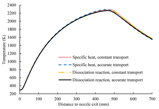
Figure 1.
Comparison of axial temperature profiles with different dissociation compensation methods and transport properties.
For compressible flows, especially supersonic flows, the two methods will have obvious differences in their simulation results. A simple hydrogen/oxygen rocket engine combustion chamber is constructed to illustrate this problem. As shown in Figure 2, the Star-CCM+ software is used to simulate the axisymmetric rocket engine with a combustion chamber length of 1000 mm, chamber radius of 40 mm, and throat radius of 5 mm. The inlet gas temperature is 300 K. The mass flow rates of H2 and O2 are 0.1125 and 0.9 g/s, respectively. The K-Omega SST model is used for turbulence modeling, and the MEDM model is used for combustion modeling. Case A uses the specific heat compensation method, while case B uses the dissociation reactions. The dissociation reaction rates are from the UCSD mechanism [15], which is extensively used and validated [16,17,18,19,20,21]. The geometry and boundary setup are shown in Figure 2.
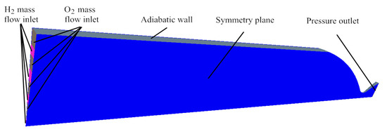
Figure 2.
Geometry and boundary setup of rocket engine simulation.
Figure 3 shows the simulated temperature contours. The temperatures in the chamber of the two cases are almost the same. The mass-flow averaged temperature at plane 1 of case A is 3433.9 K, while that of case B is 3431.2 K, and the difference is only 3 K. However, the temperature contours show significant differences in the region near the throat, where the compressible effect is strong. The mass-flow averaged temperature at the pressure outlet of case A is 2840.9 K, while that of case B is 1997.4 K. The absolute pressures of the two cases are almost constant in plane 1, and those of case A and case B are 0.8178 and 0.8509 MPa, respectively. The pressure difference is 0.0331 MPa, and the relative difference is 3.9%. Figure 4 shows the variation in the specific heat and molecular weight with a radius in plane 1. The average specific heat (0.5 × minimum value + 0.5 × maximum value) of case A is 14167.6 J/Kg/K, which is much higher than the normal average value 3287 J/Kg/K of case B. The average specific heat ratio of case A is 1.0359, which is much smaller than 1.2087 of case B. Moreover, the average molecular weight of case A is 17.21 g/mol, which is larger than that of case B 15 g/mol.
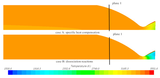
Figure 3.
Temperature contours of the simulation result (only part of the chamber is shown).
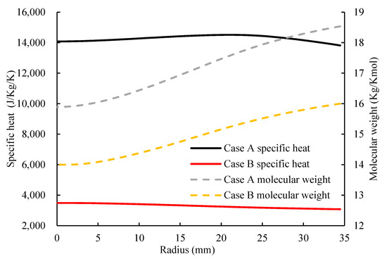
Figure 4.
Specific heat and molecular weight of case A and case B.
The transport properties such as dynamic viscosity (1.81 × 10⁻⁵ pa·s), thermal conductivity (0.0264 W/m/K), and mass diffusivity (3.0 × 10⁻⁵ m2/s) are set to constants in the MEDM model. This is fine for simulations of strongly turbulent flows since turbulent mixing is much stronger than laminar mixing. Using accurate transport properties and models increases the computation effort, and it has almost no effect on the result. Figure 1 shows the axial temperature comparison of the jet flame with different transport calculation methods. One method uses constant viscosity, conductivity and mass diffusivity. Another method uses accurate transport models: the mixture property calculation with mixture averaged rules, the viscosity and conductivity calculation with the polynomial functions of temperature for each species, and the mass diffusivity and mass diffusion calculation with the kinetic theory. The results of the two methods are consistent since the flow is a strongly turbulent flow. However, for weakly turbulent flows, the turbulent mixing rate is on the order of the laminar mixing rate. Accurate calculation of laminar mixing is very important. Using constant transport properties will greatly underestimate the momentum, species and energy diffusion effects. Since the viscosity is no longer a constant with the accurate transport model, the A expression should be updated because the value of Ret,local is different now.
For the simulations near walls, the turbulent kinetic energy k is very small, and the dissipation rate ε is very large, which leads to a very high ε/k value and which overestimates the reaction rate. It is reasonable to limit the ε/k value near walls. Zhukov [22] limited the value of ε/k to 10,000 s−1 when simulating the combustion in a satellite thruster. This value is adopted for the IEDM model.
Considering all the above factors, the IEDM model is proposed:
- One-step combustion reaction: CnHm + (n + m/4)O2 = nCO2 + (m/2)H2O;
- Combustion reaction rate:
- 3.
- Elementary reversible dissociation reactions:
2H + M = H2 + M, H + OH + M = H2O + M, H + O + M = OH + M, CO + O(+M) = CO2(+M)
- 4.
- Accurate transport setup, including mixture property calculation with mixture averaged rules, conductivity and viscosity calculation with polynomial functions of temperature for each species, and mass diffusivity and mass diffusion calculations with kinetic theory.
- 5.
- To avoid an excessive A value when Ret,local is too small in a weakly turbulent combustion flow, the minimum Ret,local is limited to 5.3.
3. CFD Setup
Nine flames including seven non-premixed jet flames and two opposed jet flames are simulated to validate the IEDM model. The International Workshop on Measurement and Computation of Turbulent Non-premixed Flames of the Sandia National Lab (http://www.sandia.gov/TNF/ (accessed on 8 March 2023)) provided a lot of experimental data of the jet flames. Seven of them (Table 1) are used here: flame 1 and flame 2 are the H2/HE round jet flames measured by Barlow and Carter [13,14]; flame 3 is the H2/N2 round jet flame measured by Meier et al. [23]; flame 4 and flame 5 are the H2/N2/CO round jet flames measured by Barlow et al. [24] and Flury [25]; and flame 6 and flame 7 are the H2/N2/CH4 round jet flames measured by Bergmann et al. [26], Meier et al. [27], and Schneider et al. [28]. Two CH4/air opposed jet flames (Table 2) were measured by Mastorakos et al. [29,30,31] (flame 8 and flame 9).

Table 1.
Description of round jet flames.
Table 2.
Description of opposed jet flames.
The air coflow exits of the experimental apparatus for the jet flames are squares, and they are very large relative to the fuel nozzles. Thus, their shapes do not influence the flames, and the flames are axisymmetric. In the simulations, the squares are converted to the circles with the same area. This makes the geometry axisymmetric, and only a sector needs to be simulated. The length in the axial direction is more than 1.5 times the flame height (the axial distance from the fuel nozzle exit to the axial peak temperature location); the length in the radial direction is more than the coflow radius. Figure 5 shows the mesh and boundary setup for flame 1. Except for the mesh along the axis that comprises triangular prisms, the mesh comprises hexahedrons. The cell number is 66,878. The mesh is not uniformly distributed, and there is more mesh set in the combustion region and the region with large gradients. Mesh independence was tested by changing the mesh density.
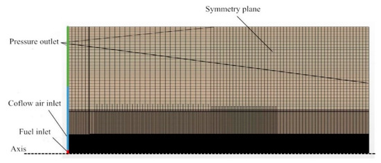
Figure 5.
Mesh and boundary setup for flame 1.
The opposed jet flame 8 is also axisymmetric, so that only a sector is modeled. The mesh and boundary setup are shown in Figure 6. The cell number is 16,100. The mesh next to the axis comprise triangular prisms, and the remaining mesh comprise hexahedrons.
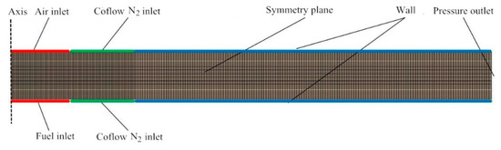
Figure 6.
Mesh and boundary setup for flame 8.
The k-ε/low Reynolds number turbulence model is used here [32]. The model can be considered as a variant of the standard model, and the major improvement is the damping function for the flow near walls or the weak turbulence flow. When applied to round jet flows, this turbulence model generates errors. It overpredicts the spreading rate, which leads to shorter flame length than reality. Following Hossain and Malalasekera [33], Dally et al. [34], Cuoci et al. [35], and The International Workshop on Measurement and Computation of Turbulent Non-premixed Flames of the Sandia National Lab (http://www.sandia.gov/TNF/ (accessed on 8 March 2023)), the correction developed by Morse [36] is used here, modifying the model constant Cε1 (the original value is 1.44) in the turbulent dissipation rate transport equation. An optimal Cε1 with the IEDM model is examined to match the axial peak temperature location between the simulation and the experiment (the optimal Cε1 values with the EDM and the MEDM models are almost the same as those with the IEDM model), and different flames have different optimal Cε1 values as listed in Table 3. The same Cε1 is used for the simulations with the EDM, MEDM and IEDM models of the same flame.
Table 3.
Turbulence model constant Cε1 for different flames.
The turbulence boundary conditions at the inlets are set according to the experimental data. For those flames without these data, the 5% turbulence intensity and the turbulence integral length of 10% inlet diameter are set. The NASA 14 coefficient polynomial functions are used for the specific heat calculation of each species.
The dynamic viscosity and the thermal conductivity of each species are calculated with the format used in CHEMKIN, , , and the coefficients are outputted from CHEMKIN. The mixture properties are calculated with the mass weighted averaging method. The multi-component mass diffusion is calculated with kinetic theory. The gas is set to an incompressible ideal gas (the gas density is calculated with the ideal gas law and the atmospheric pressure, i.e., the density only varies with temperature) since the flow is an open flow. The buoyancy effect is considered. Since the sizes of the flames are very small, their optical thicknesses meet the optical thin criteria. The thermal radiation loss of the combustion product (CO, H2O, and CO2) is calculated as a heat sink in the enthalpy equation.
T∞ is the ambient temperature; σ is the Stefan–Boltzmann constant; Kp is the Planck mean absorption coefficient of the gas; Pi and Ki are the partial pressure of the species i and its Planck mean absorption coefficient, respectively. The Planck mean absorption coefficients of CO, H2O, and CO2 are from Ju et al. [37]. The IEDM and MEDM models are implemented through field functions. The chemical kinetics (dissociation reaction) are accurately and efficiently calculated with the CVODE solver in Star-CCM+.
The conservation equations of the CFD setup are the Favre-averaged partial differential equations for density, three velocity components, species mass fractions, enthalpy, turbulent kinetic energy, and turbulent dissipation rate. The turbulent combustion model (Equations (6)–(8)) provides the source terms in the species transport equations and the enthalpy conservation equation. The thermal radiation heat loss provides a sink term in the enthalpy conservation equation. The segregated solver is used to solve the partial differential equations. The Hybrid Gauss–LSQ (least square method) scheme is used for the numerical solution of the secondary gradients of the diffusion terms and the pressure gradient. The second-order upwind scheme is used for the numerical solution of the convection terms.
4. Results and Discussion
Figure 7 shows the temperature contour simulated with the IEDM model of flame 1 (only part of the geometry is shown for all the contour figures). Table 4 shows the axial peak temperature of the jet flames simulated with the three models, and the difference between the numerical and experimental values are also listed. For the EDM model, it always overpredicts the axial peak temperature. Most of the temperature differences are between 100 and 200 K. The temperature difference of flame 4 is the largest one (283 K), and the temperature difference of flame 2 is the smallest (98 K). The overall accuracy with the MEDM model is obviously better. The temperature difference shows the positive and negative values, and most of the temperature differences are within 100 K. The temperature difference of flame 4 is the largest (189 K). The accuracy of the IEDM model is slightly improved compared with that of the MEDM model. Most of the temperature differences are within 90 K, and the error of flame 4 is the largest (161 K).
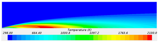
Figure 7.
Simulated temperature contour with IEDM of jet flame 1.
Table 4.
Experimental and numerical axial peak temperatures of jet flames.
The axial temperature profiles are compared in Figure 8 for flame 1. The simulation results with the EDC model are also shown for comparison. The temperature profile with the EDM model is similar to that of the EDC model. The radial temperature profiles are compared in Figure 9 and Figure 10 for flame 1 (the fuel nozzle exit is at Z = 0 mm). The axial temperature profiles are compared for flame 3 and flame 6 in Figure 11 and Figure 12, respectively. The temperature profiles with the IEDM and MEDM models are similar, and they are in good agreement with the experimental results. Since the jet flames are incompressible external flow with strong turbulence, it is natural that the IEDM model has the same prediction accuracy as the MEDM model.
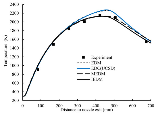
Figure 8.
Axial temperature profile comparison of jet flame 1.
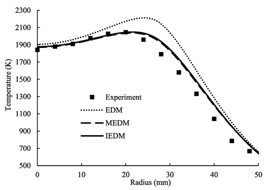
Figure 9.
Radial temperature profile comparison of jet flame 1 (axial height Z = 253.125 mm).
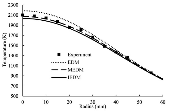
Figure 10.
Radial temperature profile comparison of jet flame 1 (axial height Z = 506.25 mm).
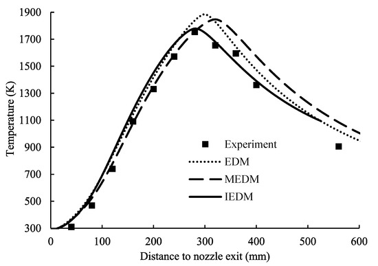
Figure 11.
Axial temperature profile comparison of jet flame 3.
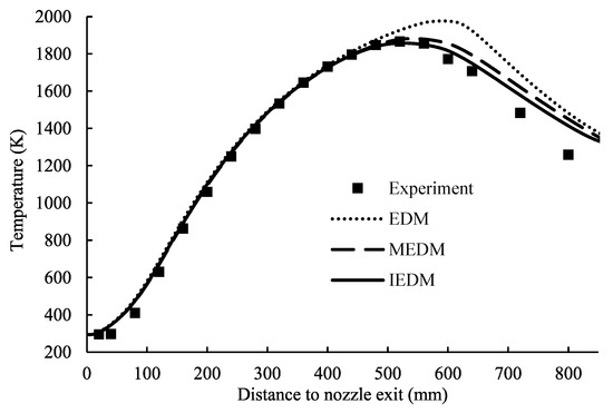
Figure 12.
Axial temperature profile comparison of jet flame 6.
Figure 13 shows the temperature contour simulated with the IEDM model of the opposed jet flame 9. Table 5 shows the axial peak temperature of the opposed jet flames calculated with the three models, and the difference between the numerical and experimental values are also listed. For the EDM model, it always underpredicts the axial temperature. The maximum error is as much as 481 K. These flames are weakly turbulent flows. The local turbulent Reynolds number in the high-temperature zone is on the order of 4–8. By using the accurate transport model, limiting the minimum Ret,local, and updating the A expression, the IEDM model predicts the opposed jet flames accurately. The errors with the IEDM model are in the single digits, as shown in Table 5.
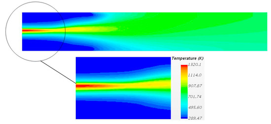
Figure 13.
Simulated temperature contour of the opposed jet flame 9.
Table 5.
Experimental and numerical axial peak temperatures of the opposed jet flames.
The numerical and experimental axial temperature profiles are compared in Figure 14 and Figure 15 for flame 8 and flame 9, respectively. The numerical temperature profiles with the three models are similar. The simulated peak temperature position is slightly toward the fuel nozzle for flame 8. The EDM simulations with the accurate transport model and the dissociation reactions are also shown in Figure 14 for comparison. The peak temperature increases 63.9 K with the accurate transport model, indicating that the transport model can improve the accuracy of the EDM model for the weakly turbulent flow. The dissociation reaction only increases the peak temperature by 17 K. Considering the peak temperature increase of 474 K with the IEDM model, most of the accuracy improvement on the IEDM model results from the combustion reaction rate updating.
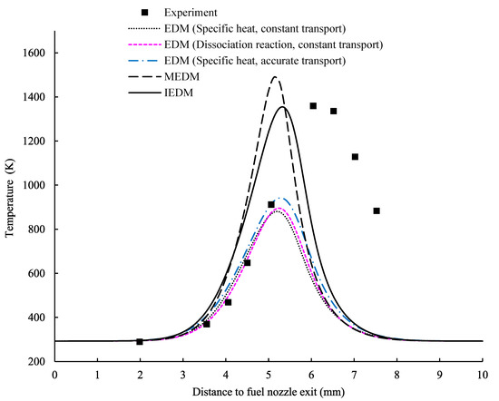
Figure 14.
Axial temperature profile comparison of opposed jet flame 8.
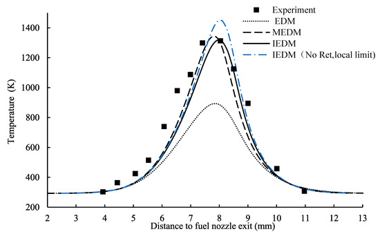
Figure 15.
Axial temperature profile comparison of opposed jet flame 9.
Figure 16 shows the Ret,local contour simulated with the IEDM model. The black line frame in the figure shows the region where Ret,local is less than 5.3. The region is at the position where the axis intersects with the stagnation surface, and the average Ret,local in this region is 4.42. The axial velocity on the stagnation surface is zero, and the radial velocity on the axis is zero; thus, the velocity is very small close to the interaction region. If Ret,local is not restricted, the value of Alocal will be too large. Consequently, Rf is overestimated, leading to a significantly higher peak temperature than the experimental value, as shown in Figure 15 (137 K more than the experimental value).
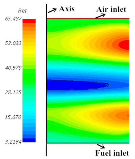
Figure 16.
Simulated Ret,local contour of opposed jet flame 9.
5. Conclusions
Considering the problems in the applications of the MEDM model in compressible flow, weakly turbulent flow, and internal flow, the model is further developed. Three major corrections are implemented: (1) Using the dissociation reactions instead of the specific heat compensation will give a correct value for the specific heat ratio and molecular weight, which will improve the simulation accuracy for compressible flow. (2) Using accurate transport properties and the model will improve the simulation accuracy for the weakly turbulent flow. (3) Limiting the maximum ε/k value will improve the simulation accuracy near walls. Limiting the minimum local turbulent Reynolds number will ensure that the reaction rate is reasonable in a weakly turbulent flow simulation. The A value expression is also updated. Through these corrections, an improved eddy dissipation model is obtained.
The jet flames and the opposed jet flames are simulated with the IEDM model, and the results are compared with the experimental data. For the jet flames, the temperature profiles with the IEDM and MEDM models are similar, and both models outperform the EDM model in the flame temperature prediction accuracy. Compared with the experimental data, the maximum axial peak temperature differences of the EDM, MEDM and IEDM models are 283, 189, and 161 K, respectively. Compared with the experimental data of the opposed jet flames, the maximum axial peak temperature differences of the EDM and MEDM models are 481 and 131 K, respectively. By using the accurate transport model, limiting the minimum Ret,local, and updating the A value expression, the maximum axial peak temperature differences of the IEDM model are in the single digits. Without limiting Ret,local, the simulated axial peak temperature of flame 9 will be 137 K more than the experimental value.
In summary, for strongly turbulent flows and incompressible flows, the temperature simulation accuracy with the IEDM model is slightly better than those with the MEDM model. For weakly turbulent flows and compressible flows, the IEDM model demonstrates obvious advantages.
Author Contributions
Validation, X.L.; Data curation, X.L. and Y.C.; Writing—original draft, X.L. and Y.C.; Writing—review & editing, P.W. All authors have read and agreed to the published version of the manuscript.
Funding
This research received no external funding.
Data Availability Statement
Data available on request from the authors.
Conflicts of Interest
The authors declare no conflict of interest.
References
- Magnussen, B.F.; Hjertager, B.H. On mathematical modeling of turbulent combustion with special emphasis on soot formation and combustion. Symp. Combust. 1977, 16, 719–729. [Google Scholar] [CrossRef]
- Magnussen, B.F. On the Structure of Turbulence and a Generalized Eddy Dissipation Concept for Chemical Reaction in Turbulent Flow. In Proceedings of the 19th Aerospace Sciences Meeting, St. Louis, MO, USA, 12–15 January 1981; Volume 42. [Google Scholar] [CrossRef]
- Magnussen, B.F. Modeling of NOx and soot formation by the eddy dissipation concept. In Proceedings of the International Flame Research Foundation First Topic Oriented Technical Meeting, Amsterdam, The Netherlands, 17–19 October 1989. [Google Scholar]
- Magnussen, B.F. The eddy dissipation concept: A bridge between science and technology. In Proceedings of the ECCOMAS Thematic Conference On Computational Combustion, Libson, Portugal, 21–24 June 2005; Volume 21. [Google Scholar]
- Gran, I.R.; Magnussen, B.F. A numerical study of a bluff-body stabilized diffusion flame. Part 1. Influence of turbulence modeling and boundary conditions. Combust. Sci. Technol. 1996, 119, 171–190. [Google Scholar] [CrossRef]
- Hoste, O.E.J.J.; Fossati, M.; Taylor, J.I.; Gollan, J.R. Modeling scramjet supersonic combustion via eddy dissipation model. In Proceedings of the 68th International Astronautical Congress (IAC), Adelaide, Australia, 25–29 September 2017. [Google Scholar]
- Hoste, O.E.J.J. Scramjet Combustion Modeling Using Eddy Dissipation Model. Ph.D. Thesis, University of Strathclyde Department of Mechanical and Aerospace Engineering, Glasgow, Scotland, 2018. [Google Scholar]
- Gobbato, P.; Masi, M.; Toffolo, A.; Lazzaretto, A. Numerical simulation of a hydrogen fuelled gas turbine combustor. Int. J. Hydrogen Energy 2011, 36, 7993–8002. [Google Scholar] [CrossRef]
- Carvalho, M.d.G.; Coelho, P.J. Numerical prediction of an oil-fired water tube boiler. Eng. Comput. 2009, 3, 227–234. [Google Scholar] [CrossRef]
- D’Errico, G.; Ettorre, D.; Lucchini, T. Comparison of Combustion and Pollutant Emission Models for DI Diesel Engines. SAE Pap. 2007, 45, 2007–2024. [Google Scholar] [CrossRef]
- Wang, P. The model constant A of the eddy dissipation model. Prog. Comput. Fluid Dyn. Int. J. 2016, 16, 118. [Google Scholar] [CrossRef]
- Tannehill, J.; Anderson, D.; Pletcher, R. Computational Fluid Mechanics and Heat Transfer, 2nd ed.; Taylor & Francis: Abingdon, UK, 1997. [Google Scholar]
- Barlow, R.; Carter, C. Raman/Rayleigh/LIF measurements of nitric oxide formation in turbulent hydrogen jet flames. Combust. Flame 1994, 97, 261–280. [Google Scholar] [CrossRef]
- Barlow, R.; Carter, C. Relationships among nitric oxide, temperature, and mixture fraction in hydrogen jet flames. Combust. Flame 1996, 104, 288–299. [Google Scholar] [CrossRef]
- Chemical-Kinetic Mechanisms for Combustion Applications, San Diego Mechanism Web Page, Mechanical and Aerospace Engineering (Combustion Research), University of California at San Diego, 15 August 2016. Available online: http://web.eng.ucsd.edu/mae/groups/combustion/mechanism.html (accessed on 8 March 2023).
- Bramlette, R.B.; Depcik, C.D. Review of propane-air chemical kinetic mechanisms for a unique jet propulsion application. J. Energy Inst. 2020, 93, 857–877. [Google Scholar] [CrossRef]
- López-Cámara, C.F.; Saggese, C.; Pitz, W.J.; Shao, X.; Im, H.G.; Dunn-Rankin, D. Reduced chemical kinetic model for CH4-air non-premixed flames including excited and charged species. Combust. Flame 2023, 253, 112822. [Google Scholar] [CrossRef]
- Drost, S.; Aznar, M.S.; Schießl, R.; Ebert, M.; Chen, J.-Y.; Maas, U. Reduced reaction mechanism for natural gas combustion in novel power cycles. Combust. Flame 2021, 223, 486–494. [Google Scholar] [CrossRef]
- Laksana, A.; Patki, P.; John, T.; Acharya, V.; Lieuwen, T. Distributed heat release effects on entropy generation by premixed, laminar flames. Int. J. Spray Combust. Dyn. 2023; online first. [Google Scholar] [CrossRef]
- Xiang, L.; Jiang, H.; Ren, F.; Chu, H.; Wang, P. Numerical study of the physical and chemical effects of hydrogen addition on laminar premixed combustion characteristics of methane and ethane. Int. J. Hydrogen Energy 2020, 45, 20501–20514. [Google Scholar] [CrossRef]
- Siatkowski, S.; Wacko, K.; Kindracki, J. Extensive study on the detonation cell size of biogas-oxygen mixtures. Fuel 2023, 344, 128016. [Google Scholar] [CrossRef]
- Zhukov, V.P. Computational fluid dynamics simulations of a GO2/GH2 single element combustor. J. Propuls. Power 2015, 6, 1707–1714. [Google Scholar] [CrossRef]
- Meier, W.; Prucker, S.; Cao, M.-H.; Stricker, W. Characterization of Turbulent hytVAir Jet Diffusion Flames by Single-Pulse Spontaneous Raman Scattering. Combust. Sci. Technol. 1996, 118, 293–312. [Google Scholar] [CrossRef]
- Barlow, R.S.; Fiechtner, G.J.; Carter, C.D.; Chen, J.Y. Experiments on the scalar structure of turbulent CO/H2/N2 jet flames. Combust. Flame 2000, 120, 549–569. [Google Scholar] [CrossRef]
- Flury, M. Experimentelle Analyse der Mischungstruktur in Turbulenten Nicht Vorgemischten Flammen. Ph.D. Thesis, ETH, Zurich, Switzerland, 1998. [Google Scholar]
- Bergmann, V.; Meier, W.; Stricker, D.W. Application of spontaneous Raman and Rayleigh scattering and 2D LIF for the characterization of a turbulent CH4/H2/N2 jet diffusion flame. Appl. Phys. B 1998, 66, 489–502. [Google Scholar] [CrossRef]
- Meier, W.; Barlow, R.S.; Chen, Y.L.; Chen, J.Y. Raman/Rayleigh/LIF measurements in a turbulent CH4/H2/N2 jet diffusion flame: Experimental techniques and turbulence–chemistry interaction. Combust. Flame 2000, 123, 326–343. [Google Scholar] [CrossRef]
- Schneider, C.; Dreizler, A.; Janicka, J.; Hassel, E. Flow field measurements of stable and locally extinguishing hydrocarbon-fuelled jet flames. Combust. Flame 2003, 135, 185–190. [Google Scholar] [CrossRef]
- Mastorakos, E. Turbulent Combustion in Opposed Jet Flows. Ph.D. Thesis, Imperial College London, University of London, London, UK, 1993. [Google Scholar]
- Mastorakos, E.; Taylor, A.M.; Whitelaw, J. Extinction and temperature characteristics of turbulent counterflow diffusion flames with partial premixing. Combust. Flame 1992, 91, 40–54. [Google Scholar] [CrossRef]
- Mastorakos, E.; Taylor, A.M.K.P.; Whitelaw, J.H. Scalar dissipation rate at the extinction of turbulent counterflow nonpremixed flames. Combust. Flame 1992, 91, 55–64. [Google Scholar] [CrossRef]
- Lien, F.S. Low-Reynolds-Number Eddy-Viscosity Modelling Based on Non-Linear Stress-Strain/Vorticity Relations. In Proceedings of the 3rd Symposium on Engineering Turbulence Modelling and Measurement, Heraklion, Greece, 27–29 May 1996; Volume 3, pp. 91–100. [Google Scholar]
- Hossain, M.; Malalasekera, W. Modelling of a bluff body stabilized CH4/H2 flame based on a laminar flamelet model with emphasis on NO prediction. Proc. Inst. Mech. Eng. Part A J. Power Energy 2003, 217, 201–210. [Google Scholar] [CrossRef]
- Dally, B.B.; Fletcher, D.F.; Masri, A.R. Flow and mixing fields of turbulent bluff-body jets and flames. Combust. Theory Model. 1998, 2, 193–219. [Google Scholar] [CrossRef]
- Cuoci, A.; Frassoldati, A.; Ferraris, G.B.; Faravelli, T.; Ranzi, E. The ignition, combustion and flame structure of carbon monoxide/hydrogen mixtures. Note 2: Fluid dynamics and kinetic aspects of syngas combustion. Int. J. Hydrogen Energy 2007, 32, 3486–3500. [Google Scholar] [CrossRef]
- Morse, A.P. Axisymmetric Turbulent Shear Flows with and without Swirl. Ph.D. Thesis, London University, London, UK, 1977. [Google Scholar]
- Ju, Y.; Guo, H.; Liu, F.; Maruta, K. Effects of the Lewis number and radiative heat loss on the bifurcation and extinction of CH4/O2-N2-He flames. J. Fluid Mech. 1999, 379, 165–190. [Google Scholar] [CrossRef]


Disclaimer/Publisher’s Note: The statements, opinions and data contained in all publications are solely those of the individual author(s) and contributor(s) and not of MDPI and/or the editor(s). MDPI and/or the editor(s) disclaim responsibility for any injury to people or property resulting from any ideas, methods, instructions or products referred to in the content. |
© 2023 by the authors. Licensee MDPI, Basel, Switzerland. This article is an open access article distributed under the terms and conditions of the Creative Commons Attribution (CC BY) license (https://creativecommons.org/licenses/by/4.0/).