Abstract
In the thermal industry, one common way to transfer heat between hot tubes and cooling fluid is using cross-flow heat exchangers. For heat exchangers, microscale coatings are conventional safeguards for tubes from corrosion and dust accumulation. This study presents the hypothesis that incorporating domain knowledge based on governing equations can be beneficial for developing machine learning models for CFD results, given the available data. Additionally, this work proposes a novel approach for combining variables in heat exchangers and building machine learning models to forecast heat transfer in heat exchangers for turbulent flow. To develop these models, a dataset consisting of nearly 1000 cases was generated by varying different variables. The simulation results obtained from our study confirm that the proposed method would improve the coefficient of determination (R-squared) for trained models in unseen datasets. For the unseen data, the R-squared values for random forest, K-Nearest Neighbors, and support vector regression were determined to be 0.9810, 0.9037, and 0.9754, respectively. These results indicate the effectiveness and utility of our proposed model in predicting heat transfer in various types of heat exchangers.
1. Introduction
Coatings are applied to improve various properties, such as corrosion resistance, abrasion resistance, toughness, chemical resistance, etc. Some of the most common materials used for coating purposes are polyurethane foams because of their simple handling, economic cost, and proper physical properties [1,2,3]. In the most recent decade, researchers have studied how coating thickness affects heat transfer in finned-tube heat exchangers [4,5]. An accurate estimation of coating thickness is crucial to increase heat exchanger lifetime, especially in high working temperatures [6]. Machine learning methods have recently attracted much attention alongside the usual approaches to heat transfer and thermodynamics analysis. For instance, estimating the heat values of different kinds of fuel with machine learning methods is faster and computationally cheaper than direct calculations and experiments [7,8]. Machine learning models are also employed to predict optimal system design. Mohamed et al. suggested multiple machine learning models to predict eleven different parameters for proton exchange membrane (PEM) electrolyzer cells to achieve optimum design [9]. Recently, machine learning has shown great promise in computational fluid dynamics (CFD) studies [10] and is becoming more accurate and faster [11,12]. Making machine learning models with acceptable generalization capabilities for different heat transfer problems is another approach that has made analysis faster. For instance, a universal model for predicting heat transfer that occurs with condensation and pressure drops using machine learning techniques has been recently proposed [13]. These techniques are also used to analyze heat exchangers for different purposes, like predicting the thermal performance of fins for a novel heat exchanger [14]. Lindqvist et al., with machine learning models, successfully optimized heat exchanger designs and developed good correlations with trends in the CFD model [15]. Moreover, machine learning has shown great potential in predicting heat transfer for high-order nonlinear cases [16]. In the absence of a valid physical-based model, machine learning can be utilized to predict heat transfer in many thermal systems [17]. Considering recent advances in machine learning techniques, CFD computational costs can be reduced by using genetic algorithms [18]. Similarly, neural networks have demonstrated their effectiveness in analyzing the thermal conductivity of oil-based nanofluids [19]. Gradient-boosting decision trees can reduce the cost of measuring equipment for computing transient heat flux [20]. Although more advanced ensemble models can lead to better results for more complicated datasets [21], the use of such models for heat transfer problems has received less attention. The most common model of this category, random forest, has shown a remarkable ability to evaluate heat transfer across various scenarios [16]. Swarts et al. compared three different algorithms for predicting the critical heat flux of pillar-modified surfaces and concluded that random forest provides the best results [22]. Its performance with large datasets [23] and a precise ranking of features’ importance [24] are its main benefits. Despite the benefits of random forest and other machine learning algorithms, collecting training data can be a challenge. The number of data required for training can be minimized by combining features, which enhances regression accuracy [25]. Another solution is state-of-the-art machine learning models; to address this, Yuqing Zhou et al. proposed entropy-based sparsity measures for the prognosis of defects, which can evaluate physical degradation phenomena based on impulsive signals and sparsity criteria. That study also introduced a new directed divergence measure and a sparsogram method based on the proposed entropy measure to identify defect-related information in complicated hydraulic machinery, which can be suppressed by deterministic vibration. The sparsogram tool helps to select the appropriate filtering band for envelope analysis [26]. As far as we know, there are no studies on machine learning models that investigate the correlation between coating and heat transfer in a heat exchanger. This study has filled this gap with machine learning models with acceptable generalization capabilities for unseen data, using a new method.
In this study, a new method for combining input features is proposed to investigate the effect of variable coating thickness on the prediction of heat transfer in a finned-tube heat exchanger at different inlet Reynolds numbers. Almost 1000 different cases were simulated using a 3D finite volume model to generate the dataset. The random forest model was initially trained using numerical simulation data. Using the created model, selected features were combined and new features were added. In addition, various new data were used to validate models’ interpolations. Lastly, the capability of the introduced method for dimension reduction was investigated with different models. The main contributions of this study are summed up as follows:
- To the best of our knowledge, this is the first general machine learning model for predicting heat transfer in heat exchangers based on coating thickness over a wide range of domains.
- This paper presents the hypothesis that incorporating domain knowledge based on governing equations can be beneficial for developing machine learning models for CFD results, given the available data. Additionally, this work proposes a novel approach for combining features that have equal impacts on heat transfer, such as coating thickness, resulting in a reduction in the total number of features without compromising the sensitivity of the original feature space.
- The proposed method cures the curse of dimensionality of the K-Nearest Neighbors algorithm, and, as a result, the model accuracy has been significantly improved.
- The feature engineering and feature combination methods used in this work make it possible to train machine learning models for smaller datasets with acceptable accuracy for unseen data from new domains.
Section 2 explores the impacts of the input features on heat transfer and examines the features’ extraction and data collection processes. The proposed method, input features, training strategy, and results are described in Section 3. In Section 4, the results are explained to validate the presented approach with a comparative analysis of different machine learning models. Finally, the last subsection concludes this article.
2. Heat Transfer Analysis and Feature Extraction
The case study in this work was the passage of hot gas flow over a bunch of tubes with a triangular arrangement. An isometric view of the domain is shown in Figure 1a and the geometry dimensions (in mm) are shown in Figure 1b. The symmetry boundary condition was set around the selected volume, shown with dashed lines in Figure 1a. The coating material on each tube was polyurethane, and the coating thickness on each tube was different but in the range of 10–30 µm. The wall temperature of all tubes was assumed to be constant. The gas entered the domain with different Reynolds numbers and temperatures, which caused heat transfer. A finite volume model (FVM) was developed to simulate turbulent gas flow. Table 1 reveals some results from this FVM.

Figure 1.
Computational domain of the gas flow over the tube bundle with a triangular arrangement from the perspective (a) and front views (b). The dimensions are in mm. (Note: tube bundles are numbered sequentially).

Table 1.
Numerical results of different case studies without coatings (cases 1 to 3) and with coating (case 4). t is the average of five tubes’ coating thickness in micrometers. The inlet gas had variable velocities (Vin) in SI units, temperature (Tin) is the inlet temperature in degrees Kelvin, and () is the temperature difference between the tubes and the inlet gas. The last column represents the total heat transfer from the tube walls into the fluid flow.
Figure 2 displays the temperature distribution for the third case’s conditions as presented in Table 1. The purpose of this figure is to provide a visual representation of the relation between temperature and the target variable being studied. The chosen distribution shows the overall trend in the data and was selected for the case with the maximum temperature difference. Due to space constraints, including all temperature groups may not have been necessary if the overall trend were consistent across different temperature groups. In order to understand how coating thickness and Reynolds numbers influence heat transfer, different simulations were performed with variations in coating thickness, Reynolds number and temperature. Figure 3a,b represent the total heat flux and heat transfer coefficients for the last tube in the fluid flow direction. Our simulation results also showed that the change in flow velocity with increasing coating thickness was negligible. Specifically, we found that the velocity change between a case without coating and the maximum coating thickness considered in this paper (30 μm) was less than 0.000029 percent. Therefore, we concluded that it was valid to neglect the impact of coating thickness on flow velocity in this study. Also of note is that the results obtained from the last tube were representative of the impacts of the coating thickness and Reynolds number on the outlet flow. It is worth noting that this was the overall behavior of the heat exchanger and the total heat flux and heat transfer coefficient increases for larger Reynolds numbers, and they both decreased when the coating thickness was increased.

Figure 2.
Temperature (K) profile for conditions of case 2 as presented in Table 1.
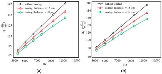
Figure 3.
The total heat flux (normalized by pipes’ total surface area) versus Re number (a) and the heat transfer coefficient of the last tube (#5) versus Re number (b).
2.1. Collected Datasets
These numerical simulations were the basis of forming the dataset. The dataset structure was made in two steps. First, each tube coating thickness was varied within three values, i.e., 10, 20, and 30 μm. Thus, the total number of data (for five tubes) gathered from the simulations was = 243. This dataset was collected by varying the coating thickness values within the three values mentioned before and calculating each case’s total heat transferred from the heat exchanger. In our first analysis, mentioned in Section 3.1, we utilized five features that were fixed and had limited numbers of values (each containing only the three values mentioned above) to calculate the feature importance. Besides the coating thickness, other variables that were not involved in the training process of the first random forest were kept constant throughout its entire training phase. For the next step, after the feature combination process (which is explained in Section 3.2), new variables were added and varied in a wide range of domains; as a result, the final dataset was formed randomly, with 1000 data within range. We analyzed a range of data that included values for T_inlet, T_pipe, velocity, and coating thickness. The maximum values for these variables were found to be 498 K, 298 K, 20 m/s, and 30 μm, respectively. Conversely, the minimum values for these variables were 398 K, 100 K, 6 m/s, and 0 μm, respectively. We also calculated the maximum temperature difference, which was found to be 398 K. To ensure that the context of our analysis remains consistent, more details are provided in Section 3.2.
2.2. Simulation Details and Validation
The present study has investigated the impact of varying coating thickness on the total heat transfer of a system of five aluminum pipes coated with polyurethane. The geometry of the heat exchanger was discretized into control volumes with depths of 5 mm each, and the symmetry condition was applied around the separated volume. The inner wall temperature of all pipes was assumed to be constant and equal, while air entered the system with variable inlet velocity and temperature. Heat transfer occurred between the air and the pipes due to the temperature difference. A finite volume model (FVM) was employed to collect the training data and to evaluate the impact of varying the coating thickness on the total heat transfer. In order to calculate the individual effects of the selected features on the total heat transfer, each feature was varied while the other features were held constant. In this study, to validate the simulations, a comparison of their results with those obtained from the simulations in reference [27] was performed. The only difference between the simulations in this study and those in the reference study is that the former considered the addition of coating to the pipes while the latter incorporated the use of fins. To assess the accuracy of the present study’s results, the temperature distribution calculations obtained were compared with those in reference [27], as depicted in Figure 4. Furthermore, the total outlet temperature and exchanged heat flux per unit of the exchanger surface for different boundaries were compared between this study and reference [27], as presented in Table 2. These comparisons confirm the accuracy and reliability of the results obtained in this study and support their agreement with the findings of reference [27].

Figure 4.
Temperature field comparison with reference [27] in degrees Kelvin.
Table 2.
Comparison of this study and the reference [27] results. Note that units are in m/s, degrees Kelvin and .
Ref. [27]’s model of k-ω turbulence was used to model the heat transfer analysis. To evaluate the accuracy and reliability of our heat transfer model, we performed a sensitivity analysis by varying the input parameters and assessing the resulting changes in the output results. Based on our sensitivity analysis and comparison with the analytical results in Ref. [27], we believe that our heat transfer model provides accurate and reliable results for the problem under investigation, as shown in Table 2. To investigate the effects of mesh refinement on the simulation results, we performed additional simulations using a mesh with higher numbers of nodes and elements. Specifically, we compared the results obtained from the optimal mesh, with 320,787 nodes and 278,136 elements, to those obtained from a mesh with 1,122,814 nodes and 1,055,700 elements. To further improve the accuracy of our results in the second case, we used a higher mesh resolution near the boundaries. Our findings indicated that the difference in the results between the two meshes was negligible, with only a 0.000724% variation observed for a case with an inlet temperature of 498 degrees Kelvin, a pipe temperature of 200 degrees Kelvin, an inlet velocity of 10 m/s, and a coating thickness of 10 μm for all five pipes. Therefore, we conclude that the optimal mesh we used in our initial simulation was sufficient to obtain accurate results for the problem under investigation.
3. Proposed Method
In this study, a random forest algorithm was first trained with a limited dataset to quantify each pipe coating thickness’s impact on the total heat transfer. Our proposed approach enhanced the model’s performance by using domain knowledge to combine related features. To evaluate the capability of this approach, it was validated on a larger dataset with more features. As illustrated in Figure 5, new models were built based on this approach, which reduced the required amount of training data while maintaining the same level of accuracy. This approach demonstrates the potential to optimize machine learning models and improve their efficiency in analyzing complex datasets. Finally, new regression predictors, containing random forest, K-Nearest Neighbors, and support vector regression, were trained using fourfold cross-validation. The hyperparameters of each model were optimized using a random grid approach to identify the best set of hyperparameters to test our approach’s accuracy.

Figure 5.
Flowchart of preparing the machine learning model based on combining important features. Note: the purple dotted box in this figure separates the preprocessing and feature combination methods from the main process.
After the creation of the models, unseen data were used to validate each model generalization. To investigate the models’ accuracy, an R-squared criterion was used as follows: . Note that the best value for this metric equals 1, but it also can be negative if the model were to perform worse than the mean of the data in predicting the observed value.
3.1. Training Model
Random forest quantitatively evaluates each input feature’s importance, but factors like untuned hyperparameters and the total number of observed data can cause a negative impact on the value of each feature’s rank. The number of categories for each input should also be equal for accurate ranking [28]. Tuning hyperparameters is the next step toward having an accurate model. A model’s prediction is more accurate and its ability to rank features’ importance is more precise when its hyperparameters are tuned. Bayesian optimization is used for this [29]. A probability model was built using Bayesian optimization based on past evaluation results; this model estimated the objective function and its uncertainty, and then, with the help of the model, the next set of hyperparameters was selected to estimate the cost function. This process continued with a search-based method to find the best set of hyperparameters. Table 3 shows the selected hyperparameters for this approach. The designed random forest based on the above steps could closely predict the total heat flux for new input features for calculated results, as shown in Figure 6. The random forest regressor fit q near to the FVM results, with R2 = 0.9832 for the training phase and R2 = 0.9864 for the testing phase. The greater value of R-squared in the test dataset indicated that the model was able to perform better on the test dataset than on the training dataset; this is a desirable outcome that indicates that the model has a good generalization capability. One may note that this phase was just a designed pre-task for the model to rank feature importance and that this was not the final model to predict the total heat flux for new input, so there was no need to evaluate this model with unseen datasets. This model calculated the feature importance of the coating thickness variable by measuring how much that variable contributed to the accuracy of predictions. This was automatically carried out with the Scikit-learn library by measuring the reduction in the mean squared error (MSE) of the model when a given predictor variable was used to split the data in a tree. The results are shown in Figure 7. This figure presents how to reduce the size of feature space dimensionality for the main model. Note that in this context, feature space dimensionality refers to the total number of features used to represent the manifold dataset.
Table 3.
Optimization results with Bayesian approach before feature combination.
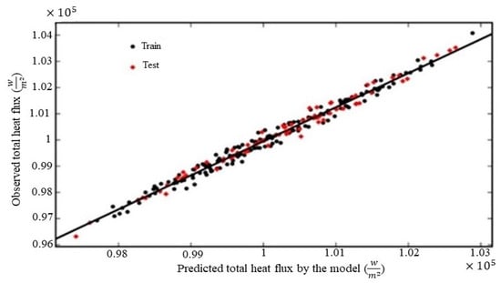
Figure 6.
Comparison of predicted total heat flux (q) with FVM simulations and ML regressor.

Figure 7.
Predictor importance estimation by model.
3.2. Feature Combination and Expanding Model Domain
In order to have a generalized model that could predict the total heat flux (q), new features were added to the feature matrix. Increasing the number of features required more data collection, since data are collected through either numerical simulation or experiments that have costs. A new approach was employed to decrease the total number of required simulations in this work. To do so, a new variable () was defined, as shown in Equation (1):
Based on the results presented in Figure 7, the first five features were combined into one feature; then, three new features were added to the feature matrix. The final feature matrix consisted of four features: inlet velocity; pipe temperature (T_pipe); fluid temperature (T_fluid); and a new variable, , which was introduced to represent the combined effect of the five coating thickness features in the new feature matrix. Using the equivalent coating thickness variable, , we were able to calculate the heat flux values of tubes with different coating thicknesses (t1, t2, t3, t4, t5) with an equivalent case that had ť as the coating thickness for all pipes. Once the features were selected, data collection was initiated. A total of 168 sample cases were simulated and used to create training and testing matrices by randomly varying the inlet velocity, Tpipe, Tfluid, and within the mentioned range in Section 2.1. The purpose of this data collection was to provide a representative sample of the system and to ensure that the training and testing matrices were comprehensive enough to capture the variability of the system. By collecting these data, we were able to train our model to accurately predict the total heat flux based on the selected features. Once again, the hyperparameters were tuned with the Bayesian optimization method. Table 4 shows the hyperparameters designed with this optimization scheme. Figure 8 compares the total heat flux predicted by the random forest and the calculated results from the FVM simulations. The random forest regressor fit q nearly to the FVM results, with R-squared = 0.9994 for the training phase and R-squared = 0.9600 for the testing phase.
Table 4.
Optimization results with Bayesian approach after feature combination.

Figure 8.
Comparison of the total heat flux (q) calculated by the FVM and predicted with random forest after features combination.
As shown in the previous subsection, although the training data were limited for the second random forest with the combined features, the model performed well with the test dataset. Still, the model needed to be evaluated with an unseen dataset. A new dataset was collected in order to study the model performance with new domains for this goal. To elaborate, we chose different Reynolds numbers within the range of interest and used the corresponding velocities as input in our model. Nevertheless, it is essential to understand that this model may not be valid if other terms in the Reynolds number, such as the diameter or viscosity, are changed. The dataset we used contained a total of 549 new cases, which were simulated based on eight variables, [Re, Tpipe, Tfluid, t1, t2, t3, t4, t5], as input, where ti is the coating thickness of tube #i. The total heat flux was predicted with the second random forest, with [Re, Tpipe, Tfluid, ] as input features. Note that ť is calculated with Equation (1), with [t1, t2, t3, t4, t5] as variables. The random forest regressor fit q closely to the observed results, with R2 = 0.9810 for the unseen dataset (see Figure 9).
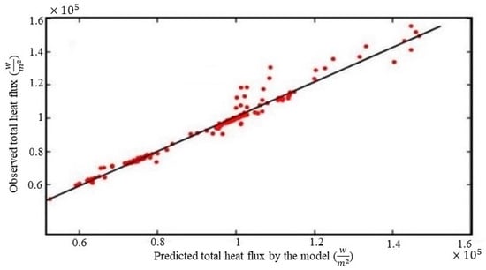
Figure 9.
Validating the model with unseen data.
4. Results and Discussion
In real-world problems in different industries, feature space contains lots of variables that cause training processes to be slow and, in some cases, make it much harder to find good solutions. Theoretically, it is possible to solve these problems by adding new data to training datasets, but collecting new data can be impossible in certain scenarios. Reducing the total number of features is another solution to this problem, but the available approaches may cause some difficulties, like losing information about the original feature space or even making the model perform worse. As indicated in the previous section, combining related features with Equation (1) can save deleted features’ information. Our model can accurately predict heat flux over new, distinct domain features, as shown in Figure 9. The combination process also significantly reduced the amount of data needed to train the model. Alternatively, using a simpler variable, such as the average value of the variables, , instead of , for combining features is not a good choice, since this variable does not take into account any differences between the first and last tube’s heat flux. In addition, the information about the original feature space would be lost (see Table 5).
Table 5.
The total heat flux calculated for different coating thicknesses.
Different models were made to analyze the impact of feature combination. The key to a fair comparison of these models is to make sure that each model is evaluated with the same approach and using the same data. The second random forest training dataset was used to create new models and keep things fair. Each model was trained once with the feature combination technique and once without it. The best combination of hyperparameters was found using a grid search for each model, with a common fourfold cross-validation technique. The results are shown in Table 6.
Table 6.
Comparison of all models (R2).
As shown in Table 6, all models predicted unseen data better after Equation (1) was used to combining features, but the downside is that a primary model is needed to calculate Equation (1)’s coefficients. This may be disadvantageous if obtaining considerably better results is not possible with this method. Conversely, this method can significantly improve the performances of algorithms that are victims of the curse of dimensionality. For example, the K-Nearest Neighbors (K-NN) regressor does not perform well in high-dimension inputs [30], but after feature combination, the K-NN performance increased by 67.66%. Support vector regression (SVR) may also suffer from the curse of dimensionality when enough data samples are not available. This issue can affect the generalization ability of SVR, but after the feature combination, the R-squared value for the unseen data increased by 2.82%. In the case of SVR, one may conclude that increasing the total number of samples may be a better idea than reducing the dimensionality, but as a reminder, we want to mention that SVR does not perform well on large datasets, so increasing the total number of samples may not be a good strategy for this algorithm. Note that the mentioned models were tuned using a grid search approach in which different combinations of hyperparameters were evaluated to minimize the objective function mentioned earlier. The best hyperparameters for models that are made without feature combination are as follows: leaf_size = 64; number of neighbors = 8 for K-Nearest Neighbors; in the case of SVR, rbf kernel is used; and to have more complex boundaries, the value of C, which determines the penalty for misclassifying training data points, is set to a large value, which is 10,000. After use of the feature combination method, new hyperparameters were set for the models. In the case of K-Nearest Neighbors, leaf_size was set to 1 and the total number of neighbors was 4, and for the SVR, once again, rbf kernel was used with the same C value. The last model, random forest, was immune to the curse of dimensionality and overfitting, so there was no need to combine input features, but by comparing the two random forest models in Table 6, one can see that the R-squared value was just slightly improved after the reduction of the total number of inputs. This point shows that after combining features with Equation (1), no information will be lost. To ensure that our high prediction accuracy was not due to fixed features, we compared the standard deviation and the mean of the target between the training and unseen datasets, and we found that [mean, std] = [81,012.245125, 11,028.389484] for training and [mean, std] = [85,333.387071, 19,010.531518] for the unseen dataset, indicating that our model’s performance with the unseen dataset was valid and the model is capable of extrapolating and interpolating, which would have been impossible if the inputs did not have enough diversity. However, it is important to note that our machine learning models were based on the CFD details mentioned earlier, and changing the heat transfer coefficient model could affect this model’s accuracy. Thus, we assume that our model’s best performance on other heat transfer coefficient models would be achieved when those models have similar target values. If this issue were a primary concern, the simplest solution would be to collect data from the considered model and use the type of model as an input feature.
A new feature was also created by combining the Re number and t as input for Equation (1). The trained model with this approach was not as accurate as the previous models. This process raised this question: “When can we use Equation (1)?”. As shown in Figure 7, [t1,t2,t3,t4,t5] have closer importance scores to each other in comparison to the Re number importance score. (Note that the Reynolds number has more impact on heat flux than coating thickness, so its importance score is much higher than s importance score.) By knowing this, it is better to combine features within the same order of magnitude or with similar impacts on the target, like coating thicknesses for different tubes.
5. Conclusions
This work investigated various models of heat transfer correlation to predict total heat flux with varied coating thickness for different conditions. Feature selection was essential before implementation of the machine learning model for studied cases. Despite all the benefits of feature selection, there is a chance of losing important information because of deletion. The employed approach can decrease the size of feature space without losing sensitive knowledge about the main feature space and also showed potential for heat transfer problems in which available data are limited. Training data for the algorithm were obtained with the finite volume model method. The trained model predicted well with the training dataset, with R2 ~ 0.9994, and with the testing dataset, with R2 ~ 0.9600. The algorithm was also able to predict total heat flux, similar to the finite volume model, with R2 ~ 0.9810, based on its interpolation mechanism. Other algorithms, like SVR and K-NN, were also employed to check other aspects of the feature combination method used in this work, and also showed great promise in predicting the total heat transfer based on unseen data, with R2 ~ 0.9754 and R2 ~ 0.9037. For future works, the results of this study may be beneficial for stacking models with better generalization of fewer data.
Author Contributions
Conceptualization, M.J., A.R. and M.A., methodology, M.J., A.R. and M.A.; software, M.J.; collecting data, E.T. and S.A.Z.; review and editing, M.A. and A.R.; funding acquisition, M.A. All authors have read and agreed to the published version of the manuscript.
Funding
This research received no external funding.
Data Availability Statement
Not applicable.
Conflicts of Interest
The authors declare no conflict of interest.
References
- Usman, M.A.; Adeosun, S.O.; Osifeso, G.O. Optimum Calcium Carbonate Filler Concentration for Flexible Polyurethane Foam Composite. J. Miner. Mater. Charact. Eng. 2012, 11, 311–320. [Google Scholar] [CrossRef]
- Lefebvre, J.; Bastin, B.; Le Bras, M.; Duquesne, S.; Paleja, R.; Delobel, R. Thermal stability and fire properties of conventional flexible polyurethane foam formulations. Polym. Degrad. Stab. 2005, 88, 28–34. [Google Scholar] [CrossRef]
- Woods, G. The ICI Polyurethanes Book, 2nd ed.; Allport, D.C., Ed.; John Wiley & Sons: Hoboken, NJ, USA, 1990; p. 1. [Google Scholar]
- Valipour, F.; Dehghan, S.F.; Hajizadeh, R. The effect of nano- and microfillers on thermal properties of Polyurethane foam. Int. J. Environ. Sci. Technol. 2022, 19, 541–552. [Google Scholar] [CrossRef]
- Al-Homoud, M.S. Performance characteristics and practical applications of common building thermal insulation materials. Build. Environ. 2005, 40, 353–366. [Google Scholar] [CrossRef]
- Cheng, Y.; Miao, D.; Kong, L.; Jiang, J.; Guo, Z. Preparation and Performance Test of the Super-Hydrophobic Polyurethane Coating Based on Waste Cooking Oil. Coatings 2019, 9, 12. [Google Scholar] [CrossRef]
- Matveeva, A.; Bychkov, A. How to Train an Artificial Neural Network to Predict Higher Heating Values of Biofuel. Energies 2022, 15, 7083. [Google Scholar] [CrossRef]
- Góra, K.; Smyczyński, P.; Kujawiński, M.; Granosik, G. Machine Learning in Creating Energy Consumption Model for UAV. Energies 2022, 15, 6810. [Google Scholar] [CrossRef]
- Mohamed, A.; Ibrahem, H.; Yang, R.; Kim, K. Optimization of Proton Exchange Membrane Electrolyzer Cell Design Using Machine Learning. Energies 2022, 15, 6657. [Google Scholar] [CrossRef]
- Runchal, A.K.; Rao, M.M. CFD of the Future: Year 2025 and Beyond BT—50 Years of CFD in Engineering Sciences: Commemorative Volume in Memory of D. Brian Spalding; Runchal, A., Ed.; Springer: Singapore, 2020; pp. 779–795. [Google Scholar]
- Alexiou, K.; Pariotis, E.G.; Leligou, H.C.; Zannis, T.C. Towards Data-Driven Models in the Prediction of Ship Performance (Speed—Power) in Actual Seas: A Comparative Study between Modern Approaches. Energies 2022, 15, 6094. [Google Scholar] [CrossRef]
- Andrés-Pérez, E. Data Mining and Machine Learning Techniques for Aerodynamic Databases: Introduction, Methodology and Potential Benefits. Energies 2020, 13, 5807. [Google Scholar] [CrossRef]
- Mosavi, A.; Shamshirband, S.; Salwana, E.; Chau, K.-W.; Tah, J.H.M. Prediction of multi-inputs bubble column reactor using a novel hybrid model of computational fluid dynamics and machine learning. Eng. Appl. Comput. Fluid Mech. 2019, 13, 482–492. [Google Scholar] [CrossRef]
- Krishnayatra, G.; Tokas, S.; Kumar, R. Numerical heat transfer analysis & predicting thermal performance of fins for a novel heat exchanger using machine learning. Case Stud. Therm. Eng. 2020, 21, 100706. [Google Scholar] [CrossRef]
- Lindqvist, K.; Wilson, Z.T.; Næss, E.; Sahinidis, N.V. A Machine Learning Approach to Correlation Development Applied to Fin-Tube Bundle Heat Exchangers. Energies 2018, 11, 3450. [Google Scholar] [CrossRef]
- Kwon, B.; Ejaz, F.; Hwang, L.K. Machine learning for heat transfer correlations. Int. Commun. Heat Mass Transf. 2020, 116, 104694. [Google Scholar] [CrossRef]
- Vu, A.T.; Gulati, S.; Vogel, P.-A.; Grunwald, T.; Bergs, T. Machine learning-based predictive modeling of contact heat transfer. Int. J. Heat Mass Transf. 2021, 174, 121300. [Google Scholar] [CrossRef]
- Nasution, M.K.; Elveny, M.; Syah, R.; Behroyan, I.; Babanezhad, M. Numerical investigation of water forced convection inside a copper metal foam tube: Genetic algorithm (GA) based fuzzy inference system (GAFIS) contribution with CFD modeling. Int. J. Heat Mass Transf. 2022, 182, 122016. [Google Scholar] [CrossRef]
- Jamei, M.; Olumegbon, I.A.; Karbasi, M.; Ahmadianfar, I.; Asadi, A.; Mosharaf-Dehkordi, M. On the Thermal Conductivity Assessment of Oil-Based Hybrid Nanofluids using Extended Kalman Filter integrated with feed-forward neural network. Int. J. Heat Mass Transf. 2021, 172, 121159. [Google Scholar] [CrossRef]
- Wu, W.; Wang, J.; Huang, Y.; Zhao, H.; Wang, X. A novel way to determine transient heat flux based on GBDT machine learning algorithm. Int. J. Heat Mass Transf. 2021, 179, 121746. [Google Scholar] [CrossRef]
- Eskandari, A.; Milimonfared, J.; Aghaei, M. Line-line fault detection and classification for photovoltaic systems using ensemble learning model based on I-V characteristics. Sol. Energy 2020, 211, 354–365. [Google Scholar] [CrossRef]
- Swartz, B.; Wu, L.; Zhou, Q.; Hao, Q. Machine learning predictions of critical heat fluxes for pillar-modified surfaces. Int. J. Heat Mass Transf. 2021, 180, 121744. [Google Scholar] [CrossRef]
- Genuer, R.; Poggi, J.-M.; Tuleau-Malot, C.; Villa-Vialaneix, N. Random Forests for Big Data. Big Data Res. 2017, 9, 28–46. [Google Scholar] [CrossRef]
- Archer, K.J.; Kimes, R.V. Empirical characterization of random forest variable importance measures. Comput. Stat. Data Anal. 2008, 52, 2249–2260. [Google Scholar] [CrossRef]
- Ladha, L.; Deepa, T. Feature Selection Methods and Algorithms. Int. J. Comput. Sci. Eng. 2011, 3, 1787–1797. [Google Scholar]
- Zhou, Y.; Kumar, A.; Parkash, C.; Vashishtha, G.; Tang, H.; Xiang, J. A novel entropy-based sparsity measure for prognosis of bearing defects and development of a sparsogram to select sensitive filtering band of an axial piston pump. Measurement 2022, 203, 111997. [Google Scholar] [CrossRef]
- Bošnjaković, M.; Čikić, A.; Muhič, S.; Stojkov, M. Development of a new type of finned heat exchanger. Teh. Vjesn. Tech. Gaz. 2017, 24, 1785–1796. [Google Scholar] [CrossRef]
- Strobl, C.; Boulesteix, A.-L.; Zeileis, A.; Hothorn, T. Bias in random forest variable importance measures: Illustrations, sources and a solution. BMC Bioinform. 2007, 8, 25. [Google Scholar] [CrossRef]
- Wu, J.; Chen, X.-Y.; Zhang, H.; Xiong, L.-D.; Lei, H.; Deng, S.-H. Hyperparameter Optimization for Machine Learning Models Based on Bayesian Optimizationb. J. Electron. Sci. Technol. 2019, 17, 26–40. [Google Scholar]
- Toth, C.D.; O’Rourke, J.; Goodman, J.E. Nearest neighbours in high-dimensional spaces. In Handbook of Discrete and Computational Geometry, Chapman and Hall; Goodman, J.E., O’Rourke, J., Eds.; CRC: Boca Raton, FL, USA, 2004; pp. 877–892. [Google Scholar]


Disclaimer/Publisher’s Note: The statements, opinions and data contained in all publications are solely those of the individual author(s) and contributor(s) and not of MDPI and/or the editor(s). MDPI and/or the editor(s) disclaim responsibility for any injury to people or property resulting from any ideas, methods, instructions or products referred to in the content. |
© 2023 by the authors. Licensee MDPI, Basel, Switzerland. This article is an open access article distributed under the terms and conditions of the Creative Commons Attribution (CC BY) license (https://creativecommons.org/licenses/by/4.0/).