Article

Accurate Remaining Available Energy Estimation of LiFePO4 Battery in Dynamic Frequency Regulation for EVs with Thermal-Electric-Hysteresis Model

School of Vehicle and Mobility, Tsinghua University, Beijing 100084, China
*
Authors to whom correspondence should be addressed.
Energies 2023, 16(13), 5239; https://doi.org/10.3390/en16135239
Submission received: 23 May 2023 / Revised: 27 June 2023 / Accepted: 30 June 2023 / Published: 7 July 2023
(This article belongs to the Special Issue New Trends in Hybrid Electric Vehicles)

Abstract

:
Renewable energy power generation systems such as photovoltaic and wind power have characteristics of intermittency and volatility, which can cause disturbances to the grid frequency. The battery system of electric vehicles (EVs) is a mobile energy storage system that can participate in bidirectional interaction with the power grid and support the frequency stability of the grid. Lithium iron phosphate (LiFePO4) battery systems, with their advantages of high safety and long cycle life, are widely used in EVs and participate in frequency regulation (FR) services. Accurate assessment of the state of charge (SOC) and remaining available energy (RAE) status in LiFePO4 batteries is crucial in formulating control strategies for battery systems. However, establishing an accurate voltage model for LiFePO4 batteries is challenging due to the hysteresis of open circuit voltage and internal temperature changes, making it difficult to accurately assess their SOC and RAE. To accurately evaluate the SOC and RAE of LiFePO4 batteries in dynamic FR working conditions, a thermal-electric-hysteresis coupled voltage model is built. Based on this model, closed-loop optimal SOC estimation is achieved using the extended Kalman filter algorithm to correct the initial value of SOC calculated by ampere-hour integration. Further, RAE is accurately estimated using a method based on future voltage prediction. The research results demonstrate that the thermal-electric-hysteresis coupling model exhibits high accuracy in simulating terminal voltage under a 48 h dynamic FR working condition, with a root mean square error (RMSE) of only 18.7 mV. The proposed state estimation strategy can accurately assess the state of LiFePO4 batteries in dynamic FR working conditions, with an RMSE of 1.73% for SOC estimation and 2.13% for RAE estimation. This research has the potential to be applied in battery management systems to achieve an accurate assessment of battery state and provide support for the efficient and reliable operation of battery systems.

1. Introduction

1.1. Background

To achieve carbon neutrality, the installed capacity and generation of renewable energy systems such as solar photovoltaic and wind power are continuously increasing [1]. However, these renewable energy systems exhibit intermittency and variability, and the direct integration of their generated electricity into the power grid can cause disturbances to the grid frequency. In a high proportion of renewable energy power systems, to ensure the stability of the power grid frequency, the dispatch center needs to monitor the grid frequency deviation in real-time and issue frequency regulation (FR) instructions to the FR ancillary services market [2]. Lithium iron phosphate (LiFePO4) battery energy storage systems used in electric vehicles (EVs), due to their long cycle life, low cost, and high safety performance, have gradually gained favor from FR service providers, and their market share continues to increase. The participation of energy storage systems in grid FR requires real-time assessment of the battery system’s state of charge (SOC) and remaining available energy (RAE) by the battery management system. Based on the current state of the battery, corresponding control strategies are formulated to prevent overcharging and over-discharging of the battery [3], mitigate safety risks [4], and maximize earnings. Therefore, accurately estimating the battery system’s SOC and remaining energy is crucial. The SOC and RAE of a battery cannot be directly measured; instead, corresponding algorithms need to be designed for estimation. Advanced battery management algorithms are based on battery voltage models [5], and establishing an accurate voltage model is the foundation for state estimation [6]. Under FR working conditions, the current exhibits bidirectional high-frequency pulses, causing a significant rise in internal temperature during the operation of LiFePO4 batteries. The open-circuit voltage (OCV) also exhibits complex hysteresis characteristics, making accurate voltage modeling challenging. Therefore, it is of great research significance for FR working conditions to establish high-precision voltage models that consider multiple influencing factors and to establish accurate state estimation algorithms. These efforts are essential for ensuring precise control, reliable operation, and high efficiency of energy storage systems.

1.2. Literature Review

1.2.1. Lithium-Ion Battery Model

The voltage models for LiFePO4 batteries are divided into electrochemical mechanism models, simplified electrochemical mechanism models, equivalent circuit models (ECMs), and neural network models (NNMs). Doyle et al. [7] used partial differential equations to describe the solid-phase and liquid-phase potential distribution during the charge and discharge process of lithium-ion batteries, as well as the diffusion of lithium ions in the solid phase and the migration of lithium ions in the liquid phase. They proposed the pseudo-two-dimensions (P2D) model. This model achieves high accuracy in terminal voltage simulation but has numerous microscopic parameters, making parameter identification challenging and requiring extensive computational resources. Simplifying the positive and negative electrode active particles as single particles, the single particle (SP) model was proposed [8], which simplifies the computational complexity of the P2D model. The SP model exhibits higher simulation accuracy for the terminal voltage at low current rates, but lower simulation accuracy for the terminal voltage at high current rates. Based on the P2D model, a simplified pseudo-two-dimensions (SP2D) model was proposed by polynomial approximation of the lithium-ion concentration in the electrolyte [9]. The P2D model was linearized to develop the reduced-order model (ROM) for real-world applications [10]. The ECM uses resistors, capacitors, and other components to simulate the electrochemical reactions occurring inside the battery. It offers ideal terminal voltage simulation accuracy while reducing computational time cost, and it has been widely applied in electric vehicles [11,12]. Hu et al. [13] compared the terminal voltage simulation accuracy of 12 different ECMs for LiFePO4 batteries under automotive dynamic stress test conditions (DST) and federal urban driving schedule (FUDS) working conditions. The results showed that the optimal choice for LiFePO4 batteries is to use a first-order RC equivalent circuit model coupled with a single-state hysteresis. The hysteresis phenomenon in LiFePO4 batteries refers to the fact that different charging and discharging paths result in different OCV values at the same SOC. LiFePO4 material has an olivine structure, and during the charge and discharge process, it exhibits a coexistence of two phases: FePO4 and LiyFePO4. Different lithium extraction and insertion pathways result in different OCVs [14]. The thermodynamic explanation for the hysteresis phenomenon in LiFePO4 batteries is the non-monotonic variation of the single-particle chemical potential [15]. The OCV of LiFePO4 batteries continuously changes under different charge and discharge paths, making accurate modeling of the terminal voltage challenging. However, Huria et al. [16] accurately described the hysteresis voltage using a hysteresis voltage reconstruction equation. The NNM is a black-box model that typically takes features such as current, temperature, and polarization as inputs [17]. It trains the neural network node parameters to construct a nonlinear mapping between the input features and the terminal voltage output. This method requires a lot of experimental and real-world data sets to train the model and may have poor adaptability to new data.
Heat is generated during the operation of LiFePO4 batteries, leading to a continuous increase in internal temperature. The battery’s temperature affects the polarization process and is closely related to the variation of the terminal voltage. To achieve accurate terminal voltage modeling, the thermal-electrical coupling characteristics of the battery need to be considered. Battery thermal models can be classified into one-dimensional (1D) models, two-dimensional (2D) models, three-dimensional (3D) models, and lumped parameter models [18]. Wang et al. [19] established a 1D electrochemical-thermal coupling model that considers electrode reactions, Joule heating, heat conduction, and convective heat transfer effects. This model enables real-time prediction of the battery’s temperature distribution and voltage variation. Xu et al. [20] utilized a 2D electrochemical-thermal coupling model to simulate the temperature and current gradient distribution of LiFePO4 batteries in a two-dimensional space. Ghalkhani et al. [21] constructed a 3D electro-thermal coupling model and, based on the temperature field curve, discovered that heat accumulation is highest around the positive electrode due to the non-uniform distribution of current and local variations in internal resistance within the battery. The models mentioned above consider the spatial scale of the electrodes, which involves significant computational complexity. Lumped thermal parameter models have been widely used to reduce the computational cost of thermal models further. Lin et al. [22] and Dai et al. [23] abstracted the battery core and surface into two points. They combined them with an ECM to achieve a real-time estimation of the terminal voltage and internal temperature with high accuracy. However, current electric-thermal coupling models often neglect the hysteresis phenomenon of the OCV. Most research has focused on constant current charge/discharge operating scenarios, where the overall current changes unidirectionally. Further validation is needed to assess the accuracy of terminal voltage simulation under high-frequency bidirectional current variations in dynamic FR working conditions.

1.2.2. State-of-Charge and Remaining Available Energy Estimation Methods

The SOC of a battery cannot be directly measured. Common methods for SOC estimation include ampere-hour integration, OCV lookup table method, feedback correction algorithms based on voltage models, and neural network algorithms. Initial SOC and current measurement errors heavily influence the ampere-hour integration method, resulting in low estimation accuracy [24]. The OCV lookup table method requires the battery to rest for a long time to obtain the OCV value, making it unsuitable for dynamic operating conditions [25]. The feedback correction algorithm based on voltage models is a closed-loop SOC estimation algorithm, which mainly includes the sliding-mode observer [26], extended Kalman filter (EKF) [27], Kalman filter algorithm (KF) [28], particle filter algorithm (PF) [29], H∞ observer [30], etc. The EKF algorithm has advantages such as high accuracy and robustness. It also has a moderate computational load, making it the most widely used algorithm in recent years. The neural network method selects suitable input features through feature engineering, designs and trains the network, and constructs a nonlinear mapping relationship with SOC [31,32,33]. Due to the strong nonlinearity of the input features, SOC estimation based on neural network methods may exhibit larger fluctuations [34,35].
The energy state of a battery (SOE) refers to the ratio between the available energy and the maximum available energy of the battery [36]. Available energy can be divided into remaining available energy (RAE) and theoretical remaining energy. RAE represents the actual energy discharged by the battery under a specific operating condition until the cut-off voltage is reached. The remaining discharge energy is dependent on future operating conditions. Theoretical remaining energy refers to the energy a battery can deliver when discharged to zero charge under ideal conditions (with an infinitesimally small current). The remaining theoretical energy only depends on the battery’s current state of charge (SOC) [37]. What directly affects the functionality of energy storage batteries is the RAE rather than the remaining theoretical energy. Liu et al. [38] developed a coupled prediction algorithm based on the battery model to predict the RAE. This algorithm considers the future current profiles and predicts the future sequences of terminal voltage, SOC, and model parameters. The RAE is then estimated based on the predicted future terminal voltage sequence. The algorithm considers the impact of future current profiles on the remaining discharge energy. However, it does not consider the influence of future temperature variations and the uncertainty of future current profiles in practical situations.

1.2.3. Literature Review Summary

The literature rarely focuses on voltage modeling and state estimation under high-frequency bidirectional current operating conditions. The accuracy of voltage models and state estimation algorithms in dynamic FR working conditions requires further validation. The coupling effects of internal temperature variations and OCV hysteresis influence the accuracy of the LiFePO4 battery model. Neglecting the coupling variations among various characteristics can result in low accuracy in terminal voltage simulation. The mainstream method for SOC estimation is the EKF algorithm based on voltage model feedback correction. However, the accuracy of RAE estimation is significantly affected by future operating conditions. Therefore, further research is needed to develop accurate estimation methods for SOC and RAE under dynamic FR working conditions.

1.3. Contribution of This Research

The research process is depicted in Figure 1. We utilized a commercial 120 Ah LiFePO4 battery and conducted various experiments to capture its thermal, electrical, and hysteresis characteristics. Specifically, based on main hysteresis and minor hysteresis experiments, we developed a hysteresis voltage reconstruction model (HVRM) that accurately describes the hysteresis variations in the OCV. Based on the multi-temperature and multi-rate Hybrid Pulse Power Characterization (HPPC) experimental data, the Particle Swarm Optimization (PSO) algorithm was utilized to identify and obtain the Multi-Dimensional Parameter (MAP) plot of a second-order RC equivalent circuit model (SRCM). The battery’s internal temperature was accurately estimated using a two-state thermal model and an EKF closed-loop correction algorithm, calibrated by temperature measurements from the surface thermocouple under various operating conditions. A thermal-electric-hysteresis coupled model was constructed to estimate terminal voltage under dynamic FR operating conditions accurately. Furthermore, the initial value of SOC was calculated using the ampere-hour integration method. The error between the predicted and measured terminal voltage values was used to provide feedback for SOC correction. By predicting the future terminal voltage sequence and employing an RAE estimation algorithm, accurate estimation of SOC and RAE was achieved. This research focuses on the accurate modeling of terminal voltage and precise assessment of the state of a LiFePO4 battery under dynamic FR working conditions. It has the potential to be applied in EV battery management systems, improving the accuracy of battery management and providing strong support for the development of control strategies in automotive and energy storage systems.

2. Thermal-Electric-Hysteresis Coupling Model

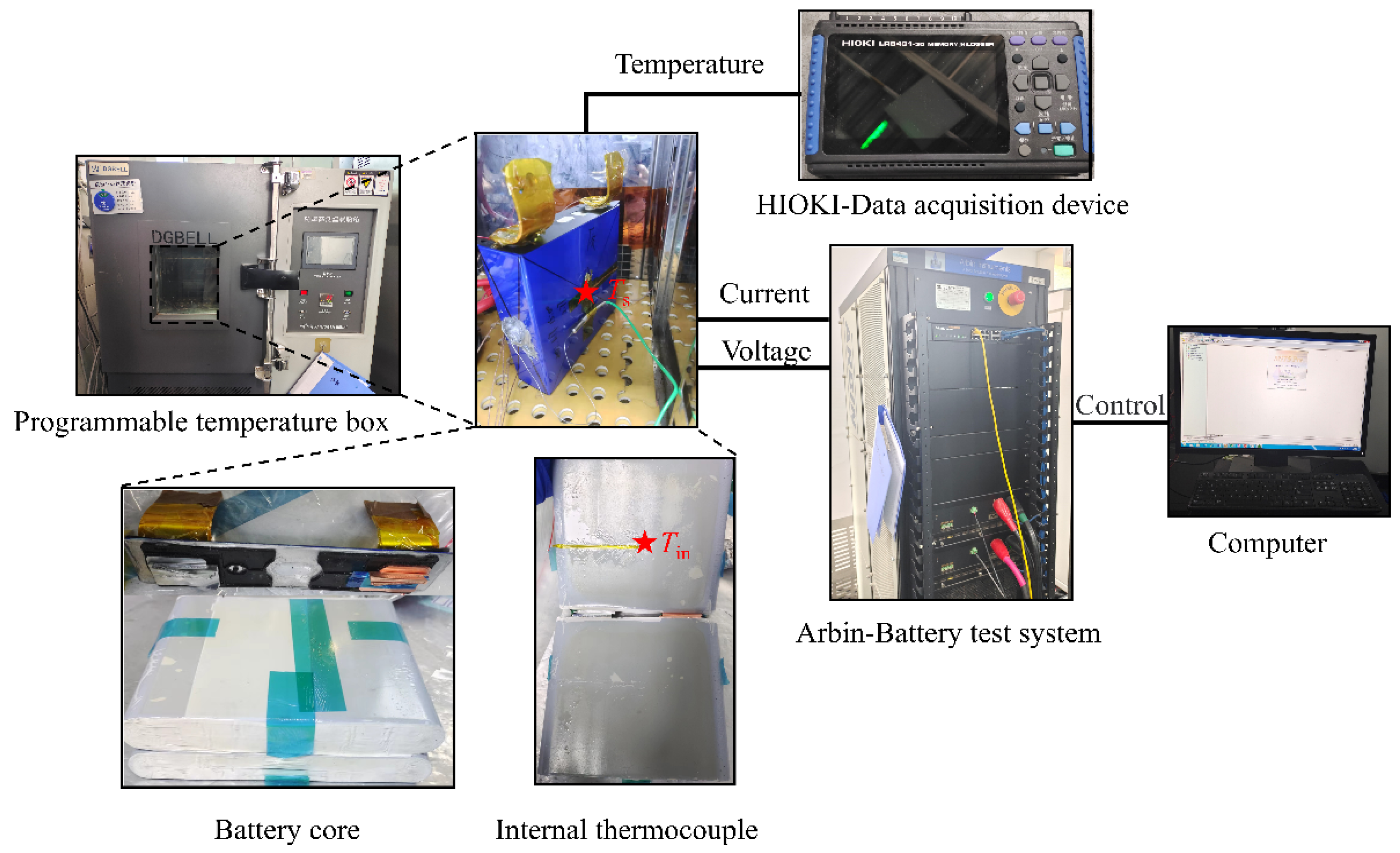
2.1. Battery Experiment

This research utilizes a 120 Ah commercial LiFePO4 battery. The typical parameters of the battery are shown in Table 1.
The experimental platform of the battery is illustrated in Figure 2. The charge/discharge system used in this study is produced by Arbin Instruments, College Station, TX, USA. It has a maximum testing current of 300 A and a maximum measurement voltage of 5 V. The charge/discharge unit is connected to the main control computer through controller area network (CAN) communication. Various experimental procedures can be performed on the battery by loading different test steps into the main control computer. The battery is placed inside a Bell BE-THK programmable temperature chamber to offer different environmental temperatures. The temperature chamber is manufactured by Bell Experiment Equipment Co., Ltd. in Dongguan, China. A K-type thermocouple is placed in the battery to obtain internal temperature data. The temperature is collected using a HIOKI data acquisition device. For detailed experimental procedures regarding the placement of the internal thermocouple, please refer to Supplementary Material Figure S1.
To obtain the basic characteristics of the battery, various experiments are conducted. The experimental content and main experimental steps are shown in Table 2. The battery capacity experiment aims to obtain the battery’s standard capacity. The capacity experiment value at 25 °C is 127.64 Ah. Actually, we have also conducted capacity experiments on the battery at 35 °C. The average capacity value from three 1/3C constant current discharges is 127.91 Ah, with a difference of only 0.2% compared to the capacity experiment at 25 °C. The difference in capacity is minimal. In the subsequent studies, the battery operates between 25 °C and 35 °C. Therefore, we neglected the influence of temperature on the capacity parameters. The HPPC tests are conducted at both 25 °C and 35 °C. Multiple-rate pulses of 1/3C, 1/2C, and 1C are applied. The transient voltage variations during the pulse segments support the identification of ECM parameters. In the HPPC experiments, pulse tests are conducted at every 5% SOC, allowing for voltage responses of the battery at more SOC points compared to tests conducted at every 10% SOC. Through parameter fitting methods, more densely distributed ECM parameters are obtained, resulting in more accurate parameter interpolation. As a result, the battery’s characteristics are better represented. To investigate the hysteresis characteristics of the battery, a main hysteresis experiment and two minor hysteresis experiments are conducted at 25 °C and 35 °C. The main hysteresis experiment aims to obtain the complete OCV hysteresis loop. The minor hysteresis experiments set different SOC variation paths to simulate the repetitive changes occurring in FR scenarios. We adjust the SOC by 5% by charging or discharging the battery at a current of 1/3C for 9 min. After adjusting the SOC, we let the battery rest, during which the current becomes zero. We measure the OCV value after a 3 h resting period. To establish a thermal model for the battery, tests are conducted to measure the entropy heat coefficient and multi-rate constant current experiments with the internal thermocouple. The accuracy of the two-state thermal model and the internal temperature estimation method is validated using experimental data. Finally, we conducted experiments under FR working conditions based on the FR commands from the Pennsylvania-New Jersey-Maryland Interconnection (PJM) electricity market from 4 July to 5 July 2020. The original FR commands range from −1 to 1. This value is multiplied by the battery’s rated power of 192 W and divided by the nominal voltage to obtain the dynamic current that the battery needs to respond to under the FR command. It is worth noting that experimental item 5 in Table 2 is conducted with the inserted thermocouple, while the other experiments are conducted without the inserted thermocouple. Before inserting the thermocouple, the battery is discharged to 0% SOC, and its OCV is measured as 2.83 V. After inserting the thermocouple, the battery is left to rest, and the OCV is measured again, resulting in the same value of 2.83 V. Due to the thermocouple’s small diameter of only 0.5 mm, the insertion of the thermocouple has no noticeable impact on the measurement of the OCV before and after its installation. The experimental results of the HPPC experiment, main hysteresis experiment, minor hysteresis experiment, and battery entropy heat experiment are shown in Figure 3.

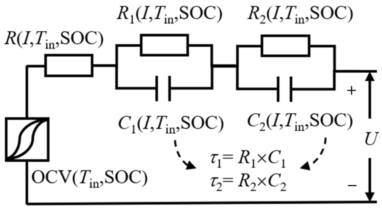
2.2. Second-Order RC Equivalent Circuit Model with Hysteresis Voltage Reconstruction

This study chose a second-order RC equivalent circuit model (SRCM) for electrical modeling. For hysteresis modeling, a hysteresis voltage reconstruction model (HVRM) is selected to describe the hysteresis characteristics of the battery. The electrical-hysteresis coupling schematic diagram is shown in Figure 4.

2.2.1. Hysteresis Voltage Reconstruction

The OCV of LiFePO4 batteries exhibits hysteresis characteristics related to the charging and discharging paths. As shown in Figure 3c, when the battery’s SOC changes from 0 to 1 during a unidirectional charge, its OCV value is higher than when the SOC changes from 1 to 0 during a unidirectional discharge. The area enclosed by the OCV curves during charge and discharge represents the possible OCV values of the battery during other SOC operating paths. Figure 3d shows the OCV of the battery with its SOC following the working path of 1→0.2→0.8→0.2→1. When the battery undergoes unidirectional continuous discharge from SOC 1 to 0.2 and 0.2 to 1, the OCV closely follows the main discharge hysteresis voltage curve and the main charge hysteresis voltage curve, respectively. However, when the battery undergoes bidirectional continuous charge and discharge from SOC 0.2 to 0.8 and back to 0.2, the OCV exhibits a loop-like variation. Figure 3e represents the OCV variation of the battery as the SOC changes along the path 1→0.4→0.6→0.4→1. The OCV behavior follows a similar pattern in Figure 3d. Furthermore, at both 25 °C and 35 °C, the OCV behavior during the hysteresis loop remains consistent, with slight variations in the measured OCV values. It is worth noting that prior to conducting the 35 °C hysteresis experiment, the battery is charged to full capacity at 25 °C using a CCCV method of 1/3C. Subsequently, the temperature box is adjusted to raise the temperature to 35 °C. This adjustment takes into consideration both the transition time required for the temperature box from 25 °C to 35 °C and the battery’s adaptation to the 35 °C environment. As a result, we allocate a resting time of 5 h for 1 SOC at 35 °C, allowing sufficient time for the battery to stabilize. The extended resting period at 35 °C leads to a lower OCV value for 1 SOC compared to the OCV value at 25 °C. The hysteresis OCV reconstruction equations approximate the OCV to the main hysteresis charging voltage curve during charging and the main hysteresis discharging voltage curve during discharging. These equations are shown as Equations (1) and (2).
d O C V h d z = d O C V c d z + δ O C V c O C V h , d z d t > 0 d O C V d i s d z + δ O C V h O C V d i s , d z d t 0
O C V h , t = O C V h , t 1 + O C V c , t O C V c , t 1 + δ ( O C V c , t 1 O C V h , t 1 ) ( z t z t 1 ) , d z d t > 0 O C V h , t 1 + O C V d i s , t O C V d i s , t 1 + δ O C V h , t 1 O C V d i s , t 1 z t z t 1 , d z d t 0
where O C V h , t represents the hysteresis OCV, where the subscript h indicates hysteresis and t represents time. O C V c represents the main hysteresis charging voltage, with the subscript c indicating charging, while O C V d i s represents the main hysteresis discharging voltage, with the subscript dis indicating discharging. δ denotes the correction factor, and z represents the state of charge (SOC).
The reference [16] had set the value of δ as 10. To determine the appropriate value of δ in our study, we conduct a parameter scan with increments of 0.1 within the range of 5 to 15. We find that the best fitting accuracy for the hysteresis OCV is achieved when δ is set to 13.8, as shown in Figure 5. At 25 °C, the root mean square error (RMSE) on minor hysteresis experiment-I is 3.4 mV, and on minor hysteresis experiment-II is 2.5 mV. At 35 °C, the RMSE on minor hysteresis experiment-I is 8.5 mV, and on minor hysteresis experiment-II is 3.3 mV.

2.2.2. Second-Order RC Equivalent Circuit Model

As shown in Figure 4, the polarization phenomenon of the battery is described using an SRCM. The ohmic resistance corresponds to the polarization of ion conduction in the electrolyte and electron conduction in the electrode material. The concentration and electrochemical polarization during the charge and discharge processes are described using two parallel branches of resistors and capacitors. According to simulation results from the literature [13], increasing the number of RC parallel networks beyond 2 does not significantly improve the accuracy of terminal voltage simulation. On the other hand, if the number of RC parallel networks is less than 2, there is a significant decrease in the accuracy of terminal voltage simulation. Therefore, in this study, we established an ECM with two RC parallel networks. The voltage equations are shown as (3)–(5). Unlike the traditional SRCM, the OCV is simulated using the above hysteresis voltage reconstruction equation. The parameters in the model vary with SOC, temperature, and current rate. To identify the parameters in the SRCM, HPPC experiments are conducted at 25 °C and 35 °C. The HPPC pulse rates chosen are 1/3C, 1/2C, and 1C, as shown in Figure 3a,b. Using the PSO algorithm [39], the parameters of the model, including the charge-discharge ohmic resistance, polarization capacitance, and time constant, are optimized to minimize the RMSE between the model’s simulated terminal voltage and the measured pulse segment voltage, as shown in Equation (6). The parameter identification results are illustrated in Figure 6. Temperature has a significant influence on the discharging ohmic resistance ( R d i s ) and charging ohmic resistance ( R c h a r ). As the temperature increases, the resistance decreases, while in the low SOC region, the resistance significantly increases. The polarizing capacitance C 1 and time constant τ 1 do not exhibit a clear pattern with temperature variations. However, the polarizing capacitance C 2 and time constant τ 2 increase with higher temperatures. The identification result of τ 2 is greater than τ 1 , indicating that the first parallel RC branch represents a faster electrochemical reaction polarization, while the second parallel RC branch represents a slower concentration polarization.
U i = I R i 1 e t τ i , i = 1 , 2
τ i = R i × C i , i = 1 , 2
U t = O C V h , t + I R + U 1 + U 2
R M S E = 1 N t = 1 N ( U t U m , t )
where U i represents the voltage across the i-th parallel RC branch, I represents the current (positive for charging), R is the Ohmic resistance, R i is the polarization resistance, C i is the polarization capacitance, τ i is the time constant of the parallel RC branch, U t represents the simulated voltage at time t, N is the number of voltage sampling data, and U m , t represents the measured voltage.

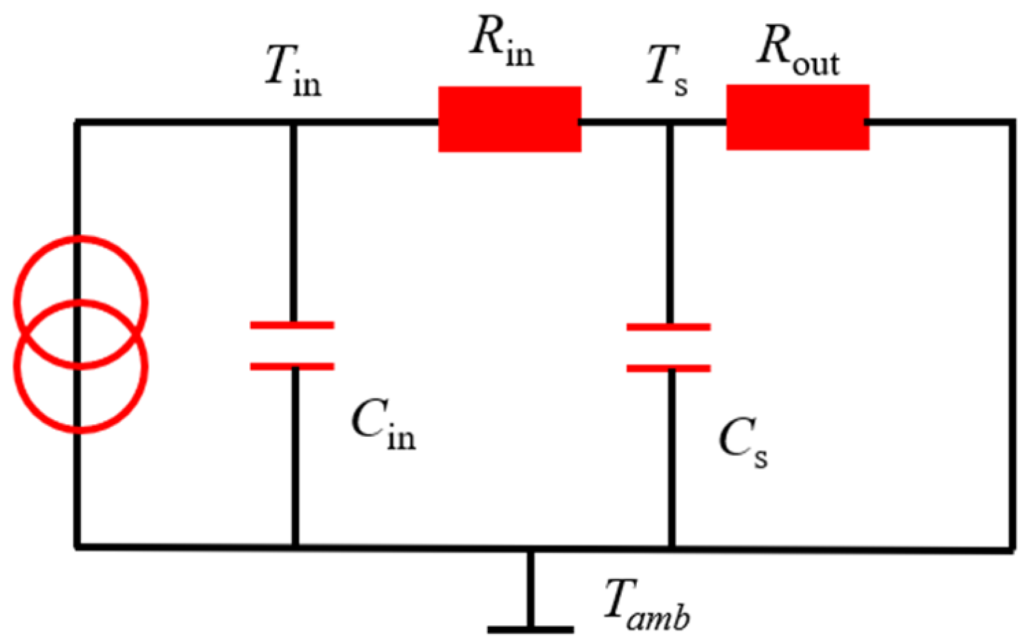
2.3. Estimation of Battery Core Temperature

2.3.1. Two-State Thermal Model

During the charge and discharge process of LiFePO4 batteries, heat is generated due to the polarization process, leading to an increase in internal temperature. The parameters of the equivalent circuit model vary with temperature. To accurately sense the temperature rise inside the battery, a two-state lumped parameter thermal model is constructed considering both the surface temperature and internal core temperature of the battery. The model is shown in Figure 7.
The model assumes that the heat generation in the battery consists of two components: Joule heating and reaction heat, as shown in Equation (7). The first heat generation component depends on the battery’s current and the hysteresis OCV. The second component depends on the current and the entropy potential. The entropy potential is calibrated through experiments and obtained by calculating the derivative of the OCV to temperature. The results are shown in Figure 3f. The heat transfer equation from the battery core to the casing is represented by Equation (8). The internal thermal resistance is the parallel combination of three directional resistances, as shown in Equation (9). In this study, the battery width is set as the w-direction, the height as the h-direction, and the length as the l-direction. The formulas for calculating the three directional thermal resistances are given by Equations (10)–(12). The heat dissipation from the battery casing to the environment is a convective heat transfer process, and the heat transfer is described by Equation (13). The external thermal resistance of the battery is related to the convective heat transfer coefficient, and its calculation formula is given by Equation (14). The thermal conductivity, specific heat capacity, and other parameters are provided by the battery manufacturer, and the main parameters in the thermal model are listed in Table 3. It is worth noting that the battery’s participation in FR services should occur at an optimal temperature range to prevent accelerated degradation in both low and excessively high temperature conditions. Additionally, since the ambient temperature remains relatively close to the battery temperature, the development of the thermal model disregards the impact of thermal radiation.
Q = ( O C V h , t U t ) × I + I T a b s d O C V h , t d T
C i n T i n t = Q T i n T s R i n
where Q represents the heat generation in the battery core, T a b s is the absolute temperature, d T is the temperature change, T i n is the internal temperature change, t is the data sampling time (1 s in this study), C i n is the specific heat capacity of the battery core, provided by the manufacturer, and R i n is the internal thermal resistance.
R i n = 1 1 R w + 1 R h + 1 R l
R w = L w λ w L l L h
R h = L h λ h L l L w
R l = L l λ l L h L w
where R w , R h , R l represent the thermal resistances in the width, height, and length directions, respectively. λ w , λ h , λ l represent the thermal conductivity coefficients in the width, height, and length directions, respectively, which are provided by the manufacturer. L l , L w , L h denote the length, width, and height of the battery, respectively, with specific values listed in Table 1.
C s T s t = T i n T s R i n T s T a m b R s
R s = 1 W × 2 × ( L l L h + L l L w + L h L w )
where C s represents the specific heat capacity of the casing, T s is the surface temperature, T a m b is the ambient temperature, R s is the external thermal resistance, and W is the convective heat transfer coefficient.
The experimental environment of this study is the same as that of reference [17], and the convective heat transfer coefficient W is set as 5 according to the setting of the reference.

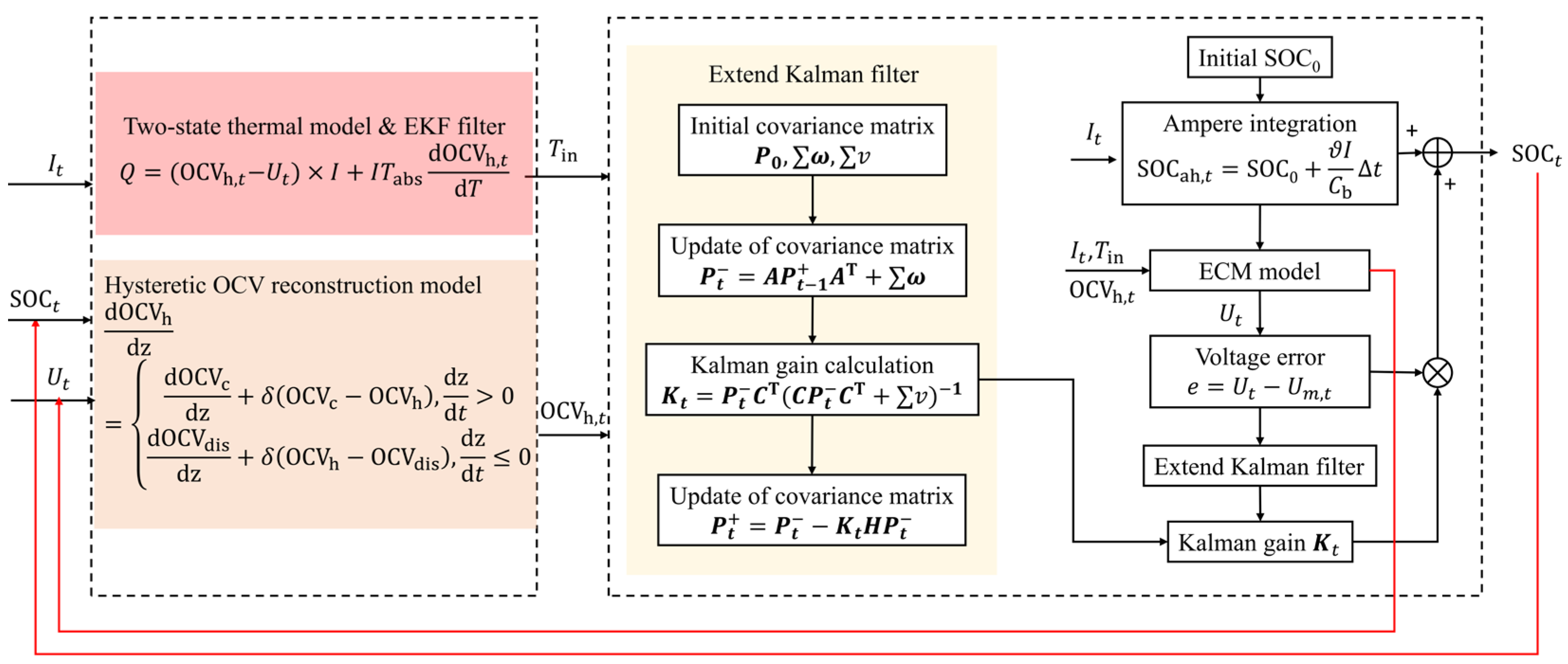
2.3.2. Battery Core Temperature Estimation Based on the Extended Kalman Filter (EKF) Algorithm

Using an embedded thermocouple to measure the internal temperature of a LiFePO4 battery is a destructive method that can compromise the internal structure of the battery. To ensure the safety of battery operation, it is generally not allowed to implant the thermocouple during the normal operation of the battery. Obtaining the internal temperature of a LiFePO4 battery during normal operation is challenging. The two-state thermal model is discretized to estimate the internal temperature in real-time, and a state-space equation is established, as shown in Equations (15)–(23). In the state equation, it is assumed that both the process noise and sampling noise follow a normal distribution. Based on the established two-state thermal model state equation, the Extended Kalman Filter (EKF) algorithm is used to correct the estimated internal temperature based on the error between the battery’s simulated and measured surface temperatures. The EKF algorithm can achieve optimality in the least squares sense and is widely used in modern control fields. The algorithm flow is shown in Table 4.
x t = A x t 1 + B u t 1 + ω t 1
y t = C x t + ν t
x t = [ T i n , t , T s , t ] T
u t 1 = Q t 1
A = 1 1 R i n C i n 1 R i n C i n 1 R i n C s 1 1 R i n C s 1 R o u t C s
B = [ 1 C i n , 0 ] T
C = [ 0   1 ]
E ω n ω t T = ω , n = t         0 , n t
E v n v t T = v , n = t         0 , n t
where x t represents a two-dimensional vector consisting of the internal temperature T i n , t and the surface temperature T s , t of the battery. y t represents the output of the battery’s surface temperature. u t 1 is the input, which is the heat generation in the battery core. ω t 1 represents the process noise, assumed to follow a normal distribution with a covariance of ω . ν t represents the sampling noise, also assumed to follow a normal distribution with a covariance of v . A B , C are state parameter transition matrices.
In the table, P 0 represents the initial covariance matrix, x ^ t represents the prior estimate of the state variable, x ^ t + represents the posterior estimate of the state variable, K t represents the Kalman gain matrix, and T s , m represents the measured surface temperature.
The covariance values are as follows:
P 0 = 10 3 0 0 10 3
ω = 10 3 0 0 5 × 10 3
v = 10 2
At an ambient temperature of 25 °C, constant current charge and discharge tests are conducted on the battery at current rates of 1/3C, 1/2C, and 1C to verify the accuracy of the internal temperature estimation based on the EKF algorithm using the two-state thermal model. The results of the internal and surface temperatures of the battery are shown in Figure 8. The RMSEs for the simulation of internal and surface temperatures are shown in Table 5. The measured internal temperature values are obtained using the embedded thermocouple. The battery surface temperature estimation errors are all less than 0.01 °C under the three operating conditions, indicating a very high estimation accuracy. This is because the correction effect of the EKF algorithm relies on the error between the estimated surface temperature and the measured value. When there is a large error in the estimated surface temperature, a larger Kalman gain is generated to bring the estimated surface temperature closer to the true value. The estimation error of the internal temperature increases with higher rates of charge/discharge. At a 1C rate, the RMSE of the internal temperature estimation is 0.75 °C. At a 1/2C rate, the RMSE of the internal temperature estimation is 0.39 °C. At a 1/3C rate, the RMSE of the internal temperature estimation is 0.22 °C. The temperature simulation error is less than 1 °C for all three operating conditions, indicating the method has accuracy in estimating the internal temperature.

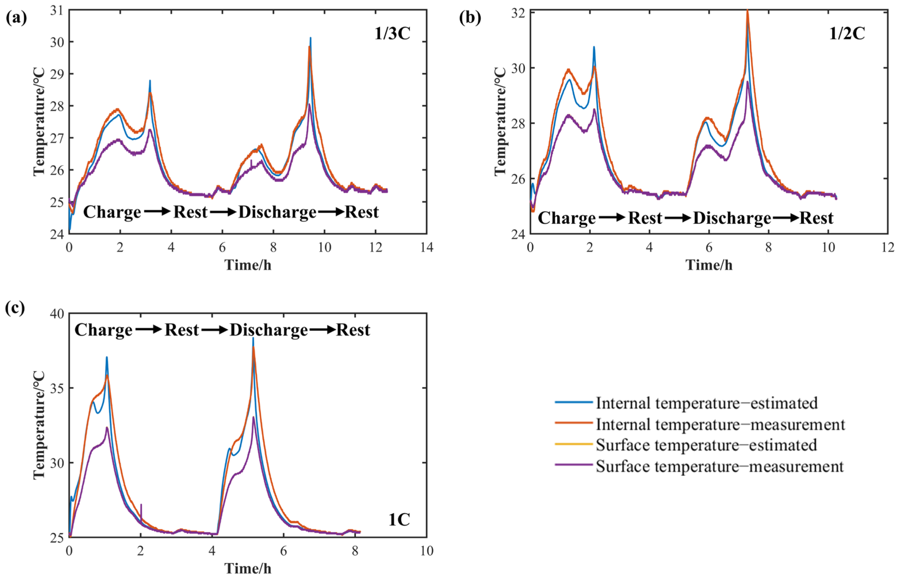
2.4. Terminal Voltage Simulation under Dynamic Frequency Regulation Working Conditions Using the Thermal-Electrochemical Coupling Model

To establish an accurate voltage model for LiFePO4 batteries, a coupled thermal-electric-hysteresis model is constructed by incorporating OCV hysteresis and internal temperature rise with the SRCM. This coupled model simulates the terminal voltage under dynamic FR working conditions. Real FR commands from two selected days in the PJM electricity market are chosen to verify the model’s accuracy. These commands are converted into current excitation by dividing the rated power of 192 W by the nominal voltage. Under FR working conditions, the current exhibits complex variations, including bidirectional pulses and high-frequency fluctuations. The algorithm framework of the thermal-electric-hysteresis coupled model is shown in Figure 9. Firstly, the current under FR working conditions is obtained, as shown in Figure 10a. The reconstructed OCV is calculated using the HVRM. This OCV is then input into the two-state thermal model to calculate the heat generation. The EKF algorithm is utilized to achieve an optimal internal temperature estimation. The obtained internal temperature value, along with the current rate interpolation, is used to obtain the parameters of the ECM. Finally, the terminal voltage is calculated. The terminal voltage is fed back into the two-state thermal model, and the iteration process continues, enabling real-time calculation of the internal temperature, hysteresis OCV, and internal temperature. The voltage simulation results of the thermal-electric-hysteresis coupled model under FR working conditions are shown in Figure 10e, while the simulation error of the terminal voltage is shown in Figure 10f. Under this operating condition, the battery’s internal temperature is approximately 2 °C higher than the surface temperature, as shown in Figure 10b. The RMSE between the simulated surface temperature of the battery and the estimated temperature is 0.0024 °C. The high-accuracy simulation is achieved due to the strong corrective effect of the EKF algorithm, which utilizes surface temperature error information for robust correction. The OCV repeatedly varies diagonally within the main hysteresis voltage curve, and a single OCV curve alone cannot capture this variation, as shown in Figure 10c,d. Under the nearly 48 h FR working condition, the RMSE of the voltage is only 18.7 mV, indicating that the model has high simulation accuracy and can be used for subsequent SOC and RAE estimation methods.

3. SOC and RAE Estimation under Dynamic Frequency Regulation Working Condition

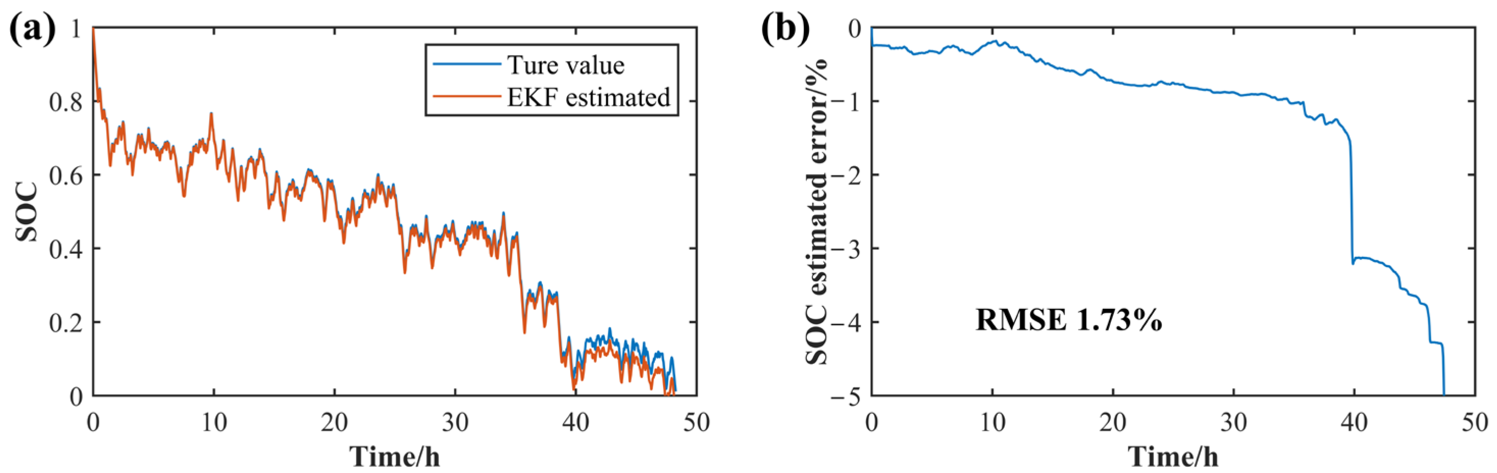
3.1. SOC Estimation Based on the EKF Algorithm

Using the ampere-hour integration method to calculate SOC, as shown in Equation (30), this method is affected by factors such as current sampling noise and inaccurate initial SOC, resulting in inaccurate SOC estimation. Therefore, the established thermal-electric-hysteresis voltage model is used to create a state equation, and the EKF algorithm is employed for closed-loop feedback correction of SOC obtained through the ampere-hour integration method. The state variables, state outputs, and state transition matrix are shown in Equations (31)–(35). The flowchart of estimating SOC using the EKF algorithm is shown in Figure 11.
The covariance values are as follows:
P 0 = 10 5 0 0 0 0 0 0 0 0
ω = 2 × 10 10 0 0 0 0 0 0 0 0
v = 0.1
S O C a h , t = S O C 0 + ϑ I C b t
where S O C a h , t represents the SOC value calculated through the ampere-hour integration method, S O C 0 is the initial SOC value, which is set to 1 in this study. C b represents the battery’s rated capacity, which is 127.64 Ah. ϑ represents the Coulomb efficiency, which is set to 1. t represents the sampling time interval, which is 1 s in this study.
x t = [ S O C a h , t U 1 , t U 2 , t ]
y t = U t
A = 1 0 0 0 e t τ 1 0 0 0 e t τ 2
B = [ t 3600   ×   C b R 1 ( 1 e t τ 1 ) R 2 ( 1 e t τ 2 ) ] T
C = [ d O C V h , t d S O C 1 1 ]
where x t represents the state vector, and y t represents the output value. U 1 , t and U 2 , t represent the polarization voltages of the two RC elements, and U t represents the terminal voltage output of the thermal-electric-hysteresis coupling model.
It is worth noting that in this study, the OCV is calculated using the HVRM. In matrix C, the derivative of the hysteresis OCV to SOC is considered. This is different from the EKF algorithm based on traditional ECM models. Meanwhile, the model parameters, such as resistance, are interpolated based on internal temperature, which differs from the traditional surface temperature interpolation method. Due to the high-frequency variations in the OCV under FR working conditions, significant Kalman gains are generated to correct SOC estimation errors continuously. The true values of SOC are obtained through the method of ampere-hour integration, under the condition of high-precision laboratory current sensing equipment and accurate initial SOC value settings. This algorithm exhibits high SOC estimation accuracy under FR working conditions, as demonstrated by the SOC estimation results in Figure 12a,b, with an RMSE of only 1.73%.

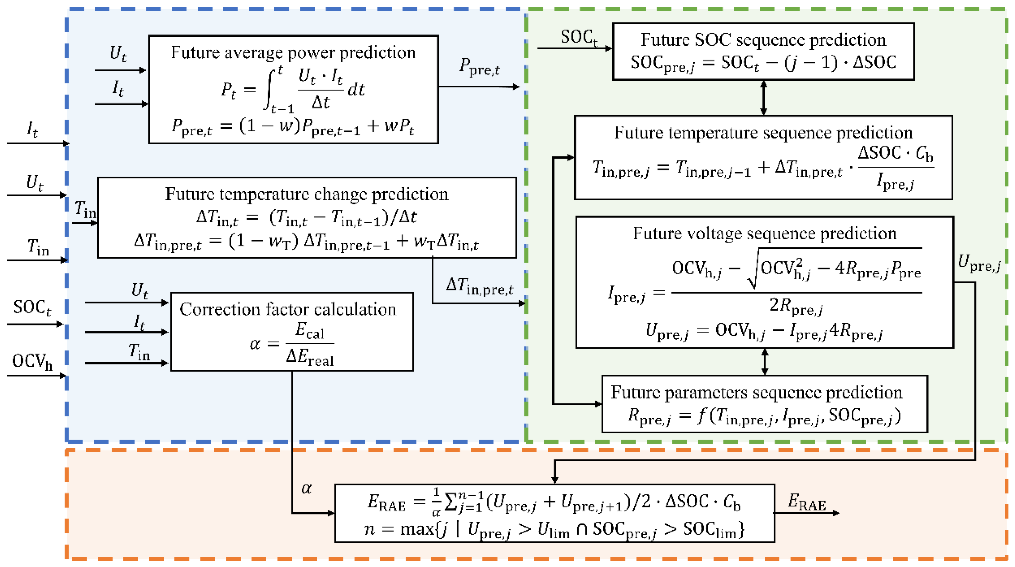
3.2. RAE Estimation Algorithm Based on Future Voltage Sequence Prediction

Battery’s RAE prediction refers to estimating the actual energy that a battery can deliver when discharged from its current state to the cutoff voltage under a specific operational condition. In FR working conditions, the relevant factor affecting the functional state of the battery is the RAE of the battery rather than the remaining theoretical energy. Therefore, based on practical application requirements, the estimation of the battery’s RAE is studied. The approach to studying this problem is illustrated in Figure 13. At a particular moment in this operational condition (indicated by the green vertical line), the curve on the left represents the variation of historical terminal voltages measured to SOC. On the right side, there is a curve representing the predicted future terminal voltages. If the area enclosed by the voltage curve and the x-axis is divided into intervals based on certain SOC increments, and for each ∆SOC interval, a future terminal voltage U p r e , j is predicted, then the RAE E 1 corresponding to the light orange region can be approximated as ( U p r e , 1 + U p r e , 2 ) / 2 × S O C × C b . Therefore, the current remaining discharge energy can be calculated using Equation (36).
E R A E j = 1 n 1 ( U p r e , j + U p r e , j + 1 ) / 2 × S O C × C b
where E R A E represents the RAE at the current time, U p r e , j represents the future terminal voltage sequence, and n represents the discharge cutoff point.
Based on Equation (36), it can be analyzed that the accurate estimation of RAE relies on predicting the future terminal voltage sequence, which is influenced by future operational conditions and changes in internal battery temperature. Therefore, based on known historical operating conditions and data such as current, voltage, and internal temperature, it is necessary to predict future FR power and future internal battery temperature. On this basis, the future voltage can be predicted based on the battery model. Since the battery model parameters are directly related to SOC and temperature, combining the current SOC estimation and parameter identification results is necessary to couple predict the future SOC sequence, future internal battery temperature sequence, future model parameter sequence, and future terminal voltage sequence. Finally, the remaining discharge energy can be calculated by considering the determination of the discharge cutoff point. Specifically, it includes the following three key steps: (1) Future operational condition prediction, including future average power prediction and future internal battery temperature prediction; (2) Coupled prediction of future SOC sequence, future internal battery temperature sequence, future terminal voltage sequence, and future parameter sequence; (3) Discharge cutoff point determination and estimation of RAE.

3.2.1. Future Operational Condition Prediction Based on Historical Information

This research uses a schedule according to FR commands with a rated power of 192 W. In practical scenarios, the battery’s power in FR conditions constantly varies. To mitigate the impact of frequent fluctuations in instantaneous power on power predictions while ensuring that the power predictions can track the changes in actual operating conditions, a moving weighted average of historical power is computed as the prediction for future power. This is represented by Equations (37) and (38).
P t = t 1 t U t · I t t d t
P p r e , t = 1 w P p r e , t 1 + w P t
where P t represents the average power during the time interval from time t 1 to t . The calculation is assumed to be performed every time 12 Wh of energy is discharged. P p r e , t denotes the predicted value of future average power. The weight factor w is introduced to enhance the influence of the current moment on future operational conditions. FR working conditions refer to operational scenarios characterized by bidirectional high-frequency variations. In these conditions, the battery state undergoes frequent changes at each moment. Hence, we assign a higher weight to the current state to emphasize its impact on future predictions. Therefore, the weight factor w is set to 0.9.
Due to factors such as the battery’s self-heating and ambient temperature changes, the internal temperature of the battery varies during future discharge processes. This will further impact the magnitude of the RAE. Therefore, it is necessary to predict the future temperature changes. Similar to the approach used for power prediction, historical temperature changes are employed to forecast future temperature changes, as shown in Equations (39) and (40).
T i n , t = ( T i n , t T i n , t 1 ) / t
T i n , p r e , t = ( 1 w T )   T i n , p r e , t 1 +   w T T i n , t
where T i n , t represents the average internal temperature change during the time interval from time t 1 to t . The calculation is assumed to be performed every time 12 Wh of energy is discharged. T i n , p r e , t denotes the predicted value of future internal temperature. The weight factor w T is introduced to enhance the influence of the current moment on future temperature changes. In this research, w T is set to 0.9.

3.2.2. Model-Based Future Voltage Prediction

Based on the predicted future FR power values, it is possible to forecast future voltage using the battery model. Since the model parameters are related to current, SOC, and internal temperature, it is necessary to couple the prediction of future model parameters, future SOC, and future internal temperature to obtain the future voltage sequence. Starting from the current S O C t , the future discharge process is divided into segments with a certain SOC interval. The future SOC sequence S O C p r e , j is calculated according to Equation (41). The interval S O C can be set based on practical needs. A smaller S O C leads to a denser future voltage sequence and, theoretically, more accuracy. However, it also results in a higher computational load. In this research, S O C is set to 0.01.
S O C p r e , j = S O C t ( j 1 ) · S O C
where S O C p r e , j represents the future SOC sequence, where j denotes the index of the sequence point.
If the current temperature of the battery is T i n , t and the predicted future temperature change rate is T i n , p r e , t , then according to Equation (42), the future temperature change sequence T i n , p r e , j can be calculated. Here, I p r e , j 1 represents the predicted future current value and the prediction method for the future current will be provided in the following context.
T i n , p r e , j = T i n , t , j = 1 T i n , p r e , j = T i n , p r e , j 1 + T i n , p r e , t · S O C · C b I p r e , j 1
where T i n , t represents the current temperature, T i n , p r e , t represents the predicted future internal temperature change rate, and I p r e , j 1 represents the predicted future current value.
If we use an SRCM to predict future voltage, it will introduce significant computational complexity. The output power is calculated based on the Rint model to reduce the complexity of the model. Equations (43)–(46) show the future voltage prediction.
P p r e = ( O C V h , j I p r e , j R p r e , j ) I p r e , j
R p r e , j I p r e , j 2 O C V h , j I p r e , j + P p r e = 0
I p r e , j = O C V h , j O C V h , j 2 4 R p r e , j P p r e 2 R p r e , j
U p r e , j = O C V h , j I p r e , j R p r e , j
where P p r e represents the output power, O C V h , j represents the hysteresis OCV, I p r e , j represents the predicted current value, and R p r e , j represents the predicted value of future internal resistance parameters.
Considering that the SRCM is used in the SOC estimation algorithm of this research and predicting future voltage based on the average power is already an approximate estimation, there is no additional calibration of the Rint model parameters. The resistance value in the Rint model is substituted with the ohmic resistance from the SRCM, as shown in Equation (47). This resistance parameter is correlated with the future internal temperature, current, and SOC.
R p r e , j = f ( T i n , p r e , j , I p r e , j , S O C p r e , j )

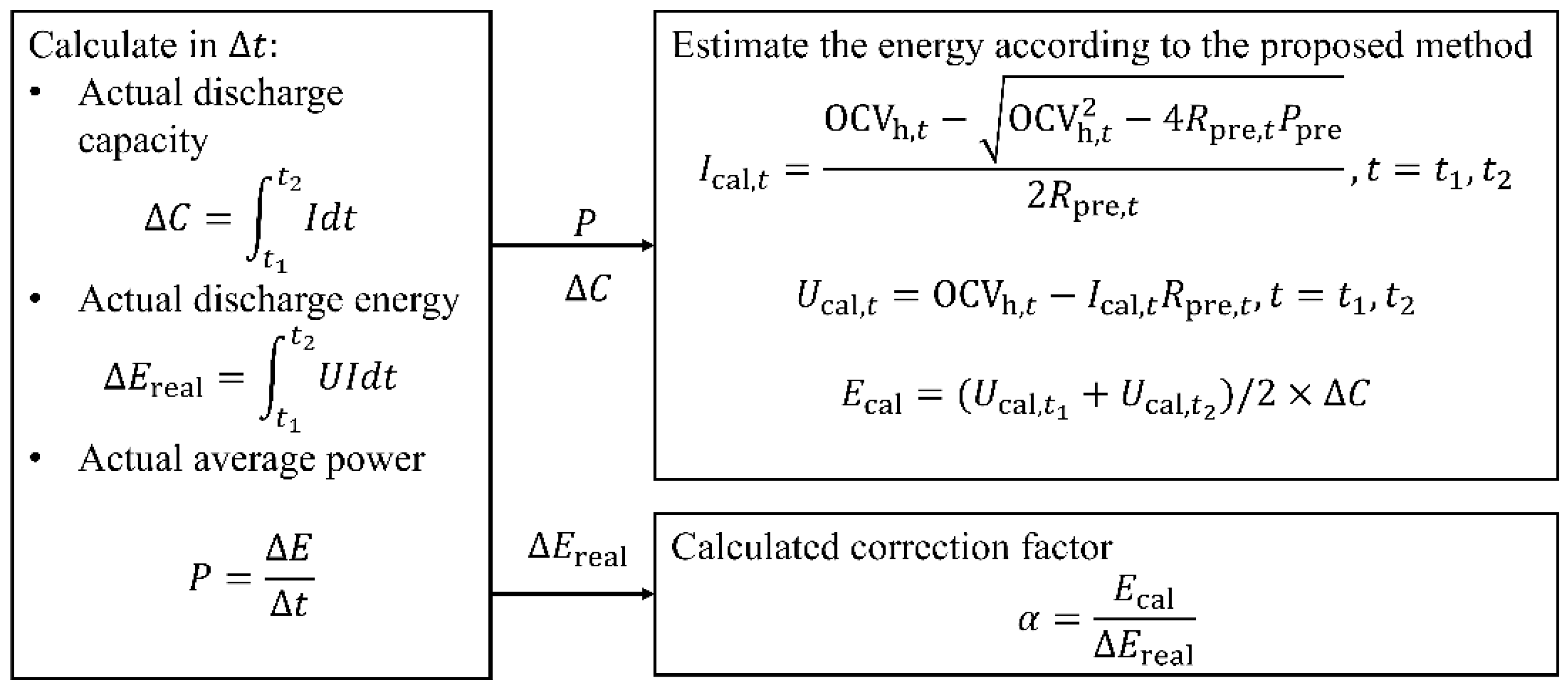
3.2.3. Determination of Discharge Cutoff Point and Estimation of RAE

To accurately estimate the RAE after obtaining the predicted future voltage sequence, it is necessary to determine the battery’s discharge cutoff point. The battery discharge cutoff is determined based on two criteria: first, when the voltage reaches the lower cutoff voltage of 2.5 V, and second, when the battery reaches 0 SOC. With the predictions mentioned above of future voltage and the determination of the discharge cutoff point, the RAE of the battery can be estimated using Equation (48), where the determination of the discharge cutoff point, denoted as ‘n’, satisfies Equation (49).
E R A E = j = 1 n 1 ( U p r e , j + U p r e , j + 1 ) / 2 · S O C · C b
n = m a x { j U p r e , j > U l i m S O C p r e , j > S O C l i m }
where E R A E represents the RAE at the current time, U p r e , j is the predicted future voltage sequence, n represents the discharge cutoff point, U l i m is the discharge cutoff voltage with a value of 2.5, and S O C l i m is the cutoff SOC value of 0.
However, when using Equation (48) to predict the RAE, there may be some errors, which mainly arise from the following sources:
(1)
The use of the ohmic resistance value from the SRCM.
(2)
The Rint model is relatively simple, and there may be errors when calculating future voltage based on predicted future power values.
(3)
Even if the voltage prediction is accurate, there is an inherent approximation error in approximating the area of the light orange shaded region in Figure 13 using ( U p r e , 1 + U p r e , 2 ) / 2 × S O C × C b .
It is important to be aware of these potential sources of error when using Equation (48) for predicting the remaining discharge energy.
This research proposes a correction method to improve the accuracy of estimating the RAE, as shown in Figure 14. The correction approach is as follows: between time t 1 and t 2 , estimate the energy using the method proposed in this research, and then divide it by the actual discharged energy to obtain the correction coefficient α . Taking into account the correction coefficient, the final estimation of the RAE is calculated using Equation (50). The complete process of estimating the RAE based on voltage prediction is illustrated in Figure 15. In Figure 15, the blue region represents the prediction method for future current and future internal temperature, as well as the calculation of correction factors. The green region represents the prediction of future physical quantity sequences. The orange region represents the calculation method for RAE.
E R A E = 1 α j = 1 n 1 ( U p r e , j + U p r e , j + 1 ) / 2 · S O C · C b
where α is correction coefficient.
The estimation results of RAE in dynamic FR working conditions are shown in Figure 16a,b. The error is defined as the predicted RAE subtracted from the real RAE, divided by the maximum available energy, as shown in Equation (51). The real RAE is calculated by integrating the reverse power after the battery has been completely discharged. The RMSE for the prediction of the RAE is 2.13%, which indicates that the algorithm has a very high estimation accuracy.
e t = E R A E , t E R A E , t u r e , t m a x ( E R A E , t u r e , t )
where e t represents the estimation error of the RAE, where E R A E , t is the estimated RAE, E R A E , t u r e , t is the true RAE obtained through reverse power integration after discharging, and m a x ( E R A E , t u r e , t ) represents the maximum value of the remaining available energy.

4. Conclusions

This research focuses on a 120 Ah commercial LiFePO4 battery and investigates its performance under dynamic FR working conditions. The research addresses the issues of poor voltage simulation accuracy due to neglecting hysteresis and internal temperature coupling effects in the ECM, as well as inaccurate estimation of SOC and RAE. To address these challenges, a novel method based on a thermal-electric-hysteresis model is proposed to evaluate SOC and RAE accurately.
LiFePO4 batteries exhibit hysteresis characteristics in their OCV. An HVRM is constructed based on main and minor hysteresis experimental data, accurately simulating the OCV values. The maximum RMSE of OCV simulation at 25 °C and 35 °C is 8.3 mV. A two-state thermal model considering surface and core temperatures is developed to estimate internal temperature. The core temperature is estimated using the closed-loop estimation approach with the EKF algorithm. The RMSE of internal temperature estimation under three constant current conditions is less than 1 °C. Based on the HPPC experiment data, the parameters of an SRCM under various temperatures and current rates are obtained using the PSO algorithm. A thermal-electric-hysteresis voltage simulation framework is established. The RMSE of voltage simulation under a dynamic FR working condition close to 48 h is only 18.7 mV. The developed thermal-electric-hysteresis model exhibits a very high level of accuracy.
Based on the thermal-electric-hysteresis model, the EKF algorithm is utilized to correct the initial value of SOC calculated through the ampere-hour integration method, enabling accurate estimation of SOC under FR working conditions. Furthermore, by utilizing future voltage prediction methods, accurate estimation of RAE under dynamic FR working conditions is achieved. The RMSE for SOC and RAE estimation is only 1.73% and 2.13%, respectively, indicating a very high level of estimation accuracy.
However, in this study, the simulation accuracy of terminal voltage under low temperature and high current rates working conditions for the proposed model has not been validated. Therefore, future research should consider further validation under these two scenarios. In these situations, it may be beneficial to explore online identification of ECM parameters or utilize an improved ECM to enhance the accuracy of terminal voltage simulation. Moreover, we use the temperature at the center point of the front surface of the battery casing to represent the variations in surface temperature. However, there are temperature gradients on the battery surface, and temperature sampling data from different locations on the surface may exhibit differences. The impact of surface temperature variations on battery state estimation needs further research and validation. Finally, the OCV experiment is not conducted on batteries with inserted thermocouples. Future work needs to further verify the consistency of OCV between batteries with inserted thermocouples and batteries without inserted thermocouples within the 0–1 SOC range.

Supplementary Materials

The following supporting information can be downloaded at: https://www.mdpi.com/article/10.3390/en16135239/s1, Figure S1: The detailed operating procedures of inserting thermocouple into the battery. Figure S2: The variation of OCV over time. Figure S3: 1/3C discharge voltage curve. Table S1. C1 parameter identification results @ 25 °C. Table S2. C1 parameter identification results @ 35 °C. Table S3. C2 parameter identification results @ 25 °C. Table S4. C2 parameter identification results @ 35 °C. Table S5. Rdis parameter identification results @ 25 °C. Table S6. Rdis parameter identification results @ 35 °C. Table S7. Rchar parameter identification results @ 25 °C. Table S8. Rchar parameter identification results @ 35 °C. Table S9. τ1 parameter identification results @ 25 °C. Table S10. τ1 parameter identification results @ 35 °C. Table S11. τ2 parameter identification results @ 25 °C. Table S12. τ2 parameter identification results @ 35 °C.

Author Contributions

Conceptualization, Z.Z. and L.L.; methodology, Z.Z. and L.L.; software, Z.Z.; validation, Z.Z.; formal analysis, Z.Z.; investigation, Z.Z.; resources, Z.Z.; data curation, Z.Z.; writing—original draft preparation, Z.Z.; writing—review and editing, Y.L.; visualization, Z.Z.; supervision, M.O. and H.W.; project administration, M.O.; funding acquisition, L.L., H.W., Y.L. and M.O. All authors have read and agreed to the published version of the manuscript.

Funding

This work is supported by the Ministry of Science and Technology of China (Grant No. 2022YFE0207700), and funded by China National Postdoctoral Program for Innovative Talents (grant no.BX20220171), China Postdoctoral Science Foundation (grant no. 2022M711760), Shuimu Tsinghua Scholar Program (grant no. 2021SM130), National Natural Science Foundation of China (Youth Program Grant No. 52207240), Shandong Province Science and Technology Foundation (Youth Program Grant No. ZR2022QE099), International Joint Mission On Climate Change and Carbon Neutrality, and sponsored by Tsinghua-Toyota Joint Research Fund.

Data Availability Statement

Not applicable.

Acknowledgments

The authors thank Chongqing Energy Storage Safety Technology Innovation Center Co., Ltd. for providing experiment batteries.

Conflicts of Interest

The authors declare no conflict of interest.

Nomenclature

Abbreviations
ItemDescription
FRFrequency regulation
LiFePO4Lithium iron phosphate
EVsElectric vehicles
SOCState of charge
RAERemaining available energy
OCVOpen-circuit voltage
NNMsNeural network models
P2DPseudo-two-dimensions
SPSingle particle
SP2DSimplified pseudo-two-dimensions
ROMReduced-order model
FUDSFederal urban driving schedule
DSTDynamic stress test
1DOne-dimensional
2DTwo-dimensional
3DThree-dimensional
EKFExtended Kalman filter
KFKalman filter
PFParticle filter
SOEState of energy
HVRMHysteresis voltage reconstruction model
HPPCHybrid Pulse Power Characterization
PSOParticle Swarm Optimization
MAPMulti-Dimensional Parameter
SRCMSecond-order RC equivalent circuit model
CANController area network
PJMPennsylvania-New Jersey-Maryland
CCConstant current
CCCVConstant current and constant voltage
RMSERoot mean square error
Symbols
ItemDescriptionUnit
O C V h Hysteretic open circuit voltage.V
O C V c Main hysteresis charging voltage.V
O C V d i s Main hysteresis discharging voltage.V
δ Correction factor./
zState of charge./
U i The voltage across the i-th parallel RC branch, i = 1, 2.V
ICurrent (positive for charging).A
R Ohmic resistance.Ω
R i Polarization resistance of the i-th parallel RC branch, i = 1, 2.Ω
C i Polarization capacitance of the i-th parallel RC branch, i = 1, 2.Ω
τ i Time constant of the i-th parallel RC branch, i = 1, 2.s
U t Simulated voltage at time t.V
NThe number of voltage sampling data./
U m , t Measured voltage.V
Q Heat generation in the battery core.W
T a b s Absolute temperature.°C
d T Temperature change.°C
T i n Internal temperature change.°C
t The data sampling time (1 s in this study).s
C i n The specific heat capacity of the battery core.J/(kg·K)
R i n The internal thermal resistance.K/W
R w The thermal resistances in the width direction.K/W
R h The thermal resistances in the height direction.K/W
R l The thermal resistances in the length direction.K/W
λ w The thermal conductivity coefficients in the width direction.W/(m·K)
λ h The thermal conductivity coefficients in the height direction.W/(m·K)
λ l The thermal conductivity coefficients in the length direction.W/(m·K)
L l The length of the battery.m
L w The width of the battery.m
L h The height of the battery.m
C s The specific heat capacity of the casing.J/(kg·K)
T s Surface temperature of the battery.°C
T a m b Ambient temperature.°C
R s External thermal resistance.K/W
WConvective heat transfer coefficient.W/(m2·K)
x t The state vector of the state-space equation./
y t The output vector of the state-space equation./
u t 1 The input vector of the state-space equation./
ω t 1 Process noise./
ν t Sampling noise./
A ,   B , C Parameter transition matrices./
P 0 Initial covariance matrix./
x ^ t The prior estimate of the state variable./
x ^ t + The posterior estimate of the state variable./
K t Kalman gain matrix/
T s , m The measured surface temperature.°C
S O C a h , t SOC value calculated through the ampere-hour integration method./
S O C 0 Initial SOC value./
ϑ Coulomb efficiency./
C b The battery’s rated capacity.Ah
E R A E Remaining available energy.Wh
U p r e , j The future terminal voltage sequence. j denotes the index of the sequence point.V
nThe discharge cutoff point./
P t Average power during the time interval from time t − 1 to t.W
P p r e , t The predicted value of future average power.W
w Weight factor./
T i n , t The average internal temperature change during the time interval from time t − 1 to t.°C
T i n , p r e , t Predicted value of future internal temperature change.°C
w T Weight factor of temperature./
S O C p r e , j The future SOC sequence.
T i n , t The internal temperature at time t.°C
T i n , p r e , t The predicted future internal temperature change.°C
I p r e , j 1 Predicted future current value.A
P p r e The predicted output power.Wh
I p r e , j The predicted current value.A
R p r e , j The predicted value of future internal resistance parameters.Ω
U p r e , j The predicted future voltage sequence.V
U l i m The discharge cutoff voltage.V
S O C l i m The discharge cutoff SOC./
α Correction coefficient./
e t The estimation error of the remaining available energy/
E R A E , t The estimated remaining available energyWh
E R A E , t u r e , t The true remaining available energy obtained through reverse power integration after dischargingWh

References

  1. Li, Y.; Wei, Y.; Zhu, F.; Du, J.; Zhao, Z.; Ouyang, M. The path enabling storage of renewable energy toward carbon neutralization in China. Etransportation 2023, 16, 100226. [Google Scholar] [CrossRef]
  2. Dixon, J.; Bukhsh, W.; Bell, K.; Brand, C. Vehicle to grid: Driver plug-in patterns, their impact on the cost and carbon of charging, and implications for system flexibility. Etransportation 2022, 13, 100180. [Google Scholar] [CrossRef]
  3. Hu, G.; Huang, P.; Bai, Z.; Wang, Q.; Qi, K. Comprehensively analysis the failure evolution and safety evaluation of automotive lithium ion battery. Etransportation 2021, 10, 100140. [Google Scholar] [CrossRef]
  4. Wang, X.; Wei, X.; Zhu, J.; Dai, H.; Zheng, Y.; Xu, X.; Chen, Q. A review of modeling, acquisition, and application of lithium-ion battery impedance for onboard battery management. Etransportation 2021, 7, 100093. [Google Scholar] [CrossRef]
  5. Xu, C.; Li, L.; Xu, Y.; Han, X.; Zheng, Y. A vehicle-cloud collaborative method for multi-type fault diagnosis of lithium-ion batteries. Etransportation 2022, 12, 100172. [Google Scholar] [CrossRef]
  6. Liu, Y.; Zhang, C.; Jiang, J.; Zhang, L.; Zhang, W.; Wang, L.Y. Deduction of the transformation regulation on voltage curve for lithium-ion batteries and its application in parameters estimation. Etransportation 2022, 12, 100164. [Google Scholar] [CrossRef]
  7. Doyle, M.; Fuller, T.F.; Newman, J. Modeling of galvanostatic charge and discharge of the lithium/polymer/insertion cell. J. Electrochem. Soc. 1993, 140, 1526. [Google Scholar] [CrossRef]
  8. Han, X.; Ouyang, M.; Lu, L.; Li, J. Simplification of physics-based electrochemical model for lithium ion battery on electric vehicle. Part I: Diffusion simplification and single particle model. J. Power Sources 2015, 278, 802–813. [Google Scholar] [CrossRef]
  9. Han, X.; Ouyang, M.; Lu, L.; Li, J. Simplification of physics-based electrochemical model for lithium ion battery on electric vehicle. Part II: Pseudo-two-dimensional model simplification and state of charge estimation. J. Power Sources 2015, 278, 814–825. [Google Scholar] [CrossRef]
  10. Rodríguez, A.; Plett, G.L.; Trimboli, M.S. Improved transfer functions modeling linearized lithium-ion battery-cell internal electrochemical variables. J. Energy Storage 2018, 20, 560–575. [Google Scholar] [CrossRef]
  11. Hu, X.; Feng, F.; Liu, K.; Zhang, L.; Xie, J.; Liu, B. State estimation for advanced battery management: Key challenges and future trends. Renew. Sustain. Energy Rev. 2019, 114, 109334. [Google Scholar] [CrossRef]
  12. Wang, Y.; Tian, J.; Sun, Z.; Wang, L.; Xu, R.; Li, M.; Chen, Z. A comprehensive review of battery modeling and state estimation approaches for advanced battery management systems. Renew. Sustain. Energy Rev. 2020, 131, 110015. [Google Scholar] [CrossRef]
  13. Hu, X.; Li, S.; Peng, H. A comparative study of equivalent circuit models for Li-ion batteries. J. Power Sources 2012, 198, 359–367. [Google Scholar] [CrossRef]
  14. Srinivasan, V.; Newman, J. Existence of path-dependence in the LiFePO4 electrode. Electrochem. Solid-State Lett. 2006, 9, A110. [Google Scholar] [CrossRef]
  15. Dreyer, W.; Jamnik, J.; Guhlke, C.; Huth, R.; Moškon, J.; Gaberšček, M. The thermodynamic origin of hysteresis in insertion batteries. Nat. Mater. 2010, 9, 448–453. [Google Scholar] [CrossRef]
  16. Huria, T.; Ludovici, G.; Lutzemberger, G. State of charge estimation of high power lithium iron phosphate cells. J. Power Sources 2014, 249, 92–102. [Google Scholar] [CrossRef]
  17. Mao, S.; Han, M.; Han, X.; Lu, L.; Feng, X.; Su, A.; Wang, D.; Chen, Z.; Lu, Y.; Ouyang, M. An Electrical–Thermal Coupling Model with Artificial Intelligence for State of Charge and Residual Available Energy Co-Estimation of LiFePO4 Battery System under Various Temperatures. Batteries 2022, 8, 140. [Google Scholar]
  18. Wang, Z.; Du, C. A comprehensive review on thermal management systems for power lithium-ion batteries. Renew. Sustain. Energy Rev. 2021, 139, 110685. [Google Scholar] [CrossRef]
  19. Wang, T.; Tseng, K.-J.; Yin, S.; Hu, X. Development of a one-dimensional thermal-electrochemical model of lithium ion battery. In Proceedings of the IECON 2013-39th Annual Conference of the IEEE Industrial Electronics Society, Vienna, Austria, 10–13 November 2013; pp. 6709–6714. [Google Scholar]
  20. Xu, M.; Zhang, Z.; Wang, X.; Jia, L.; Yang, L. Two-dimensional electrochemical–thermal coupled modeling of cylindrical LiFePO4 batteries. J. Power Sources 2014, 256, 233–243. [Google Scholar] [CrossRef]
  21. Ghalkhani, M.; Bahiraei, F.; Nazri, G.-A.; Saif, M. Electrochemical–thermal model of pouch-type lithium-ion batteries. Electrochim. Acta 2017, 247, 569–587. [Google Scholar] [CrossRef]
  22. Lin, X.; Perez, H.E.; Mohan, S.; Siegel, J.B.; Stefanopoulou, A.G.; Ding, Y.; Castanier, M.P. A lumped-parameter electro-thermal model for cylindrical batteries. J. Power Sources 2014, 257, 1–11. [Google Scholar] [CrossRef]
  23. Dai, H.; Zhu, L.; Zhu, J.; Wei, X.; Sun, Z. Adaptive Kalman filtering based internal temperature estimation with an equivalent electrical network thermal model for hard-cased batteries. J. Power Sources 2015, 293, 351–365. [Google Scholar] [CrossRef]
  24. Zhang, X.; Hou, J.; Wang, Z.; Jiang, Y. Study of SOC Estimation by the Ampere-Hour Integral Method with Capacity Correction Based on LSTM. Batteries 2022, 8, 170. [Google Scholar] [CrossRef]
  25. He, H.; Zhang, X.; Xiong, R.; Xu, Y.; Guo, H. Online model-based estimation of state-of-charge and open-circuit voltage of lithium-ion batteries in electric vehicles. Energy 2012, 39, 310–318. [Google Scholar] [CrossRef]
  26. Ning, B.; Xu, J.; Cao, B.; Wang, B.; Xu, G. A sliding mode observer SOC estimation method based on parameter adaptive battery model. Energy Procedia 2016, 88, 619–626. [Google Scholar] [CrossRef] [Green Version]
  27. Plett, G.L. Extended Kalman filtering for battery management systems of LiPB-based HEV battery packs: Part 3. State and parameter estimation. J. Power Sources 2004, 134, 277–292. [Google Scholar] [CrossRef]
  28. Sassi, H.B.; Errahimi, F.; Es-Sbai, N.; Alaoui, C. Comparative study of ANN/KF for on-board SOC estimation for vehicular applications. J. Energy Storage 2019, 25, 100822. [Google Scholar] [CrossRef]
  29. Xia, B.; Sun, Z.; Zhang, R.; Cui, D.; Lao, Z.; Wang, W.; Sun, W.; Lai, Y.; Wang, M. A comparative study of three improved algorithms based on particle filter algorithms in soc estimation of lithium ion batteries. Energies 2017, 10, 1149. [Google Scholar] [CrossRef]
  30. Lin, C.; Mu, H.; Xiong, R.; Shen, W. A novel multi-model probability battery state of charge estimation approach for electric vehicles using H-infinity algorithm. Appl. Energ. 2016, 166, 76–83. [Google Scholar] [CrossRef]
  31. Gong, Q.; Wang, P.; Cheng, Z. A novel deep neural network model for estimating the state of charge of lithium-ion battery. J. Energy Storage 2022, 54, 105308. [Google Scholar] [CrossRef]
  32. El Fallah, S.; Kharbach, J.; Hammouch, Z.; Rezzouk, A.; Jamil, M.O. State of charge estimation of an electric vehicle’s battery using Deep Neural Networks: Simulation and experimental results. J. Energy Storage 2023, 62, 106904. [Google Scholar] [CrossRef]
  33. Hong, J.; Wang, Z.; Chen, W.; Wang, L.-Y.; Qu, C. Online joint-prediction of multi-forward-step battery SOC using LSTM neural networks and multiple linear regression for real-world electric vehicles. J. Energy Storage 2020, 30, 101459. [Google Scholar] [CrossRef]
  34. Cui, Z.; Kang, L.; Li, L.; Wang, L.; Wang, K. A hybrid neural network model with improved input for state of charge estimation of lithium-ion battery at low temperatures. Renew. Energ 2022, 198, 1328–1340. [Google Scholar] [CrossRef]
  35. Fasahat, M.; Manthouri, M. State of charge estimation of lithium-ion batteries using hybrid autoencoder and Long Short Term Memory neural networks. J. Power Sources 2020, 469, 228375. [Google Scholar] [CrossRef]
  36. He, H.; Zhang, Y.; Xiong, R.; Wang, C. A novel Gaussian model based battery state estimation approach: State-of-Energy. Appl. Energ. 2015, 151, 41–48. [Google Scholar] [CrossRef]
  37. Dai, X.; Zhang, C.; Li, S.; Zhou, W. State monitor for lithium-ion power battery pack. In Proceedings of the 2010 International Conference on Measuring Technology and Mechatronics Automation, Changsha, China, 13–14 March 2010; pp. 481–484. [Google Scholar]
  38. Liu, G.; Ouyang, M.; Lu, L.; Li, J.; Hua, J. A highly accurate predictive-adaptive method for lithium-ion battery remaining discharge energy prediction in electric vehicle applications. Appl. Energ. 2015, 149, 297–314. [Google Scholar] [CrossRef]
  39. Esfahani, M.M.; Mohammed, O. Real-time distribution of en-route Electric Vehicles for optimal operation of unbalanced hybrid AC/DC microgrids. Etransportation 2019, 1, 100007. [Google Scholar] [CrossRef]
Figure 1. Overall flow chart of this research.
Energies 16 05239 g001
Figure 2. Battery experimental platform.
Energies 16 05239 g002
Figure 3. Battery experimental results (a) Multi-rate HPPC experiment (b) Current-voltage amplification at HPPC 0.9 SOC (c) Main hysteresis experiment (d) Minor hysteresis experiment-I (e) Minor hysteresis experiment-II (f) Entropy heat coefficient.
Energies 16 05239 g003
Figure 4. The electrical-hysteresis model.
Energies 16 05239 g004
Figure 5. The simulation results of the hysteresis voltage reconstruction model: (a) minor Hysteresis Experiment-I at 25 °C (b) minor Hysteresis Experiment-II at 25 °C (c) minor Hysteresis Experiment-I at 35 °C (d) minor Hysteresis Experiment-II at 35 °C.
Energies 16 05239 g005
Figure 6. Parameter identification results for the second-order RC equivalent circuit model (a) Charging Ohmic resistance (b) Discharging Ohmic resistance (c) Polarization capacitance C 1 (d) Polarization capacitance C 2 (e) Time constant τ 1 (f) Time constant τ 2 . C: current rate.
Energies 16 05239 g006
Figure 7. Two-state thermal model.
Energies 16 05239 g007
Figure 8. The results of internal temperature estimation: (a) constant current charge and discharge at 1/3C rate, (b) constant current charge and discharge at 1/2C rate, (c) constant current charge and discharge at 1C rate.
Energies 16 05239 g008
Figure 9. The flowchart of the thermal-electric-hysteresis coupling model calculation process.
Energies 16 05239 g009
Figure 10. (a) Frequency regulation current, (b) Surface temperature and internal temperature under frequency regulation working condition, (c) OCV-SOC curve under frequency regulation working condition, (d) OCV-SOC curve enlarged view, (e) Estimated and measured voltage, (f) Voltage simulation error of the thermal-electric-hysteresis hysteresis coupling model.
Energies 16 05239 g010
Figure 11. SOC estimation flow chart.
Energies 16 05239 g011
Figure 12. SOC estimation under dynamic frequency regulation working condition (a) SOC estimation results (b) SOC estimation error.
Energies 16 05239 g012
Figure 13. Schematic of RAE prediction based on future voltage forecast.
Energies 16 05239 g013
Figure 14. Calculation of RAE correction coefficient.
Energies 16 05239 g014
Figure 15. Proposed RAE estimation method based on future voltage prediction.
Energies 16 05239 g015
Figure 16. RAE estimation under dynamic frequency regulation working condition (a) RAE estimation results (b) RAE estimation error.
Energies 16 05239 g016
Table 1. Typical parameters of the 120 Ah commercial LiFePO4 battery.
ItemSpecification
Cathode materialLiFePO4
Anode materialGraphite
Nominal capacity120 Ah
Nominal voltage3.2 V
Rated discharging power190 W
Rated discharging energy380 Wh
Operating voltage2.5~3.65 V
Length × width × height174 mm × 48 mm × 170.5 mm
Weight2.86 kg
Table 2. Battery experiment contents.
ItemMain Experiment Steps
1. Battery capacity experiment① Discharge at a constant current (CC) of 1/3C at 25 °C until the cut-off voltage of 2.5 V.
② Charge at a constant current and constant voltage (CCCV) of 1/3C at 25 °C, with a cut-off current of 6 A (1/20C).
③ Allow the battery to rest for two hours at 25 °C.
④ Discharge at a CC of 1/3C at 25 °C until the cut-off voltage of 2.5 V.
⑤ Allow the battery to rest for two hours at 25 °C.
⑥ Repeat steps ② to ⑤ three times and take the average of the discharge capacities obtained from the three cycles.
Experimental result: 127.64 Ah
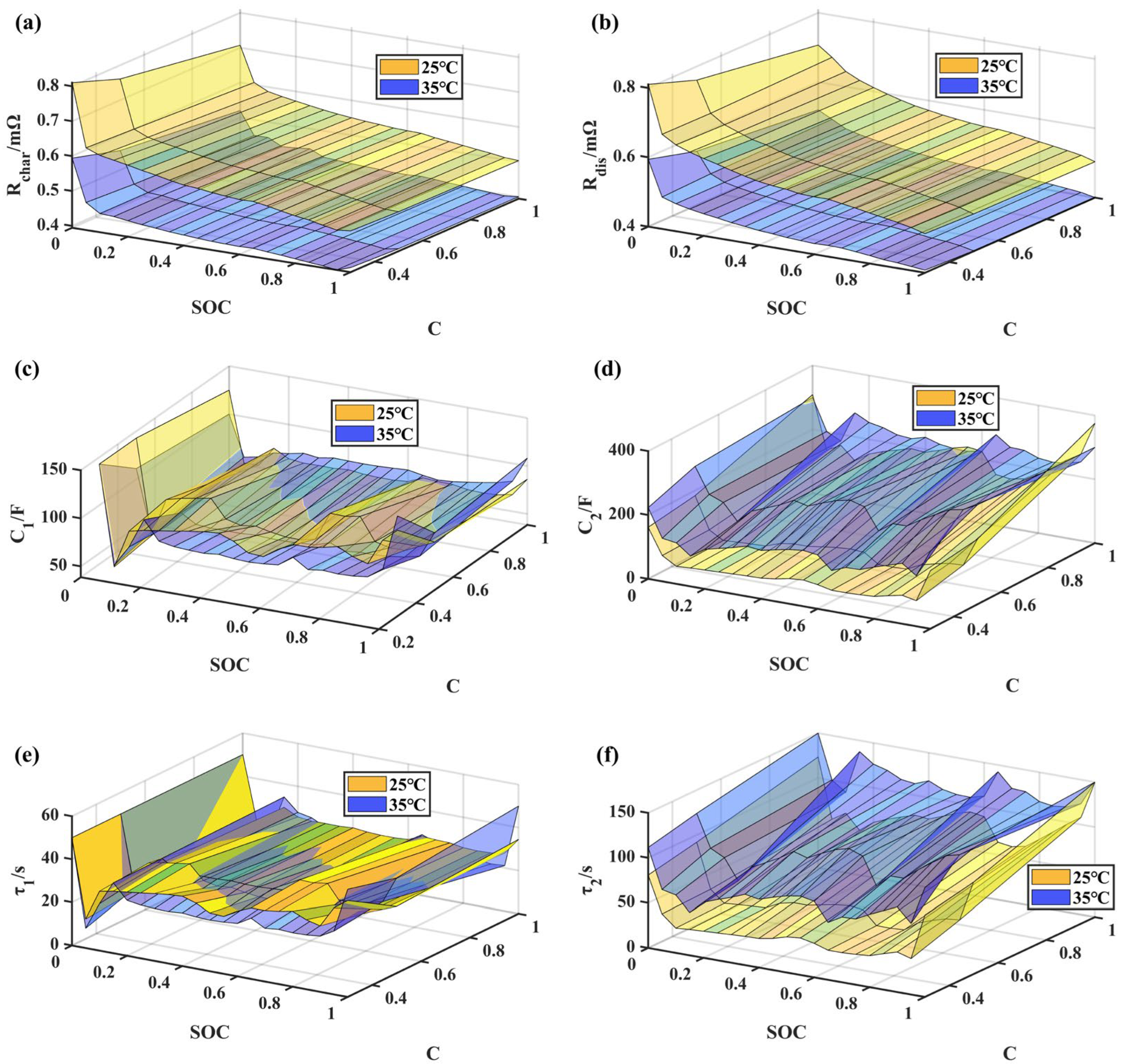
2. HPPC experiment① Charge at a CCCV of 1/3C at 25 °C, with a cut-off current of 6 A (1/20C).
② Perform SOC adjustment by discharging at 1/3C current and adjusting SOC by 0.05 at each step at temperatures of 25 °C and 35 °C.
The SOC adjustment path:
1 → 0.95 → 0.9… 0.1 → 0.05 → 0.
③ Perform current pulse excitation at each SOC experimental point at temperatures of 25 °C and 35 °C:
  • Discharge at 1/3C for 30 s, rest for 40 s, charge at 1/3C for 30 s, and rest for 10 min.
  • Discharge at 1/2C for 30 s, rest for 40 s, charge at 1/2C for 30 s, and rest for 10 min.
  • Discharge at 1C for 30 s, rest for 40 s, charge at 1C for 30 s, and rest for 10 min.
For SOC 1, only perform discharge pulses, and for SOC 0, only perform charge pulses.
Experimental results are shown in Figure 3a,b.
3.1. Main hysteresis experiment① Charge at a CCCV of 1/3C at 25 °C, with a cut-off current of 6 A (1/20C).
② Adjust SOC by discharging at a current of 1/3C at temperatures of 25 °C and 35 °C, with each adjustment being 0.05 SOC.
The SOC adjustment path is as follows:
1 → 0.95 → 0.9 →… → 0.1 → 0.05 → 0 → 0.05 → 0.1 → … → 0.95 → 1
③ At temperatures of 25 °C and 35 °C, allow the battery to rest for 3 h after reaching each SOC node and record the OCV value.
Experimental results are shown in Figure 3c.
3.2. Minor hysteresis experiment-I① Charge at a CCCV of 1/3C at 25 °C, with a cut-off current of 6 A (1/20C).
② Adjust SOC by discharging at a current of 1/3C at temperatures of 25 °C and 35 °C, with each adjustment being 0.05 SOC.
The SOC adjustment path is as follows:
1 → 0.95 → … → 0.15 → 0.2 → 0.25 → … → 0.75 → 0.8 → 0.75 → … → 0.15 → 0.2 → 0.25 → … → 0.95 → 1
③ At temperatures of 25 °C and 35 °C, allow the battery to rest for 3 h after reaching each SOC node.
Experimental results are shown in Figure 3d.
3.3. Minor hysteresis experiment-II① Charge at a CCCV of 1/3C at 25 °C, with a cut-off current of 6 A (1/20C).
② Adjust SOC by discharging at a current of 1/3C at temperatures of 25 °C and 35 °C, with each adjustment being 0.05 SOC.
The SOC adjustment path is as follows:
1 → 0.95 → … → 0.35 → 0.4 → 0.45 → … → 0.55 → 0.6 → 0.55 → … → 0.35 → 0.4 → 0.45 → … → 0.95 → 1
③ At temperatures of 25 °C and 35 °C, allow the battery to rest for 3 h after reaching each SOC node.
Experimental results are shown in Figure 3e.
4. Battery entropy heat experiment.① Charge at a CCCV of 1/3C at 25 °C, with a cut-off current of 6 A (1/20C).
② Discharge at a current of 1/3C at 25 °C to adjust SOC, with each adjustment being 0.1. The SOC adjustment path is as follows:
1 → 0.9 → … → 0.1 → 0
③ At each SOC node, adjust the temperature of the thermal chamber. The temperature adjustment path is as follows:
25 °C → 35 °C → 25 °C → 15 °C → 5 °C → −5 °C
Rest for 5 h at 5 °C and −5 °C, and rest for 3 h at other temperature points.
Calculate the derivative of OCV to temperature.
Experimental results are shown in Figure 3f.
5. Multi-rate CC core temperature acquisition experiment.① Charge at a CC of 1/3C, 1/2C, and 1C at 25 °C until the upper cut-off voltage of 3.65 V.
② Discharge at a CC of 1/3C, 1/2C, and 1C at 25 °C until the lower cut-off voltage of 2.5 V.
Experimental results are shown in the Section 2.3.2.
6. FR working condition experiment① Charge at a CCCV of 1/3C at 25 °C, with a cut-off current of 6 A (1/20C).
② Simulate operating conditions using the processed FR instructions at 25 °C.
The experimental results are shown in the Section 2.4.
Table 3. Thermal model parameters.
ItemSymbolSpecification
Heat conductivity coefficient (W/(m·K)) λ w 7.5
λ h 5
λ l 1.5
Convective heat transfer coefficient (W/(m2·K)) W 5
Specific heat capacity (J/(kg·K)) C i n 880
C s 880
Table 4. EKF algorithm.
ItemMathematical Expression
Initialize state variables
and covariance matrix
x 0 , P 0 , ω , v
Prior estimation x ^ t = A x ^ t 1 + + B u t 1 + ω t 1
Update covariance matrix P t = A P t 1 + A T + ω
Calculate Kalman gain K t = P t C T ( C P t C T + v ) 1
Posterior estimation x ^ t + = x ^ t + K t ( T s , m y t )
Update covariance matrix P t + = P t K t H P t
Table 5. RMSE of temperature simulation results.
Item1/3C1/2C1C
Internal temperature simulation RMSE (°C)0.220.390.75
Surface temperature simulation RMSE (°C)0.0070.0080.01
Disclaimer/Publisher’s Note: The statements, opinions and data contained in all publications are solely those of the individual author(s) and contributor(s) and not of MDPI and/or the editor(s). MDPI and/or the editor(s) disclaim responsibility for any injury to people or property resulting from any ideas, methods, instructions or products referred to in the content.

