1. Introduction
The use of fossil fuels on earth not only leads to an imbalance between energy supply and demand, but also increases the emission of harmful gases such as carbon dioxide and sulfur dioxide, causing environmental pollution problems [
1]. Humans are actively exploring how to replace them with renewable and sustainable energy sources. Wind energy has become a highly publicized alternative to nonrenewable energy sources [
2]. Furthermore, wind energy is receiving more and more attention because it is crucial for achieving carbon neutrality goals and transitioning to clean low-carbon energy [
3]. However, the variability and intermittency of wind speed can lead to various issues, including damage and voltage problems in wind power generation systems [
4]. Therefore, developing accurate wind speed prediction models is crucial for the energy sector. In past research, scholars have proposed various prediction models [
5], which can be classified into physical models, standard statistical models, and artificial intelligence-based models.
The physical models are mainly based on numeric weather prediction (NWP) and usually consider physical properties such as temperature, pressure and density [
6]. Pan et al. proposed a method for solving the probability prediction problem in the wind speed domain, which is a hybrid NWP combining current and future predicted numerical weather time series [
7]. Zhao et al.’s optimized NWP data are used to forecast wind speed for the coming day [
8]. Although the short-term prediction result of the NMP model is poor, it has strong long-term prediction ability [
9].
The statistical model makes full use of historical and future data to obtain forecasting results [
10], such as the autoregressive moving average (ARMA) [
11], autoregressive integrated moving average (ARIMA) [
12], and the Kalman filter (KF) [
13]. Lydia et al. proposed two types of the AR model to solve the ten-minute and one-hour ahead wing speed forecasting shortcoming [
14]. In North Dakota, a part of ARIMA was established to deal with one-day and two-day advance wind speed forecasting problems [
15]. Liu et al. proposed a seasonal ARIMA model to apply to the offshore wind speed forecasting [
16]. However, the wind speed time series has nonlinear characteristics, and statistical models are constrained by linear assumptions [
17], making it difficult to capture suitable forecasting models.
Artificial intelligence methods have been used to capture nonlinear features to overcome the limitations of statistical models [
18]. Many researchers have started to apply these methods for wind speed prediction. By using large amounts of historical data for training, AI methods can effectively adapt to the complex nonlinearity and uncertainty of wind speed time series [
19]. Artificial intelligence (AI) methods have become the dominant and superior wind speed prediction models and are classified into three types: single models, hybrid models, and integrated models.
Common AI methods include artificial neural networks (ANN) [
20], extreme learning machines (ELM) [
21], and the support vector machine (SVM) [
22]. With the development of neural networks, many neural networks with special structures have also been applied to wind speed prediction [
23], such as the adaptive wavelet neural network [
24], Emmanuel neural network (ENN) [
21], and long and short term memory network (LSTM) [
25]. Although a single model outperforms physical and statistical models, wind speed predictions from a single model are poor due to inherent drawbacks and the complex fluctuations in wind speed data, where linear and nonlinear features are always present in the data [
26].
The hybrid model can repair the defects of the single model and further improve the forecasting model by combining the single model with an optimization algorithm [
27]. Wang et al. proposed to tune the parameters in the support vector machine using the cuckoo search and genetic algorithm to improve the predictive performance of the model [
28]. Research data preprocessing techniques such as integrated empirical mode decomposition (EEMD) [
29], variational mode decomposition (VMD), and singular spectral analysis (SSA) [
30] apply them to wind speed forecasting to improve the forecasting results of the model. In [
31], an improved atomic search optimization algorithm (IASO) was used to search the extreme learning machine (ELM) to improve the wind speed prediction performance of the basic version. Fu et al. combined a Volterra series model with the VMD method to improve the beetle antenna search-based optimization algorithm and develop a new hybrid wind speed forecasting method [
32].
Due to the high correlation between hybrid models and the performance of a single model, it is difficult for hybrid models to handle different time series, while ensemble models have advantages in time series forecasting [
33]. Therefore, ensemble models have become the main method of wind speed forecasting. Wang et al. proposed an integration method consisting of an ANN, multi-objective bat algorithm (MOBA), and SSA to forecast wind speed [
34]. Altan et al. proposed optimizing LSTM networks for wind speed prediction based on the GWO algorithm, and the results showed that optimizing LSTM using the GWO algorithm can be very competitive [
35]. Wang et al. proposed an integrated model comprising CEEMD, ENN, and a multi-objective whale optimization algorithm (MOWOA) to predict short-term wind speeds [
36]. Liu et al. proposed a wind speed forecasting ensemble system based on a data decomposition method, optimal subsequence predictor, and ensemble technology through multi-objective optimization [
37]. Yang et al. adopted an integrated forecasting model based on decomposition technology and an optimization algorithm for integrating subsequence forecasting results, which has become an effective and promising method [
38].
Based on the above analysis, a new ensemble forecast model is developed in this paper in order to achieve higher forecast accuracy. Firstly, the best model is determined by the comparison of single models. Secondly, the original wind speed series are decomposed and reconstructed by using data preprocessing techniques, and the single model is optimized by using the egret population optimization algorithm to set the parameters in the appropriate threshold range and continuously update and iterate to achieve a more accurate optimization effect and then make wind speed forecasts.
The main contributions of this paper are as follows: Firstly, the number of decomposition layers in the variational modal decomposition technique is discussed, and the optimal parameter values are determined by comparing the model performance, so that the original wind speed time series can be decomposed, denoised, and reconstructed, effectively improving the forecast accuracy of the model. Secondly, the definition domain of the parameters of the egret population optimization algorithm is discussed, and the best definition domain is determined by setting different definition domains for forecasting; then, the support vector machine is optimized, and the optimized support vector machine is further used to forecast the wind speed time series. The prediction accuracy is improved; in addition, the proposed innovative integrated model is trained and tested based on wind speed data from several sites of a large wind farm, and the results show that the model outperforms the traditional model. Therefore, the model can be applied to wind speed prediction in wind power plants.
The research content of this article is as follows: the second section introduces the methods used in the model; the third section mainly introduces the test criterion; the fourth section introduces data processing and analysis; the fifth section discusses the number of layers of VMD, the definition domain of the egret population optimization algorithm, and the DM test; and the sixth section is a summary.
2. Methodology
The methodology mainly contains an advanced data decomposition method, new optimization algorithm, and the mentioned ensemble model.
2.1. Variational Mode Decomposition (VMD) Technique
During decomposition, VMD requires a minimum sum of the estimated bandwidths for each modality. It is constrained by the fact that the sum of the decomposed modes is equal to the original signal. Then, the corresponding constraint variational problem is represented as
where
represents the initial signal,
is all the modals,
k is the number of modal decomposition layers,
t is the time,
j is an imaginary number,
is the center frequency of the
kth component, and
δ(
t) is the Dirac distribution.
Lagrange multipliers are usually used to solve constrained problems. Therefore, in variational problems, the weights can be implemented using augmented Lagrange quantities to achieve better convergence and finiteness. Assuming no constrained problems, the VMD algorithm embeds quadratic penalties and Lagrange multipliers into the optimization process to ensure a constrained strictly conditional environment using the following extended expressions, which in turn transforms the optimization problem mentioned above into an unconstrained problem.
where
α represents the secondary penalty factor that reduces Gaussian noise interference, and
λ is the Lagrange multiplier. The variational problem described above is solved using the alternating direction multiplier method (ADMM), and the optimization of the unconstrained problem can be expressed as
where
represents the Wiener filter of
, and
indicates the center of gravity of the power spectrum of the mode function.
2.2. Support Vector Machine
Support vector machines are usually used for data regression prediction. When dealing with nonlinear problems, kernel functions can be introduced. To simplify the processing of nonlinear problems, low-dimensional problems can be transformed into high-dimensional linear problems, which are applicable to complex signal problems. Gaussian radial basis function is a kernel function with strong localization ability, which can map samples to high-dimensional space, with wide application, better performance, and less parameters compared with other kernel functions.
where
is the width of kernel function. The optimization problem is transformed into the following equation:
where
D is penalty factor. The most optimal nonlinear regression function can be obtained.
2.3. Egret Swarm Optimization Algorithm
The egret population optimization algorithm has development, exploration, comprehensive performance, stability, and convergence, in addition to the excellent performance and robustness of the ESOA algorithm in typical optimization applications [
39]. ESOA consists of three main components: The sit-and-wait strategy, the aggressive strategy, and the discrimination condition. Each egret group is composed of n egret teams, with each team consisting of three egrets. Egret A uses the waiting strategy, while Egret B and Egret C use the random walk and surrounding mechanism of the aggressive strategy, respectively.
- (1)
Sit and wait strategy:
The observation equation of the
,
is the true fitness obtained at each iteration, the pseudo-gradient
is the weight in the observation equation. The update location for egret A is as follows:
where
n is the current iteration number;
is the maximum number of iterations and hop is the range of feasible domains for arguments.
- (2)
Aggressive strategies: Egret B is a random walk, and then updated as follows:
is the random number between .
Egret C is an encirclement strategy, and the updated location is as follows:
where
and
are the optimal values for egret teams and egret populations, respectively;
and
are random numbers between (0, 1).
- (3)
Discrimination condition: After each egret in the egret squad calculates the updated position, it will jointly decide the update position of the egret squad, in the form below:
If , the egret squad chose to accept this option. Or if the random number r ∈ (0, 1) is less than 0.3, this means that there is a 30% chance of accepting a worse plan.
2.4. Data Feature Analysis Method
In most cases, developing a forecasting model involves computationally large complexity; so, in this article, we develop a suitable multiscale model to measure the complexity of the input data.
The Lempel–Ziv method measures the complexity characteristics of a time series. The smaller the Lempel–Ziv value of the sequence, the lower the complexity of the sequence, which means that the sequence contains more periodic components, stronger regularity, and less implicit frequency information. On the contrary, the larger the Lempel–Ziv value of the sequence, the higher the complexity, the worse the regularity of the feature, and the higher the frequency of the sequence. This article uses Lempel–Ziv algorithm to measure the complexity of the pattern, thereby improving the performance of the forecasting model.
To measure the complexity of Lempel–Ziv, it is necessary to convert the data series into a symbol sequence by comparing the data with a threshold, replacing a specific piece of data with 0 if the sequence is less than the threshold, otherwise replacing it with 1, and then analyzing the symbol sequence by identifying different quantities. When using the VMD method, applying the Lempel–Ziv method to identify the components, it is possible to select the optimal model for each component.
2.5. The Proposed Multiscale for Wind Power System
We propose a hybrid model framework, as shown in
Figure 1, which is mainly composed of data decomposition technology, single model prediction, and an intelligent optimization algorithm.
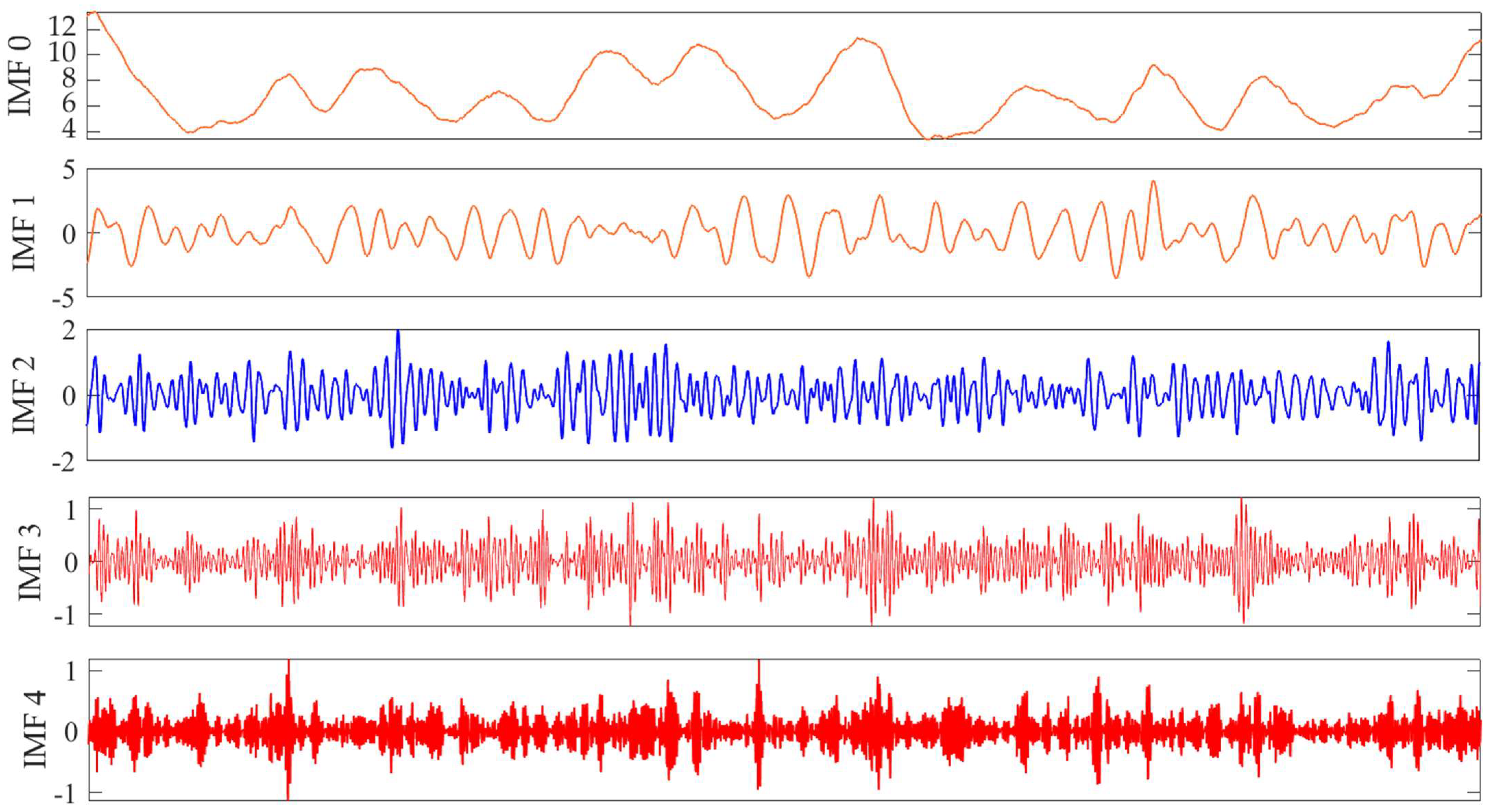
Stage 1: The original wind speed time series is decomposed using variational model decomposition technology to remove noise and random fluctuations, thus decomposing into a set of IMF. To distinguish these components, the Lempel–Ziv algorithm is used to calculate the complexity of these components, and each component is predicted based on the identified data features.
Stage 2: Forecasting of single models. For single model prediction, ELM, ENN, naïve, and SVM with high accuracy are used as single models for prediction in this study to build the developed combined model. Therefore, the results of single model prediction are shown in
Figure 1.
Stage 3: Determine the optimal weight coefficient for the forecasting model. Egret population optimization algorithm is used to continuously iteratively optimize the preprocessed data until the maximum number of iterations is reached, and the SVM of a single model is predicted according to the obtained model weight coefficient, so as to obtain the final prediction result.
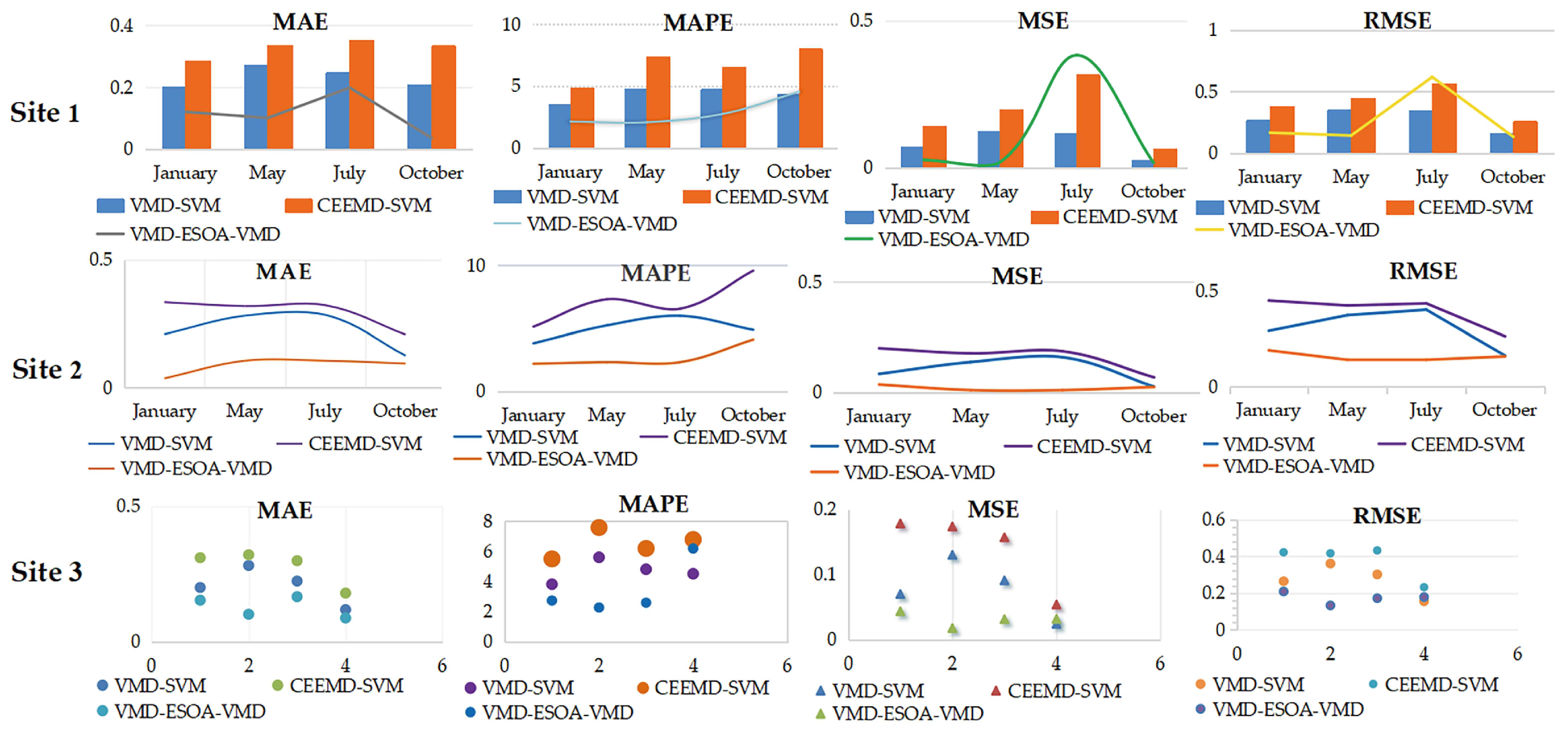
Stage 4: Considering the complex seasonality of wind speed, this study selected four quarters of data to verify that the established model can solve the problem of wind speed prediction in different seasons. By comparing the data from four quarters with different models, the superiority of the developed model compared to the comparative model is demonstrated from different perspectives.
6. Conclusions
As an important part of green renewable energy, wind energy is widely used to cope with environmental pollution and climate change. Therefore, high-precision and high-efficiency wind speed forecasting methods are essential to improve the operational efficiency of wind power generation systems. In this study, we successfully developed a new ensemble model based on data denoising techniques, the egret optimization algorithm, and a support vector machine. We also used the VMD method to decompose wind speed time series into components with different features to improve prediction accuracy and reduce noise interference. We compared our results with the CEEMD ensemble model based on multiscale hybrid prediction and single models.
The relevant conclusions of the proposed ensemble model are as follows: Firstly, the number of decomposition layers in the data decomposition technique was discussed to determine the optimal parameter values by comparing the model performance such as MAE, MAPE, MSE, and RMSE to decompose, denoise, and reconstruct the original wind speed time series, which effectively improved the forecast accuracy of the model. Secondly, the definition domains of the parameters of the egret population optimization algorithm were discussed, and the optimal definition domain was determined by setting different definition domains for forecasting, the support vector machine was optimized, and the optimized support vector machine was further used to forecast the wind speed time series. The accuracy of the developed model was further demonstrated by comparing the developed model with other models and by DM testing. Based on the various analyses in this study, the developed ensemble model effectively improves the accuracy of wind speed prediction and provides a more effective and accurate method for wind speed forecasting.
In the future, it is recommended to consider and construct common multiscale hybrid models using other univariate forecasting methods. To determine the usefulness of multiscale models in time prediction, the accuracy of the proposed model parameters and the sensitivity of the procedure should be considered when using data for forecasting. By discovering more single and mixed models and conducting diversified comparisons, useful insights can be provided on how to improve the predictive performance of multiscale models and offer valuable recommendations.


