Prediction of Gas Hydrate Formation in the Wellbore

Abstract

The formation of gas hydrates due to temperature and pressure changes during gas storage in the wellbore poses significant danger, necessitating the prediction of temperature and pressure distribution as well as of hydrate formation locations. We establish a temperature model that couples total thermal resistance and temperature in the wellbore-stratum composite medium system. Utilizing the two-phase pressure model alongside the temperature model, we conduct coupling calculations of temperature and pressure. Based on both temperature and pressure distribution within the wellbore and hydrate formation curve, we predict hydrate formation regions during production and analyze factors influencing temperature and pressure distribution. Results indicate that gas production rate and specific gravity of natural gas are major influencers on wellbore temperature and pressure distribution, while production time has minimal impact.

1. Introduction

Currently, many systems for gas storage are repurposed from former gas and oil reservoirs. However, these reservoirs may have undergone water flooding, leading to the formation of natural gas hydrates during the gas storage process. In addition, natural gas hydrate deposits can also occur during development [1,2,3]. Hydrates could cause blockage of pipes and freezing of gas nozzles, which would significantly affect the productivity of gas wells. Therefore, preventing the formation of hydrates in the wellbore is crucial for the safe and efficient production of gas wells. Hydrates are ice-like compounds of gas and water. The formation of natural gas hydrates is related to the local supersaturation of natural gas, which can be evaluated by the hydrate formation pressure (HFP) and hydrate formation temperature (HFT) under thermodynamically stable conditions [4]. At a given temperature, an increase in pressure above the HFP results in the production of gas hydrates. On the other hand, if the pressure remains constant, gas hydrates can form at temperatures below the HFT [5]. Thus, it is significant to accurately predict the temperature and pressure distribution in the wellbore.

Research on wellbore heat transmission has been carried out for many years. Ramey [6] was the first to divide the heat transfer process in the wellbore into three parts: single-phase fluid in the tube, the wellbore itself, and the surrounding formation. He developed a theoretical model for wellbore heat transfer that has since become one of the most widely used in the field. Hagoort [7] confirmed the accuracy of Ramey’s model, but observed that it produced large errors in predicting the overall heat transfer coefficient of the wellbore when Fourier time is short. As a result, it may not be suitable for accurately predicting temperature distribution in the wellbore during the early stages of production. Galvao et al. [8] developed a method that incorporates Joule–Thomson (J–T) effects, adiabatic fluid expansion, and fluid compressibility in the prediction of temperature-flow profiles, while their method only considered density as a function of temperature and ignored the impact of pressure. Most scholars rely on the overall heat transfer coefficient of the wellbore when calculating temperature distribution [9,10,11]. However, the determination of the coefficient involves numerous parameters that may not be suitable for rapid engineering predictions. Additionally, few studies have examined the impact of wellbore heat capacity on temperature distribution.

Models for predicting pressure drop in the wellbore primarily consist of empirical models [12,13,14,15] and theoretical models [16,17,18,19,20]. Gray [11] developed an empirical pressure drop model for condensate gas wells that includes four parameters. Woldesemayat and Ghajar [20] compared various void fraction models, including Lockhart and Martinelli [21], Coddington and Macian [12], Petalas and Aziz [22]. Their results indicated that the void fraction correlations based on the drift flux analysis method, such as Toshiba’s model [13] and Dix’s model [14], are more accurate. Hasan et al. [15] proposed a simplified two-phase flow model for the wellbore that avoided discontinuity issues at the transition of flow patterns by smoothing flow parameters near the flow pattern boundary. In addition, it is essential to consider the interaction between temperature and pressure of the fluid when predicting the pressure distribution in the wellbore [16,17,18,21].

The commonly used methods for hydrate prediction include the empirical equation method [23,24,25,26,27], K-value method [28], and thermodynamic method [29,30,31]. Hammerschmidt et al. [32] derived a correlation between hydrate melting point and pressure through experimental data fitting. However, the obtained correlation is based on a fixed gas composition and may have limited applicability. Ghiasi [19] developed functions for HFT based on gas pressure and molecular weight, providing different equations for various molecular weights. In addition, Motiee [23] and Ghayyem, et al. [24] also proposed empirical formulas to predict hydrate formation conditions in different scenarios. The K-value method, which belongs to the phase equilibrium theory, involves determining a gas-solid equilibrium constant by consulting a constant equilibrium chart. However, the K-value method is limited to a specific range of pressure, up to 13.8 MPa for methane, ethane, and propane, up to 6.9 MPa for carbon dioxide and up to 13.8 MPa for hydrogen sulfide and nitrogen [25,33]. Beyond this range, it tends to yield higher results than that of the empirical equations method. Van der Waals and Plateeuw [26] proposed a statistical thermodynamic model for hydrate formation based on its thermodynamic mechanism, in which they treated the hydrate as an ideal solid solution. Later, Ballard et al. [27,28,29] conducted multiple studies by utilizing thermodynamic methods to predict hydrate formation.

Despite the existence of various temperature, pressure drop, and hydrate prediction models for the wellbore, there remains a lack of systematic research on temperature distribution, pressure distribution, and hydrate formation. Therefore, the aim of this work is to undertake a comprehensive study of the impact of various factors on the temperature distribution, pressure distribution, and location of hydrate formation in the wellbore. Section 2 introduces the temperature models, pressure drop models of the wellbore, and hydrate prediction models. Subsequently, Section 3 discusses the factors that influence the temperature distribution, pressure distribution, and hydrate formation in the wellbore. Finally, Section 4 presents the conclusions drawn from this work.

2. Theories and Models

2.1. Temperature Distribution Models

During the production process, natural gas flows from underground through the wellbore, resulting in heat transfer due to temperature differences between the fluid and formation. Assuming a one-dimensional stable flow for the fluid in the wellbore, the energy balance for a control volume of unit length within the wellbore (as shown in Figure 1) is obtained [32]:

$$q_{\mathrm{l}}=\frac{\mathrm{d}(mE{)}_{cv}}{\Delta z \mathrm{d}t}+\frac{\mathrm{d}(mE{)}_w}{\Delta z \mathrm{d}t}+\frac{\mathrm{d}}{\mathrm{d}z}\left[G_{\mathrm{m}}(h+0.5v^2+gz)\right]$$

(1)

where q_l is the heat exchange amount between the fluid and formation per unit length of the wellbore, W/m. E is the internal energy of the fluid, J/kg. m is the mass of the fluid in the control volume, kg. h is the enthalpy of the fluid, J/kg. G_m is the mass flow of fluid, kg/s. v is the flow velocity of the fluid, m/s. g is the gravity, m/s², z is the height of the wellbore, and the subscripts cv and w denote the control volume and wall, respectively.

By disregarding the heat transfer in the axial direction, we can introduce a heat transfer coefficient per unit length of the wellbore denoted by k_l. This leads to the expression of q_l as follows:

$$q_{\mathrm{l}}=k_{\mathrm{l}}(T_{\mathrm{e}}-T_{\mathrm{f}})$$

(2)

where k_l is the heat transfer coefficient per unit length of the wellbore. This value is the reciprocal of the total thermal resistance, W/(m·K); T_e is the temperature of formation, and K; T_f is the temperature of the fluid, K.

The enthalpy of natural gas conforms to the fundamental equation of thermodynamics, given as follows:

$$\frac{\mathrm{d}h}{\mathrm{d}z}=C_{\mathrm{p}}\frac{\mathrm{d}T}{\mathrm{d}z}+{(\frac{\partial h}{\partial p})}_{\mathrm{T}}\frac{\mathrm{d}p}{\mathrm{d}z}=C_{\mathrm{p}}\frac{\mathrm{d}T}{\mathrm{d}z}-C_{\mathrm{p}}{\alpha }_{\mathrm{H}}\frac{\mathrm{d}p}{\mathrm{d}z}$$

(3)

where C_p is the heat capacity of the fluid, kJ/(kg·K); p is the pressure of the fluid, and MPa; α_H is the Joule-Tomson coefficient, K/MPa.

Based on the above formulas, we can derive the expression for the temperature gradient along the vertical direction within the wellbore as follows:

$$\frac{\mathrm{d}T}{\mathrm{d}z}=\frac{k_{\mathrm{l}}}{G_{\mathrm{m}}{C}_{\mathrm{p}}}(T_{\mathrm{e}}-T_{\mathrm{f}})+{\alpha }_{\mathrm{H}}\frac{\mathrm{d}p}{\mathrm{d}z}-\frac{g}{C_{\mathrm{p}}}$$

(4)

In the present work, k_l is used to measure the heat transfer capacity of the wellbore. Then, the thermal resistance of the wellbore, as shown in Figure 2, is given as follows:

$$\begin{array}{l}{k}_{\mathrm{l}}=\frac{1}{R_{\mathrm{total}}}=\frac{1}{R_{\mathrm{f}} + R_{\mathrm{tub}} + R_{\mathrm{ann}} + R_{\mathrm{cas}} + R_{\mathrm{cem}} + R_{\mathrm{earth}}}=\\ \frac{1}{\frac{1}{2\pi r_{\mathrm{ti}}{h}_{\mathrm{f}}}+\frac{1}{2\pi {\lambda }_{\mathrm{tub}}}\ln \frac{r_{\mathrm{to}}}{r_{\mathrm{ti}}}+\frac{1}{2\pi {\lambda }_{\mathrm{E}}}\ln \frac{r_{\mathrm{ci}}}{r_{\mathrm{to}}}+\frac{1}{2\pi {\lambda }_{\mathrm{cas}}}\ln \frac{r_{\mathrm{co}}}{r_{\mathrm{ci}}}+\frac{1}{2\pi {\lambda }_{\mathrm{cem}}}\ln \frac{r_{\mathrm{h}}}{r_{\mathrm{co}}}+\frac{1}{2\pi {\lambda }_{\mathrm{earth}}}f(\mathrm{t})}\end{array}$$

(5)

where R_f, R_tub, R_ann, R_cas, R_cem, R_earth represent the convective thermal resistance between tubing and fluid, the thermal resistance of tubing, the thermal resistance of annular fluid, the thermal resistance of casing, the thermal resistance of cement loop, and the thermal resistance of formation, respectively, (m·K)/W.

Based on the results of Cheng et al. [30], we consider the transient heat-conduction time function, f(t), as a function of wellbore heat capacity, formation heat capacity, and dimensionless time. Then the heat–conduction time function f(t) can be given as

$$f(t)=\ln (2\sqrt{{\tau }_{\mathrm{D}}})-\frac{C_1}{2}+\frac{1}{4{\tau }_{\mathrm{D}}}\left[1+(1-\frac{1}{\omega })\ln (4{\tau }_{\mathrm{D}})+C_1\right]$$

(6)

where τ_D is dimensionless time; C₁ is the Euler’s constant, with the value of 0.5772; and ω is a dimensionless parameter representing the ratio of the formation heat capacity and the wellbore heat capacity.

2.2. Pressure Distribution Models

The continuity equation in the control volume can be obtained from the mass balance as follows:

$$\frac{\mathrm{d}(\rho vA)}{\mathrm{d}z}=0$$

(7)

where ρ is the density, kg/m³; v is the velocity, and m/s; A is the cross-sectional area of tubing, m².

The external force exerted on the fluid equals the momentum change of the fluid in a given control volume and can be calculated as:

$${\displaystyle \sum _{}^{}{F}_{\mathrm{z}}=\rho A\mathrm{d}z\frac{\mathrm{d}v}{\mathrm{d}\tau }}$$

(8)

The external force exerted on the fluid in a given control volume includes the gravity of fluid in the vertical direction ρgAdzsinθ, the differential pressure between inlet and outlet of control volume pA − (p + dp)A, and friction between the fluid and tubing τ_wπDdz, where τ_w is the friction per unit tubing area, Pa.

$${\tau }_{\mathrm{w}}=\frac{f}{4}\frac{\rho v^2}{2}$$

(9)

The equation of mass conservation of fluid in the wellbore during production could be obtained as follows:

$$-\frac{\mathrm{d}p}{\mathrm{d}z}=\rho g\sin \theta +f\frac{\rho v^2}{2D}+\rho v\frac{\mathrm{d}v}{\mathrm{d}z}$$

(10)

where θ is the inclination angle of the wellbore, and f is the frictional coefficient.

As can be seen from Equation (9), the pressure drop along the wellbore includes the gravity head, the friction head, and the dynamic head. The pressure drop per unit control volume length can be obtained by simply calculating the f and dv/dz. According to the recommendations in ref. [31], the frictional coefficient of mixed fluids could be calculated by Chen’s correlation:

$$f_{\mathrm{m}}={\left[4\log (\frac{\Delta /D}{3.7065}-\frac{5.0452}{{\mathrm{Re}}_{\mathrm{m}}}\log \Lambda )\right]}^{-2}$$

(11)

where Δ is the roughness of tubing, mm; Re_m is Reynolds number; D denotes the radius of tubing, mm; and Λ is a dimensionless number and can be calculated by the following formula:

$$\Lambda =\frac{(\Delta /D{)}^{1.1098}}{2.8257}+(\frac{7.149}{{\mathrm{Re}}_{\mathrm{m}}}{)}^{0.8981}$$

(12)

The dynamic head can be calculated by the following formula:

$$\frac{\mathrm{d}v}{\mathrm{d}z}=\frac{\mathrm{d}\left(G{A}^{-1}{\rho }^{-1}\right)}{\mathrm{d}z}=-\frac{G}{A{\rho }^2}\frac{\mathrm{d}\rho }{\mathrm{d}z}$$

(13)

2.3. Gas Hydrate Formation Models

Cao et al. [34] conducted a comparative study of the K-value method and the empirical equation method for predicting hydrate formation. The results indicated that the Ponomalev empirical formula method performs with greater accuracy, as derived from the regression of numerous experimental data. The Ponomalev formula for hydrate formation at varying specific gravities is given as follows:

$$\mathrm{When} T > 273.15 \mathrm{K}, \lg p=-1.0055+0.0541(B+T-273.1)$$

(14)

$$\mathrm{When} T\le 273.15 \mathrm{K}, \lg p=-1.0055+0.0171(B_1+T-273.1)$$

(15)

where parameters B and B₁ that relate to the specific gravity of natural gas are listed in

Table 1. The value of B and B₁ under different specific gravity.

Specific Gravity	0.56	0.60	0.64	0.66	0.68	0.70	0.75	0.80	0.85	0.90	0.95	1.0
B	24.25	17.67	15.47	14.76	14.34	14.00	13.32	12.47	12.18	11.66	11.17	10.77
B1	77.4	64.2	48.6	46.9	45.6	44.4	42.0	39.9	37.9	36.2	34.5	33.1

.

The formation pressure of hydrate at different temperatures can be obtained from the Ponomalev formula. When the temperature of the fluid is lower than the HFT at a certain pressure or the pressure of the fluid is greater than the HFP at a certain temperature, hydrate formation occurs at that specific depth of the wellbore. By following this principle, we can predict the location of hydrate formation within the wellbore.

In this study, the physical parameters of the fluid, such as density and specific heat capacity, are considered as temperature- and pressure-dependent functions, which have been derived from the REFPROP database [35]. The operation parameters of gas storage are shown in

Table 2. Operation parameters of gas storage.

Parameter	Value	Parameter	Value
Well depth/m	1800.0	Producing time/day	10.0
The inner diameter of tubing/mm	72.0	Water production rate t/d	12.69
The outer diameter of tubing/mm	114.0	Gas production rate m³/d	7292
The inner diameter of casing/mm	159.0	Pressure of bottom-hole/MPa	18.779
The outer diameter of casing/mm	177.8	Temperature of bottom-hole/°C	75.0
The outer diameter of cement/mm	245.0	Mean annual ground temperature/°C	12.0

.

3. Results and Discussion

3.1. Prediction of Hydrate Formation Region

Figure 3 shows the temperature and pressure distribution of the fluid in the wellbore and the HFP of a fixed component natural gas. As depicted in Figure 3a, hydrate formation requires a low-temperature and high-pressure environment, which is situated to the left of the HFP line (solid blue line). By determining the point of intersection between the two curves, we can estimate that hydrates will form at a fluid temperature of around 20 °C within the wellbore. The calculated and measured temperature and pressure along the wellbore are presented in Figure 3b. The temperature distribution is well predicted while the pressure is underpredicted at the near-ground position. This might be due to the fact that the input parameters in Table 2 are based on operational experience rather than experimental measurements, resulting in discrepancies between calculated and measured values. Furthermore, Figure 3b indicates that the depth range of 50~100 m will be subject to hydrate formation. It is worth noting that the HFP exponentially increases with temperature, suggesting that preventing hydrate formation is feasible if the temperature of the fluid at the wellhead remains above a specific value.

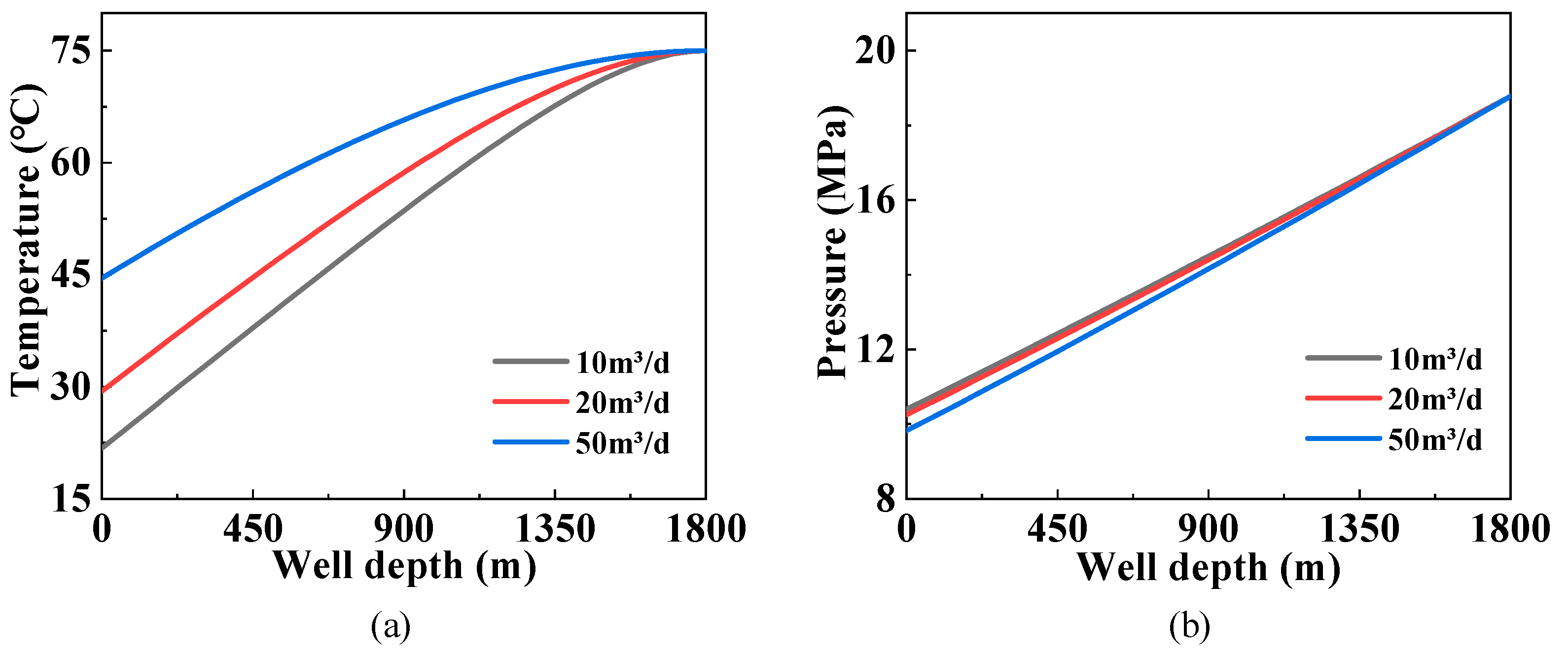
3.2. Influence of the Gas Production Rate

The gas production rate is a critical parameter that affects both the flow process and heat transfer. Therefore, this subchapter aims to explore how it influences the distribution of temperature and pressure. Figure 4a illustrates the temperature distribution of fluid under varying gas production rates. The plot highlights that the temperature change at the bottom of the well is relatively slow compared to other locations. This is attributed to the small temperature gap between natural gas at the bottom of the well and the formation, causing a sluggish rate of heat transfer. Additionally, when the gas production rate escalates, higher amounts of heat are transferred from the gas storage to the fluid per unit time, resulting in elevated wellbore fluid temperatures.

In Figure 4b, the wellhead pressure (WHP) of fluid is depicted under varying gas production rates. It can be observed that, for low gas production rates, the WHP increases as the gas production rate increases, whereas for high gas production rates, the WHP decreases with increasing gas production rate. This phenomenon can be explained by considering the total pressure drop, which is significantly influenced by gravity at low gas production rates. Specifically, an increase in gas production rate reduces the density of the mixed fluid, resulting in a smaller gravity head and higher fluid pressure (refer to Figure 4c). In contrast, when gas production rates are high, the total pressure drop is primarily governed by friction head. As the gas production rate increases, it leads to heightened fluid friction, thereby elevating the friction head and reducing the fluid pressure (see Figure 4d).

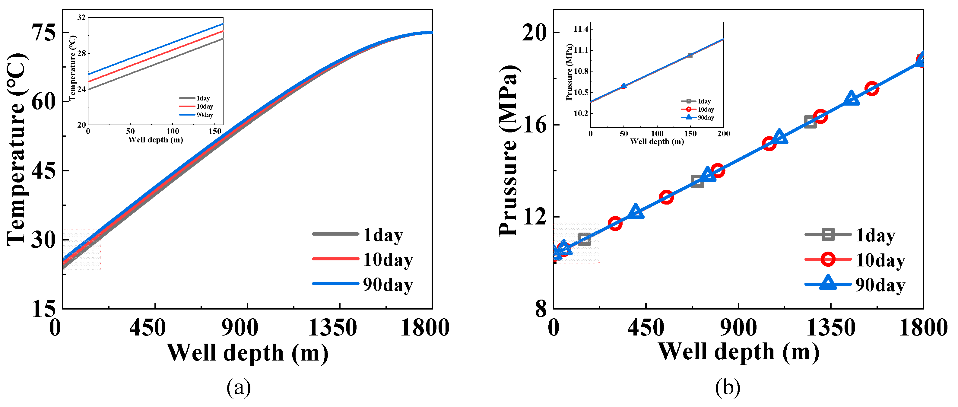
3.3. Influence of the Producing Time

Figure 5a,b illustrate the temperature and pressure distribution of fluid at varying production times, respectively. As indicated in Figure 5a, the fluid temperature slightly increases with longer production times due to ample heat exchange between the fluid and formation. In contrast, it is evident from Figure 5b that the fluid pressure is hardly impacted by production time, and the pressure distribution remains mostly uniform irrespective of the production time. This can be attributed to the rapid attainment of a stable state for fluid pressure.

3.4. Influence of the Water Production Rate

Figure 6a,b depict the temperature and pressure distribution of fluid at varying water production rates, respectively. It is evident from both figures that as the water production rate increases, the fluid pressure decreases while the fluid temperature increases. This phenomenon can be attributed to the fact that higher water production rates enable more heat transfer from the bottom of the well, causing a rise in fluid temperature. Moreover, an increase in water production rate leads to elevated mixed fluid density and gravity head, resulting in greater energy consumption of the mixed fluid from the bottom hole to the wellhead. Consequently, the fluid pressure along the wellbore decreases.

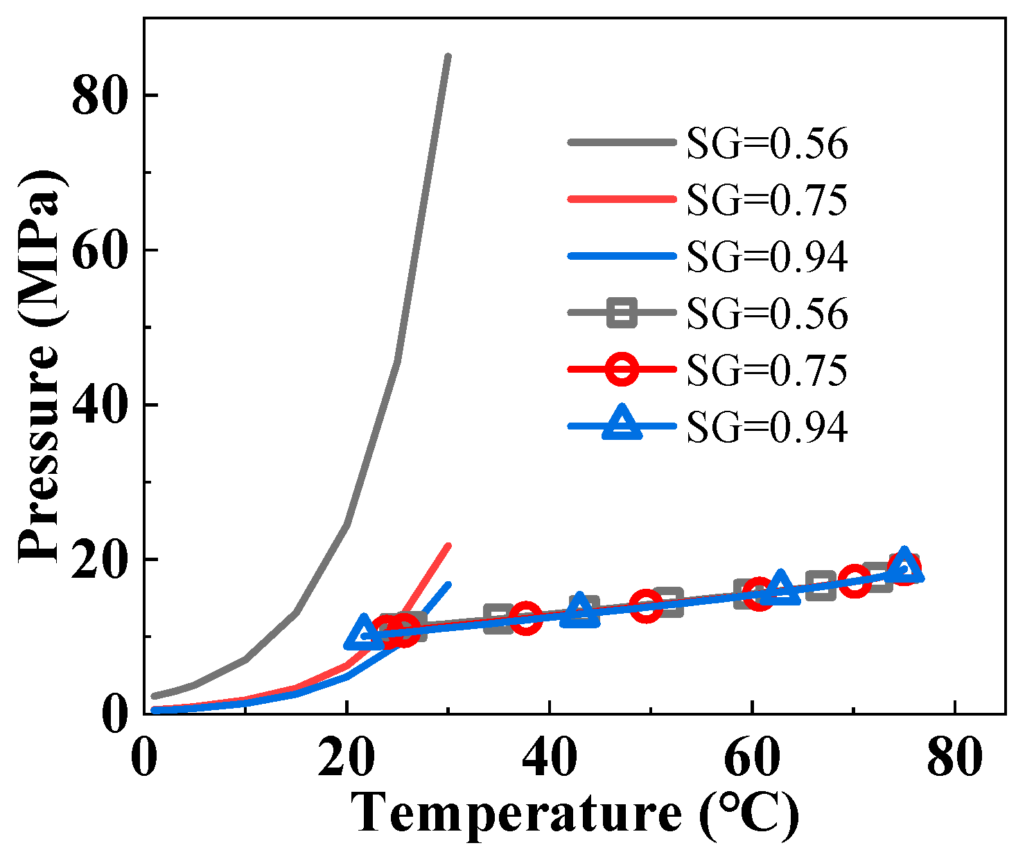
3.5. Influence of Natural Gas Components on Hydrate Formation

The impact of natural gas composition on hydrate formation within the wellbore is investigated in this section, assuming that natural gas is a mixture of methane and ethane. Three types of natural gas are employed with specific gravities of 0.56, 0.75, and 0.94, and corresponding methane mole fractions of 0.99, 0.6, and 0.2, respectively. Figure 7 illustrates the temperature and pressure distribution of fluid in the wellbore and HFP under different specific gravity values for natural gas. The solid lines represent the HFP for varying specific gravities, while the lines with symbols show the temperature and pressure values of the wellbore. The findings reveal that, with increasing specific gravity, both the HFP and temperature and pressure along the wellbore decrease, indicating easier hydrate formation during production. In other words, lower methane mole fractions facilitate hydrate formation. Table 1 further demonstrates that an increase in natural gas specific gravity corresponds to higher parameters B and B₁ and a lower HFP.

Further research could focus on refining the temperature model by incorporating additional parameters or factors that might affect temperature distribution in the wellbore and surrounding stratum. Additionally, investigating the impact of other variables, such as the composition of the gas or the presence of inhibitors, on hydrate formation and its relation to temperature and pressure distribution could provide valuable insights. Exploring the applicability of the findings in different geological conditions or wellbore designs would also contribute to a more comprehensive understanding of gas hydrate formation and its implications for gas storage production.

4. Conclusions

In this study, a wellbore temperature and pressure coupling model is established, and the wellbore temperature and pressure distribution of a gas well are calculated. The influence of the gas production rate, water production rate, and production time on the wellbore temperature and pressure distribution are analyzed. The results indicate that as gas production increases, the temperature of the wellbore fluid rises while the pressure of the wellhead fluid initially rises and then declines. Similarly, with an increase in water production, the temperature of the wellbore fluid increases while the extracted pressure decreases. As production time is prolonged, there is a slight rise in the temperature of the extracted well fluid, while the pressure experiences minimal changes. The gas production rate has the greatest impact, followed by the water production rate, while production time has minimal influence. The hydrate formation position in the wellbore is predicted by utilizing the Ponomalev empirical formula and considering the temperature and pressure distribution of fluid in the wellbore. The formation of gas hydrates is significantly influenced by the specific gravity of natural gas, with higher specific gravities leading to easier formation.

References

1. Klymenko, V.; Ovetskyi, S.; Martynenko, V.; Vytyaz, O.; Uhrynovskyi, A. An alternative method of methane production from deposits of subaquatic gas hydrates. Min. Miner. Depos. 2022, 16, 11–17. [Google Scholar] [CrossRef]
2. Bazaluk, O.; Sai, K.; Lozynskyi, V.; Petlovanyi, M.; Saik, P. Research into Dissociation Zones of Gas Hydrate Deposits with a Heterogeneous Structure in the Black Sea. Energies 2021, 14, 1345. [Google Scholar] [CrossRef]
3. Pedchenko, M.; Pedchenko, L.; Nesterenko, T.; Dyczko, A. Technological Solutions for the Realization of NGH-Technology for Gas Transportation and Storage in Gas Hydrate Form. Solid State Phenom. 2018, 277, 123–136. [Google Scholar] [CrossRef]
4. Botrel, T. Hydrates Prevention and Removal in Ultra-Deepwater Drilling Systems. In Proceedings of the Offshore Technology Conference, OTC, Houston, TX, USA, 30 April–3 May 2001; p. OTC-12962-MS. [Google Scholar]
5. Sahari Moghaddam, F.; Hamid, A.; Abdi, M.; James, L. Consideration of Various Parameters and Scenarios in the Simulation of Hydrate Formation. In Proceedings of the SPE Canadian Energy Technology Conference, SPE, Calgary, AB, Canada, 16–17 March 2022; p. SPE-208881-MS. [Google Scholar]
6. Ramey, H.J. Wellbore Heat Transmission. J. Pet. Technol. 1962, 14, 427–435. [Google Scholar] [CrossRef]
7. Hagoort, J. Ramey’s Wellbore Heat Transmission Revisited. SPE J. 2004, 9, 465–474. [Google Scholar] [CrossRef]
8. Galvao, M.S.; Carvalho, M.S.; Barreto, A.B. A Coupled Transient Wellbore/Reservoir-Temperature Analytical Model. SPE J. 2019, 24, 2335–2361. [Google Scholar] [CrossRef]
9. Willhite, G.P. Over-all Heat Transfer Coefficients in Steam And Hot Water Injection Wells. J. Pet. Technol. 1967, 19, 607–615. [Google Scholar] [CrossRef]
10. You, J.; Rahnema, H.; McMillan, M.D. Numerical modeling of unsteady-state wellbore heat transmission. J. Nat. Gas Sci. Eng. 2016, 34, 1062–1076. [Google Scholar] [CrossRef]
11. Gray, H.E. Vertical Flow Correlation in Gas Wells. User’s Manual for API 14B Surface Controlled Subsurface Safety Valve Sizing Computer Program, 2nd ed.; American Petroleum Institute: Washington, DC, USA, 1978. [Google Scholar]
12. Coddington, P.; Macian, R. A study of the performance of void fraction correlations used in the context of drift-flux two-phase flow models. Nucl. Eng. Des. 2002, 215, 199–216. [Google Scholar] [CrossRef]
13. Inoue, A.; Kurosu, T.; Yagi, M.; Morooka, S.; Hoshide, A.; Ishizuka, T.; Yoshimura, K. In-bundle void measurement of a BWR fuel assembly by an x-ray CT scanner: Assessment of BWR design void correlation and development of new void correlation. In Proceedings of the 2nd ASME-JSME International Conference on Nuclear Engineering, Chiba, Japan, 1 January 1993. [Google Scholar]
14. Morooka, S.; Ishizuka, T.; Iizuka, M.; Yoshimura, K. Experimental study on void fraction in a simulated BWR fuel assembly (evaluation of cross-sectional averaged void fraction). Nucl. Eng. Des. 1989, 114, 91–98. [Google Scholar] [CrossRef]
15. Hasan, A.R.; Kabir, C.S.; Sayarpour, M. Simplified two-phase flow modeling in wellbores. J. Pet. Sci. Eng. 2010, 72, 42–49. [Google Scholar] [CrossRef]
16. Duru, O.O.; Horne, R.N. Modeling Reservoir Temperature Transients and Reservoir-Parameter Estimation Constrained to the Model. SPE Reserv. Eval. Eng. 2010, 13, 873–883. [Google Scholar] [CrossRef] [Green Version]
17. Duru, O.O.; Horne, R.N. Simultaneous Interpretation of Pressure, Temperature, and Flow-Rate Data Using Bayesian Inversion Methods. SPE Reserv. Eval. Eng. 2011, 14, 225–238. [Google Scholar] [CrossRef]
18. Hasan, A.R.; Kabir, C.S.; Wang, X. Wellbore Two-Phase Flow and Heat Transfer During Transient Testing. SPE J. 1998, 3, 174–180. [Google Scholar] [CrossRef]
19. Ghiasi, M.M. Initial estimation of hydrate formation temperature of sweet natural gases based on new empirical correlation. J. Nat. Gas Chem. 2012, 21, 508–512. [Google Scholar] [CrossRef]
20. Woldesemayat, M.A.; Ghajar, A.J. Comparison of void fraction correlations for different flow patterns in horizontal and upward inclined pipes. Int. J. Multiph. Flow 2007, 33, 347–370. [Google Scholar] [CrossRef]
21. Lockhart, R.W. Proposed Correlation of Data for Isothermal Two-Phase, Two-Component Flow in Pipes. Chem. Eng. Prog. 1949, 45, 39–48. [Google Scholar]
22. Petalas, N.; Aziz, K. A Mechanistic Model for Multiphase Flow in Pipes. J. Can. Pet. Technol. 2000, 39, PETSOC-00-06-04. [Google Scholar] [CrossRef]
23. Motiee, M. Estimate possibility of hydrates. Hydrocarb. Process. 1991, 70, 98–99. [Google Scholar]
24. ali Ghayyem, M.; Izadmehr, M.; Tavakoli, R. Developing a simple and accurate correlation for initial estimation of hydrate formation temperature of sweet natural gases using an eclectic approach. J. Nat. Gas Sci. Eng. 2014, 21, 184–192. [Google Scholar] [CrossRef]
25. Wilcox, W.I.; Carson, D.B.; Katz, D.L. Natural Gas Hydrates. Ind. Eng. Chem. 1941, 33, 662–665. [Google Scholar] [CrossRef]
26. Van der Waals, J.H.; Platteeuw, J.C. Clathrate Solutions; John Wiley & Sons, Inc.: Hoboken, NJ, USA, 2007; pp. 1–57. [Google Scholar] [CrossRef]
27. Ballard, A.L.; Sloan, E.D. The next generation of hydrate prediction: Part III. Gibbs energy minimization formalism. Fluid Phase Equilib. 2004, 218, 15–31. [Google Scholar] [CrossRef]
28. Ballard, A.L.; Sloan, E.D., Jr. The next generation of hydrate prediction: I. Hydrate standard states and incorporation of spectroscopy. Fluid Phase Equilib. 2002, 194–197, 371–383. [Google Scholar] [CrossRef]
29. Jager, M.D.; Ballard, A.L.; Sloan, E.D. The next generation of hydrate prediction: II. Dedicated aqueous phase fugacity model for hydrate prediction. Fluid Phase Equilib. 2003, 211, 85–107. [Google Scholar] [CrossRef]
30. Cheng, W.-L.; Huang, Y.-H.; Lu, D.-T.; Yin, H.-R. A novel analytical transient heat-conduction time function for heat transfer in steam injection wells considering the wellbore heat capacity. Energy 2011, 36, 4080–4088. [Google Scholar] [CrossRef]
31. Chen, N.H. An Explicit Equation for Friction Factor in Pipe. Ind. Eng. Chem. Fundam. 1979, 18, 296–297. [Google Scholar] [CrossRef]
32. Hammerschmidt, E.G. Formation of Gas Hydrates in Natural Gas Transmission Lines. Ind. Eng. Chem. 1934, 26, 851–855. [Google Scholar] [CrossRef]
33. Carson, D.B.; Katz, D.L. Natural Gas Hydrates. Trans. AIME 1942, 146, 150–158. [Google Scholar] [CrossRef]
34. Cao, F.; Wang, T.; Cao, L.; Wang, B. Formation Conditions of Forecasting Natural Gas Hydrate with Numerical Calculation Method. Guangzhou Chem. Ind. 2013, 5, 82–83. [Google Scholar]
35. Lemmon, E.W.; Huber, M.; Mclinden, M.O. NIST Standard Reference Database 23: Reference Fluid Thermodynamic and Transport Properties—REFPROP, Version 9.1; Standard Reference Data Program; NIST: Gaithersburg, MD, USA, 2010. [Google Scholar]
Figure 1. Energy balance in control volume.
Energies 16 05579 g001
Figure 2. Thermal resistance of wellbore.
Energies 16 05579 g002
Figure 3. Prediction of the hydrate formation region: (a) HFP and the pressure of fluid vs. the temperature of fluid; (b) temperature and pressure distribution along the wellbore.
Energies 16 05579 g003
Figure 4. Influence of gas production rate: (a) temperature distribution; (b) well head pressure (WHP); (c) pressure distribution at low gas production rate; (d) pressure distribution at high gas production rate.
Energies 16 05579 g004
Figure 5. Influence of producing time: (a) temperature distribution; (b) pressure distribution.
Energies 16 05579 g005
Figure 6. Influence of water production rate: (a) temperature distribution; (b) pressure distribution.
Energies 16 05579 g006
Figure 7. Prediction of hydrate formation position under different specific gravity.
Energies 16 05579 g007