Abstract
As the penetration of renewable energy sources into a power system increases, the significance of precise short-term forecasts for wind power generation becomes paramount. However, the erratic and non-periodic nature of wind poses challenges in accurately predicting the output. This paper presents a comprehensive investigation into forecasting wind power generation for the following day, using three machine learning models: long short-term memory (LSTM), convolutional neural network-bidirectional LSTM (CNN-biLSTM), and light gradient boosting machine (LGBM). In addition, this paper proposes a method to improve the prediction performance of LGBM by separating data according to the distribution of features, and training and testing each separated dataset with a distinct model. This study includes a comparative analysis of the performance of the proposed models in predicting wind turbine output, offering valuable insights into their respective efficiencies. The results of this investigation were analyzed for two geographically distinct wind farms (Korea and the UK). The findings of this study are expected to facilitate the selection of efficient prediction models within the forecast accuracy auxiliary service market and assist grid operators in ensuring reliable power supply for the grid.
1. Introduction
In line with global efforts to combat environmental degradation and the growing trend of renewable energy adoption, the proportion of renewable energy sources in power systems is steadily increasing. Many countries worldwide are implementing legislation to accelerate renewable energy supply due to concerns over energy security resulting from unstable supply and demand. In a report titled ‘Renewable Energy Market’ released by the International Energy Agency (IEA) on 23 June, it was projected that the capacity of renewable energy generators globally will increase by about 107 GW, the largest growth ever recorded, reaching over 440 GW by 2023 [1]. The IEA argues that this growth is part of a broader effort to rapidly achieve energy security, as investments in clean energy facilities show signs of recovery following the subsidence of the COVID-19 pandemic [2]. As an example, in February 2023, the UK established a new “Energy Security and Net Zero” department, accelerating the transition from fossil fuels to renewable energy sources such as wind and solar. Following this, the UK unveiled ‘Powering up Britain’ and set a firm goal of achieving net zero by 2050 [3]. The EU announced REPowerEU in 2022 and set a target of 45% renewable energy by 2030 [4]. This target represents a 5% upward adjustment from the European Union’s carbon reduction legislative proposal ‘Fit-for-55’ [5] announced in 2021, compared to the initial target of 40%. In order to achieve this goal, the plan is to increase solar capacity by approximately 600 GW and wind capacity by approximately 510 GW by 2030. In the case of Korea, as of June 2023, according to the power generation facility data in ref. [6] from the Electrical Power Statistics Information System, the capacity of renewable energy generation facilities nationwide increased from about 16% in 2020 to about 18% in 2021, and around 20% in December 2022. The 2030 nationally determined contribution (NDC) [7] revision announced in 2021 for South Korea envisages an upward trajectory in increasing the proportion of renewable energy generation in the power mix to 30.2% by 2030. This aligns with the global trend of actively expanding wind and solar power generators.
Renewable energy generators use resources that can be obtained from nature, such as solar or wind. Therefore, they offer the advantage of having no fuel costs and are seen as the future of electricity generation because they do not cause environmental damage during operation. However, in spite of such advantages, there is a disadvantage that the output fluctuation is large due to the characteristics of the generator using nature itself as an energy source. The output of renewable energy sources is affected by various factors, including weather conditions. Changes in the weather are also difficult to predict as they are influenced by numerous variables, and accordingly, the amount of power generation is also difficult to predict. In addition, since photovoltaic and wind power generators always have to operate MPPT for economic feasibility, it is difficult to issue an instruction to reduce output in response to changing system conditions during power generation. For grid operators who need to balance supply and demand continually in day-ahead planning, the output variability of renewable energy sources poses a major challenge.
Among various renewable energy generators, it is particularly difficult to predict the output of wind turbines. Wind has irregular and non-periodic characteristics, and wind power generators use the wind as an energy source, so the variation in power generation is very large. Therefore, forecasting the amount of power generated by wind power generators is treated as a significant problem. The forecast uncertainties of these wind power generators are also reviewed in terms of planning, as in [8]. System operators in many countries usually resort to curtailment to balance supply and demand, at the expense of power generation companies. Curtailment entails forcibly not operating the generator to balance the power of the system, even though it is possible to output power by operating a generator from a renewable energy source. This measure is frequently implemented on island systems with a large distribution of renewable energy, such as Jeju Island in Korea, which accounts for about 16.3% of the total Jeju Island power generation [6], and the United Kingdom, which accounts for 42% of the total renewable energy generation [9]. In the case of Jeju Island, the difficulty in predicting renewable energy output has led to 104 instances of wind power generator output restrictions and 28 for solar power in 2022, posing a major problem in maintaining system stability [10]. Similarly, in the case of the UK, which is an island system, the amount of wind power generator curtailment as of 2021 is about 2.3 TWh per year, or 3.5% of the corresponding wind power generation. Most of this curtailment is caused by a lack of line capacity when transmitting wind power in the northern part of England to the southern metropolitan area, and 90% of the UK curtailment is attributed to excessive power generation of wind generators [9]. As curtailment results in the forced abandonment of producible energy, it significantly undermines the profitability of renewable energy businesses. It is a critical issue that must be addressed in future power grids with an increasing share of renewable power sources.
In order to cope with the output volatility problem caused by the expansion of renewable energy, including curtailment, power system researchers from around the world are striving to increase the accuracy of predicting renewable energy generation. For example, South Korea has introduced and implemented a system that predicts the amount of solar and wind power generators under 20 MW a day in advance and pays settlement fees if the prediction error on the same day is less than 8% [11]. Since there is a limit to solving transmission constraints by simply constructing a transmission line, the accuracy of the output prediction of solar and wind power generators is urgently needed to properly plan the day ahead and maintain system reliability.
However, it is inefficient to record a large amount of operational data from the generator solely for the purpose of improving predictive performance, and accessible data for predicting generation are limited in general situations. This paper focuses on how to improve predictive performance when there is a relative lack of available elements, for example, when only wind speed and power generation are provided.
The implications of this paper are as follows:
- We performed short-term wind power generation prediction using information obtained from inside a wind farm and comprehensively compared and analyzed methodologies: LSTM-based and LGBM;
- To make the most of insufficient features, this paper proposes a method to maximize the strength of LGBM, a classification algorithm, by dividing data according to characteristics (e.g., distribution), and separating models to train and test;
- We provide insights and suggestions on how to improve wind power generation prediction performance within limited data.
2. Wind Turbine Output Forecasting Methodology
In general, wind power generator output prediction is based on facility information, power generation data, and weather data from renewable generators. Depending on the prediction cycle, it is divided into ultra-short, short, medium, long-term, and short-term for real-time system operations, as well as mid- to long-term facility planning. Until now, many studies have been conducted to reduce the prediction error of wind turbines. Traditionally, statistics-based prediction has been used, and there have been studies that improved prediction errors with the f-ARIMA model, which is a modification of the existing autoregressive integrated moving average (ARIMA) [12], or compared ARIMA with the basic backpropagation neural network algorithm [13]. Ref. [13] found that while the performance of ARIMA and neural networks with underlying nodes was similar, but the learning and prediction times of neural networks (NNs) were significantly shorter. In ref. [14], the authors performed short-term predictions using wavelet transformation for wind speed and employed the ARIMAX-GARCH model by considering heteroscedasticity; they demonstrated that the percentage of relative errors of all forecast points was below 6%, and showed that the ARIMAX model, with the introduction of exogenous variables and additional steps of wavelet transformation, could further reduce the errors.
However, in general, statistical prediction methods have limitations in grasping the nonlinear relationship between climate and power generation. Wind speed and machine learning techniques have mainly been used recently because simple machine learning models show sufficient performance [15]. Two notable examples of actual system implementations are the renewable energy monitoring and operation system in Jeju Island by the Korea Electric Power Corporation (KEPCO) and the Renewable Integrated Control System by the Korea Power Exchange, which are prominent examples of power generation forecasting systems for grid operations. The Korea Electric Power Corporation’s Local Renewable Management System (LRMS) can predict the output of small and medium-sized renewable generators. Through SCADA, operational information from multiple-generation farms was obtained, and weather data near the farms were collected from the Korea Meteorological Administration’s Automated Synoptic Observing System (AOS) and Automatic Weather System (AWS) [16].
Based on deep learning, there were attempts to improve prediction performance by combining deep learning models. For instance, one study presented a wind power output prediction model combining CNN layers [17] and a short-term wind power output prediction study that increased accuracy by adding recursive rolling techniques to the LSTM model [18]. Recently, methods for predicting ensemble techniques that combine various models to create new models have also been studied. In another paper [19], which combined CNN, LSTM, and LGBM, predictive performance was greatly improved based on an attention mechanism that filters useful information. Research using the same dataset as this paper includes a study [20] that predicted power generation with a LASSO linear regression model using actual wind speed and power generation data from wind farms measured from SCADA and weather forecasts in nearby areas. The study in [20] is characterized by the use of numerous power generation-dependent variable data, such as average winding temperature, air density, ambient temperature, and wind direction, which are generally difficult to obtain.
This chapter introduces the characteristics and basic concepts of the representative wind turbine generator’s output prediction algorithms mentioned above.
2.1. Based on Time Series Analysis
2.1.1. ARIMA
ARIMA (autoregressive integrated moving average) refers to an autoregressive cumulative moving average model. It is a technique used to analyze time series data based on the past, and the present is moving.
The ARIMA model involves the integration of the AR model (which means self-regression), the MA model (which means moving average), and the difference I model. AR means that the past value affects the current value, and MA means that the future is predicted by the prediction error that occurs.
ARIMA assumes that the time series data follow a stationary pattern, where the mean and variance remain constant over time without any discernible trend or seasonality. To make accurate predictions, it is crucial to address non-stationarity in the data. This can be achieved through techniques such as differencing or logarithmic transformation. Since most real-world data exhibit non-stationarity, differencing becomes necessary. Differencing involves calculating the changes between consecutive observations, thereby mitigating the influence of trends or seasonal patterns in the time series data.
In general, the model is described as ARIMA (p,d,q), which means the AR (p) model and the MA (q) model are applied to the d-order differentiating data. AR(p) is a model that analyzes the influence of data from the current time point to the time point p in the past. MA(q) is suitable in situations where trends change because it is estimated by applying weights to errors at the previous point by reflecting the rate of change q in the past. A detailed description of the order determination method can be found in ref. [21]. Like the ARIMA model, statistical-based optimization-based prediction methodology has the disadvantage of increasing prediction errors as the prediction time increases [22].
2.1.2. ARIMAX
ARIMAX is a model that includes an exogenous variable (X) in ARIMA. The exogenous variable refers to a variable corresponding to an external factor that may affect the prediction target. EMD (empirical mode decomposition) and wavelet decomposition are used to obtain exogenous variables that are highly correlated with time series data [13].
2.2. Based on Machine Learning
2.2.1. RNN, LSTM
Neural network prediction models using artificial intelligence and machine learning identify complex nonlinear relationships between variables through repetitive learning. Predictions using neural network models are known to be more accurate than traditional statistical methods [22].
The recurrent neural network (RNN) is a model suitable for sequential data. Unlike general feed-forward neural networks, a form of memory can store states in hidden cells, allowing for input and output in the form of a sequence. The RNN repeatedly inputs the output from each cell of the hidden layer to the memory of the next hidden layer. That is, the next step is predicted by adding the current input and the past output. RNN delivers information not only through forward propagation but also through backpropagation, and if the associated memory and the point of time between cells using the memory are far away, the gradient of backpropagation rapidly decreases or increases, resulting in information loss, and learning is not conducted well. This is called the ‘Long Term Dependency’ problem.
A model that complements this RNN point is long short-term memory (LSTM). LSTM solves the problem by weighting the information to be delivered and dividing it into short- and long-term memories. In LSTM, a forgetting gate is added to the existing RNN. It forgets unnecessary information through the forgetting gate, selects new information to remember from the input gate, and determines how much weight is placed in the memory cell at the output gate to be transferred to the next layer. If the RNN delivers only short-term memory to the next cell, the difference is that the LSTM delivers both long-term and short-term memory. Therefore, LSTM has the characteristic of being superior to RNN in processing long time series data.
Among LSTM, there is a bidirectional LSTM model that learns bidirectional sequences. This shows better performance than classic LSTM because more information can be extracted from the same data [23]. The internal structure of the LSTM and the bidirectional LSTM are shown in Figure 1.

Figure 1.
Internal structure of LSTM-based model.
2.2.2. CNN
CNN is a multi-layered feed-forward neural network consisting of a convolution layer, a pooling layer, and a fully-connected layer as a deep learning technique used for image classification. It filters adjacent data through convolution and learns spatial features of the data while analyzing patterns. The created feature map is then reduced in dimension at the integrated layer for fast operation and is finally output through the pre-combination layer.
CNN neural networks are effective at extracting features that have an important correlation with targets in multiple variables by convolution [24]. Owing to these features, research was recently conducted, where CNNs were applied to time series data as well as simple multidimensional image classification, integrated with various sequence algorithms, such as LSTM.
2.2.3. LGBM
LGBM is a type of gradient-boosting framework that is based on the decision tree learning algorithm. LGBM differs from conventional tree-based algorithms in that it vertically expands by selecting leaves that are expected to result in the greatest reduction in loss. In contrast to horizontally expanding one level at a time in existing level-wise algorithms, LGBM continues to divide leaf nodes with the greatest loss and minimizes prediction loss. This method is called leaf-wise, and a schematic diagram is shown in Figure 2. Because it only divides certain single leaves, there is a risk of overfitting if the tree depth is not limited, and overfitting can occur even when the amount of input data is small, so parameter tuning and dropout techniques suitable for the dataset are required.

Figure 2.
Leaf-wise expansion process of LGBM.
The LGBM algorithm stands out from others by utilizing gradient-based one-side sampling (GOSS) for dataset sampling, resulting in significant improvements in computation speed [25]. Instead of randomly sampling data points with uniform weights, GOSS assigns larger weights to data points with larger gradients, which are less trained, while randomly removing data points with smaller gradients. This approach leads to advantages such as low loss, high accuracy, and fast speed. However, it also implies that LGBM is sensitive to overfitting and necessitates complex parameter settings.
3. Data Acquisition and Processing for Model Training
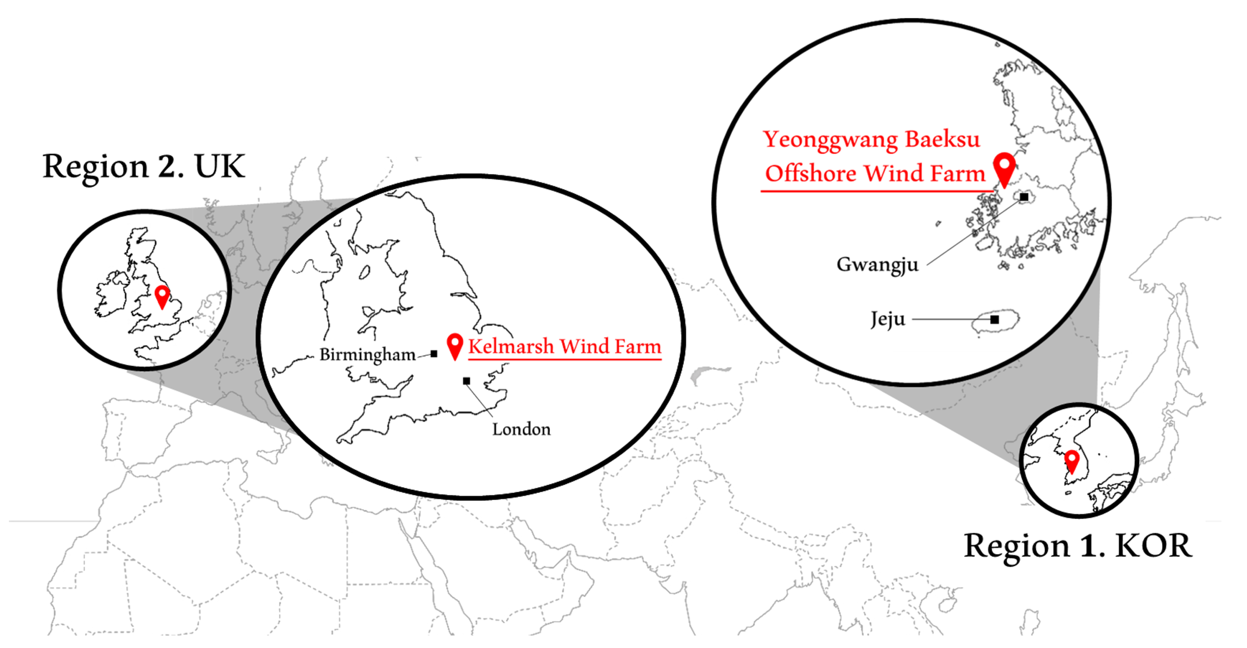
Data provided by two geographically distant wind power plants were used to verify the power generation prediction performance of each model as shown in Table 1. The place where the first dataset (hereinafter referred to as Data 1) was acquired was Yeonggwang Baeksu Wind Farm, located in Baeksu-eup, Yeonggwang-gun, Jeollanam-do, Korea, and Korea East-West Power provided data in the form of public data [26]. The data consist of power generation and wind speed data measured every 10 min for a total of one year from 1 January to 31 December 2020, from a 2.3 MW wind power generator by Unison. Power generation and wind speed are divided into three categories: minimum, average, and maximum; among them, average wind speed (m/s) and average power generation (kW) values are used in this paper. The second dataset (referred to as Data 2) was obtained from a wind farm in the Kelmarsh area of the UK. The wind farm data were provided by Cubico Sustainable Investments [27] and consist of 10 min data from 1 January to 31 December 2020 for one 2.05 MW rated turbine from Senvion. In the case of Data 2, data extracted from SCADA include information on the turbine state at that time or the connection with the system; however, in this paper, the average wind speed (m/s) and average power generation (kW) values were also used in Data 2 for meaningful comparison.

Table 1.
Basic data information.
3.1. Data Analysis
Figure 3 shows the location of the wind farm from which the data were acquired. Using the Pearson correlation coefficient, which quantifies the linear correlation between the two variables, the correlation coefficient based on the wind speed and power generation of each dataset is shown in Table 2 below.

Figure 3.
The location of the wind farm where the data were acquired.
Table 2.
Linear relationship between data expressed by the Pearson correlation coefficient.
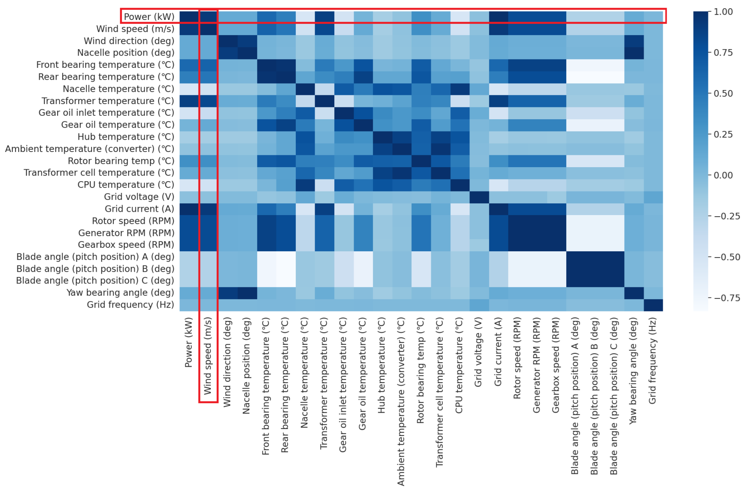
The Pearson correlation coefficient indicates that the closer the value is to absolute 1, the stronger the correlation. Due to the considerable distance between wind farms, the correlation between the two datasets is naturally weak, but there is a significant correlation between the wind speed measured and the power generation data within each wind farm. While Data 1 offers only wind speed (average, maximum, minimum) and power generation due to the limitations of public data, Data 2 provides SCADA data and records numerous data related to turbine operation. From Data 2, the Pearson correlation between each element and power generation is calculated as shown in Figure 4. In theory, wind speed has the greatest impact on wind power generation. However, assessing the relationship between wind speed and power generation simply by a linear relationship is challenging due to the numerous variables that affect power generation. Nevertheless, in the case of the input data utilized in this paper, the average wind speed was measured by instruments installed in the wind turbines, so it is estimated that the wind speed in each region played a dominant role in determining the power output of the respective wind farms.

Figure 4.
Pearson correlation coefficient for each element of Data 2.
Figure 5 shows the acquired data as wind speed on the x-axis and power generation on the y-axis. It can be seen that the distribution of the data is almost similar to the wind speed–power curve provided by each wind turbine manufacturer, and some measurements outside the curve can be classified as abnormal values. For example, in Data 1 of Figure 5a, there is a power generation amount smaller than 0, and values that do not match the wind speed–power curve are recorded from approximately 10 m/s to 17 m/s. Table 3 below lists the periods during which missing and abnormal data from Data 1 and Data 2 were recorded. In this paper, ‘missing’ means a case where the wind speed and power generation are suddenly recorded as 0, or a ‘nan’ value is acquired due to a measurement error.

Figure 5.
Wind Speed-Generation Curve. (a) Based on measured data. (b) Provided by the manufacturer.
Table 3.
Missing and abnormal period data.
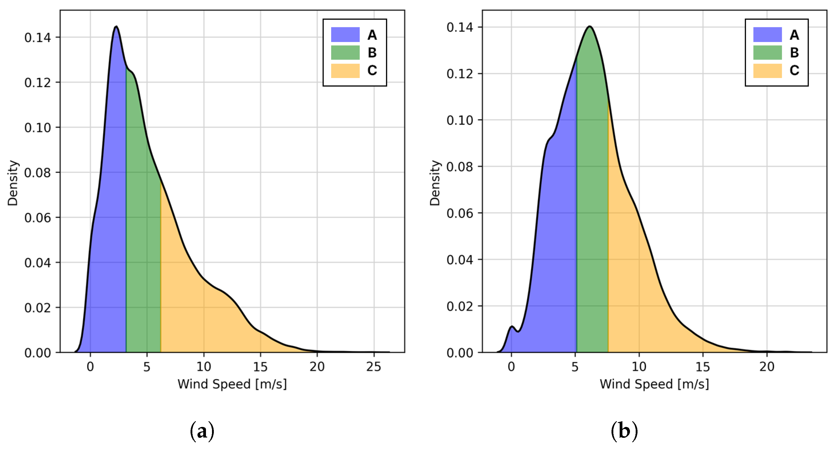
The wind speed distribution, represented by the KDE (kernel density estimation) graph, is shown in the black solid line in Figure 6 below. The measured wind speeds of the two datasets are distributed at values between 0 and 25 m/s; the maximum wind speed of Data 1 is about 25 m/s, which is larger than Data 2. Based on the wind speed value dividing the area of this KDE graph into three parts, the wind speed range of the area can be divided into the colored areas, A, B, and C, in Figure 6. Data 1 is divided into 3 m/s and 6 m/s, Data 2 is divided into 5 m/s and 8 m/s.

Figure 6.
The wind speed distribution. The wind speed distribution of each dataset is expressed by the KDE method. The graph is divided into A, B, and C, in three equal parts. The boundary wind speed values in each area are 3 m/s and 6 m/s in (a) of Data 1 and 5 m/s and 8 m/s in (b) of Data 2.
3.2. Data Preprocessing
Both datasets contain missing values and outliers. It was judged that missing values and outlier records due to measurement errors of the instrument could occur sufficiently in actual prediction situations, and that artificial interpolation could undermine the accuracy of the data because the missing periods were quite long. Therefore, outliers were not particularly treated, and all values were treated as 0 for periods with power generation less than zero and missing periods.
The columns of the dataset consist of wind speed and power generation, which correspond to the feature and target. In m/s and kW units, respectively, the feature and target are in different units. A normalization process before learning is required so that the difference in this range does not affect learning. For example, in the case of Data 1, the wind speed ranges from a minimum of 0 m/s to a maximum of 25.032 m/s, and the power generation ranges from a minimum of 0 to a maximum of 2357.924 kW. In order to eliminate the scale difference between these two items, they are converted to relative sizes: wind speed is normalized to be between 0 and 1 (from a range of 0 to 25.032) and power generation is normalized to be between 0 and 1 (from a range of 0 to 2357.924). Therefore, the feature and target were divided, and Min-Max normalization was applied to each dataset so that all data values fall between 0 and 1.
3.3. Feature Selection and Wind Speed-Based Data Classification: Proposed LGBM
In general, wind power generator data in the form of public data are often not provided with various items due to complex interests, such as the security and system operations of power generation companies. In the prediction, many elements can be used as features, including wind power generator operations, such as outside temperature and turbine rpm, as well as data representing system conditions, but items that are accessible to general users are limited. In this paper, only wind speed was used as a feature from the data to select the most suitable model for prediction based on the insufficient information on wind power generators.
For improved learning performance, forecast wind speed and previous power generation data were added as features along with wind speed. In the case of forecast wind speed, data were provided by the Meteorological Administration, but in this paper, the measured data were assumed to be the expected wind speed the next day. In addition, past generation data were used for the next day’s prediction process to emphasize the continuous time series features of the data; 70% of data were divided into a train set and 30% into a test set. Each dataset was converted and used according to the type of input required by the model layer.
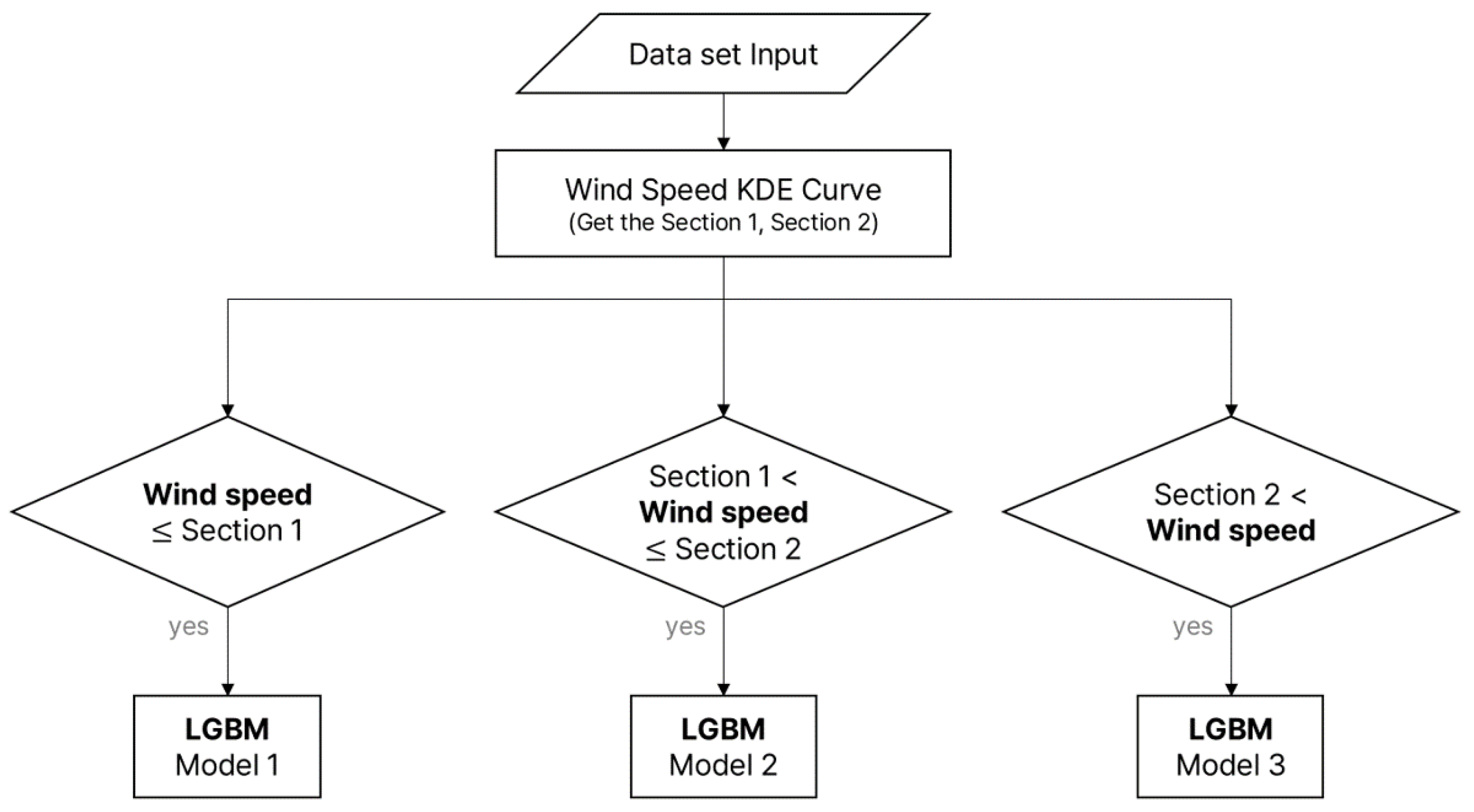
At this time, in the case of LGBM, due to the nature of the algorithm, the wind speed used for learning is past data, and the wind speed feature used for prediction corresponds to the forecast wind speed as it is. In order to further maximize the performance of the classification model, the input data of the LGBM model were divided by wind speed, classified using the KDE curve. That is, as shown in Figure 7, the data were divided into different models according to the wind speed criteria, and the data were configured to select and predict the model according to the section where the wind speed of the input test data corresponds.

Figure 7.
Proposed LGBM model prediction process by dividing the wind speed section.
4. Machine Learning Model and Parameters for Prediction
This paper compares the results of power generation prediction using three models, LSTM, CNN-biLSTM, and LGBM, which are mainly used for recent wind power generation prediction. Because time-measured wind speed and power generation data are used as inputs, LSTM, CNN-biLSTM corresponding to variations in LSTM, and LGBM, which have strengths in classification prediction, were selected as comparative groups. GPU computation was used in all prediction processes.
4.1. LSTM-Based
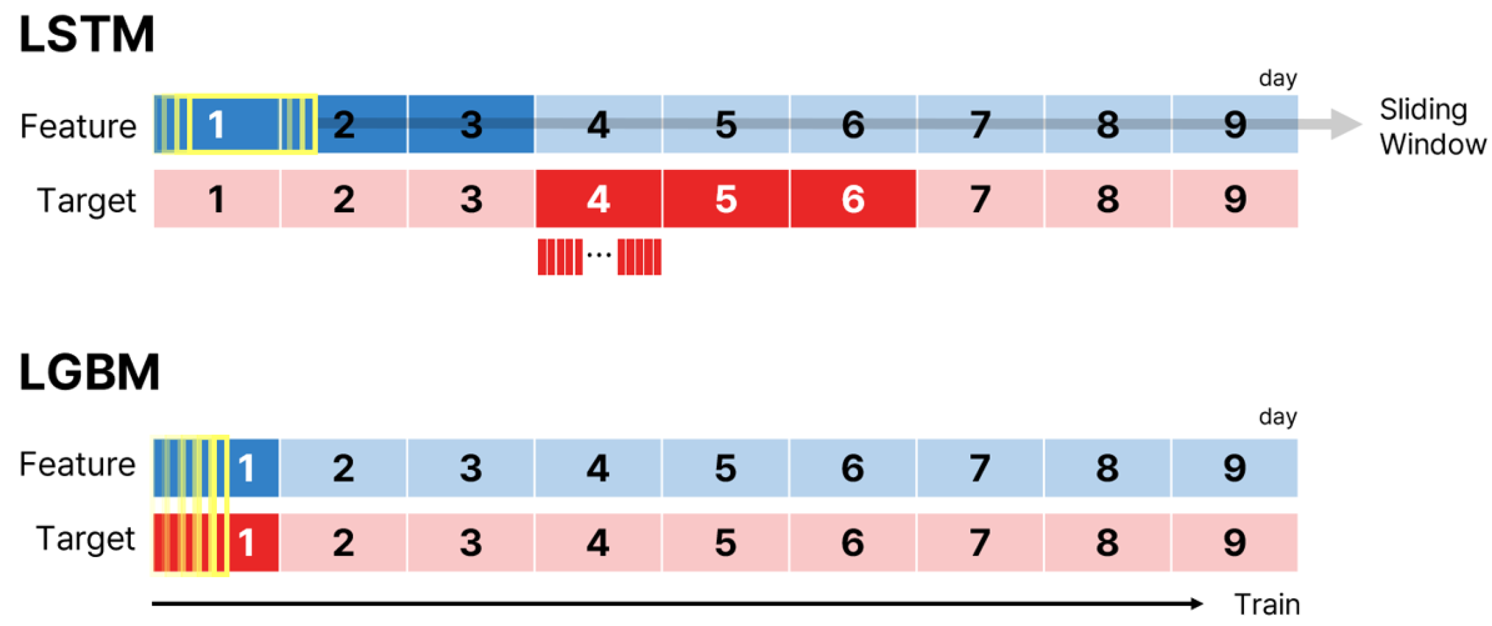
Two models, LSTM and CNN-biLSTM, used sliding window techniques to learn sequences separately, in order to use each dataset more efficiently as shown in Figure 8. Repeatedly separated time series data are learned according to the model layer configuration. In addition, to facilitate comparison between models, the remaining parameters were set the same, except for the layers added in CNN-biLSTM.

Figure 8.
Training process by models.
The LSTM model consists of two LSTM layers and two dense layers. Each layer selected the optimal parameters with heuristic techniques, and dropout was applied to prevent overfitting. In this paper, we also used CNN-biLSTM, which combines CNN with a bidirectional LSTM model known to perform better than LSTM. The model consists of seven hidden layers by changing the LSTM layer from the LSTM model to a bidirectional LSTM layer and adding two 1D convolutional layers and a MaxPooling layer to the front stage. It was intended to improve the nonlinear relationship learning performance between wind speed and power generation by combining a CNN model that is excellent in extracting features between features and an LSTM model that understands trends over time.
4.2. LGBM
LightGBM constructed a model using the regression model, LGBMRegressor. As described above, the model is learned by dividing data by wind speed to take advantage of the strength of the algorithm based on classification prediction. The hyperparameters of each wind speed model were set the same. In order to confirm the performance improvement effect of the model learning by classifying wind speeds, the classic LGBM model using all of the data was also selected as a comparative group.
4.3. Model Parameters
Due to the difference in the model structure used, this paper set parameters by dividing them into LSTM- and LGBM-based models. The parameters of each model are summarized in Table 4.
Table 4.
Model parameters.
First, in the case of the LSTM-based model, the number of layer nodes was set to decrease sequentially based on empirical methodology. The epoch and batch parameters, which have the highest effect on simulation time, were determined to be the maximum values that allowed the utmost utilization of the limited GPU capacity while learning all data within 2 hours. At the same time, it was assessed through a loss curve whether the chosen parameters were adequate for learning, and it was confirmed that the selected parameters were indeed appropriate. The window size for the sliding window method was set to 432, corresponding to a period of 3 days. This is because the model predicts the next day based on data from the past 3 days, and the window is shifted by one unit at a time.
Next, in the case of the LGBM model, the initial hyperparameters of the LGBM model were selected using flaml, which implements an AutoML process that automates repetitive machine learning model tuning. Subsequently, the final optimal hyperparameters were determined through an iterative process of trial and error.
5. Case Studies
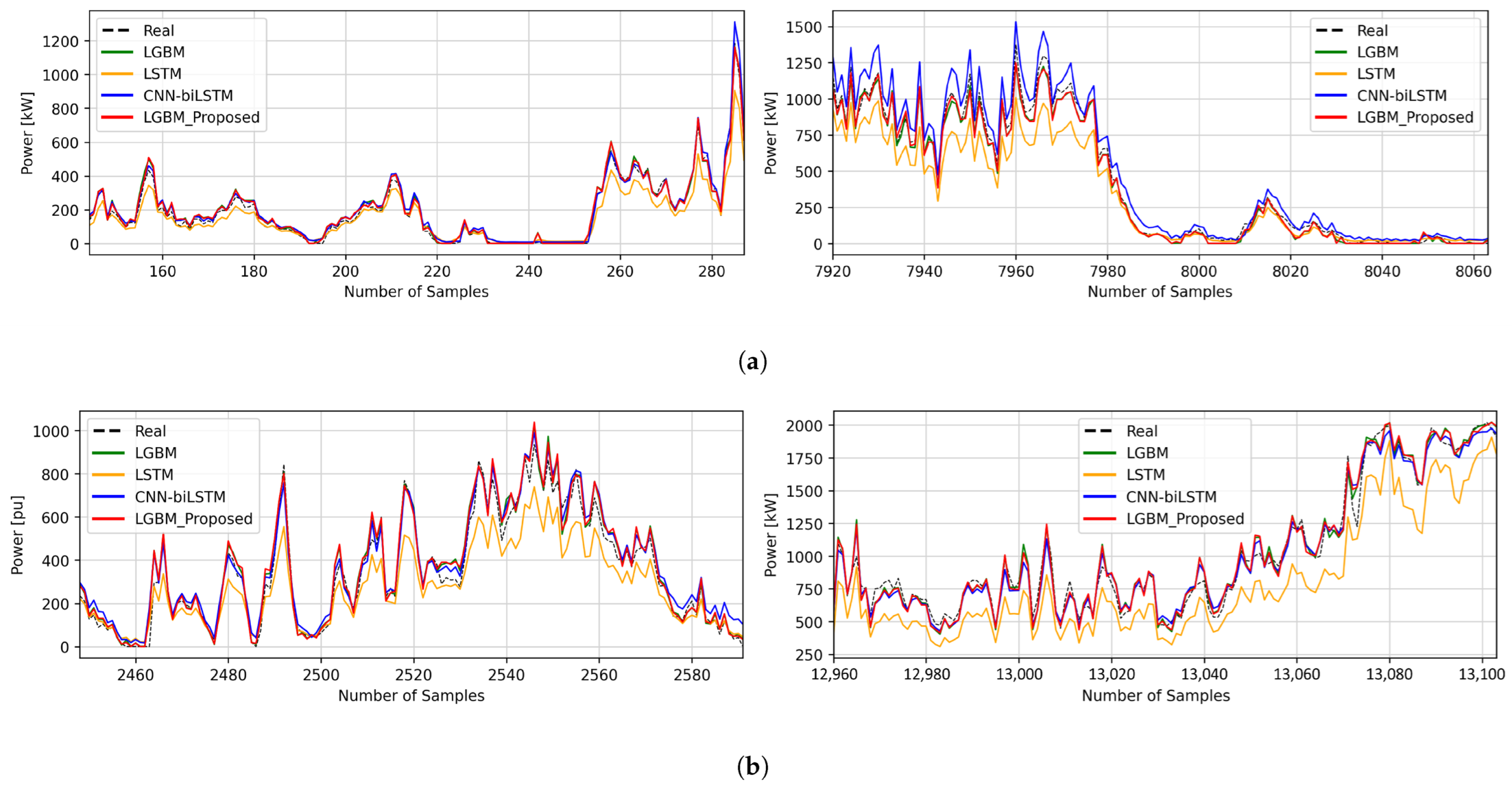
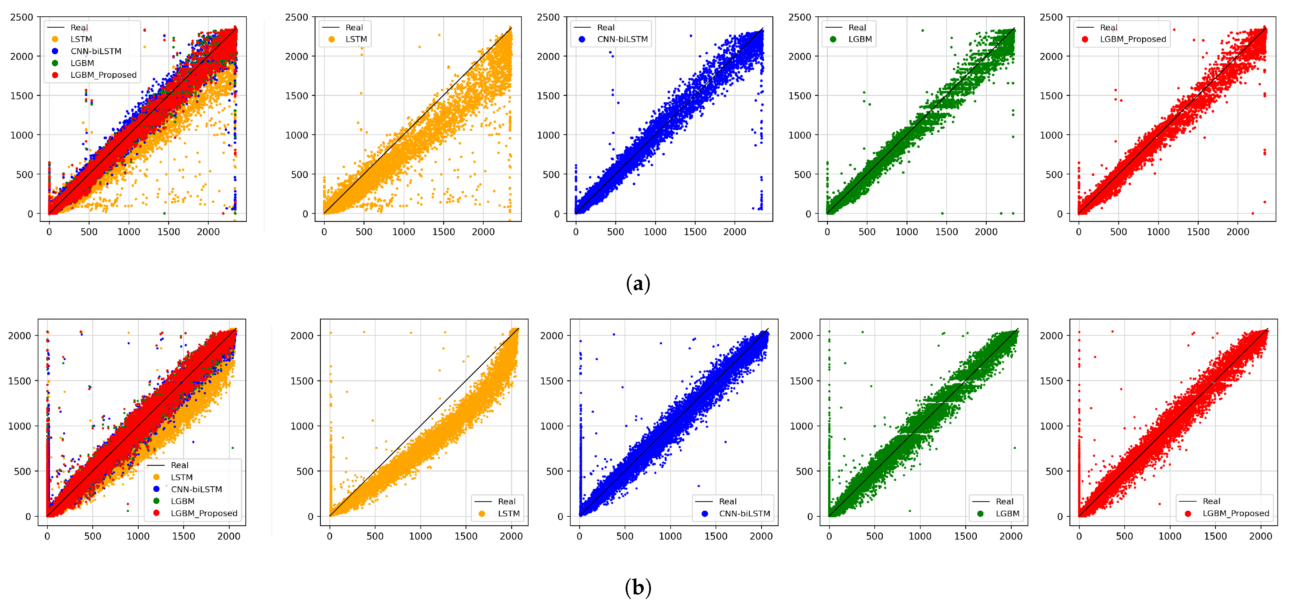
The model predicts output power over the next 24 h from inputs over the previous three days. Figure 9 shows a random two-day selection (144 points) of the prediction results for each model for Data 1 and Data 2, respectively; the amount of power generation corresponding to the correct answer value is indicated by a black line. Figure 10 shows the prediction results in a scatter plot.

Figure 9.
Graph of wind power output prediction results. (a) Data 1; (b) Data 2.

Figure 10.
Scatter plot of predicted results for each model. (a) Data 1; (b) Data 2.
RMSE (root mean square error) and (coefficient of determination), which are mainly used for time series prediction evaluation, were used as evaluation metrics of prediction accuracy. In the ith sample, when the predicted value is and the actual value is , the evaluation metrics are represented by Equations (1) and (2).
RMSE is a value obtained by averaging the square of the difference between the predicted value and the actual value, and is an indicator of the magnitude of the prediction error. RMSE means that the smaller the value, the higher the prediction accuracy. is an indicator of how well the prediction model explains the variation of the dependent variable; the closer it is to 1, the less the prediction error is.
6. Discussion
As a result of learning and predicting models for each dataset, it was confirmed that the proposed LGBM model, which divides data by wind speed, was the best at predicting wind power generation than other models. Likewise, the distribution of the proposed LGBM model’s prediction results was the most consistent with the actual value than other LSTM-based or LGBM models in the scatter plot, visually indicating how much the actual value and the predicted value are the same. Also, in the graph of the power generation prediction result of Figure 9, the prediction result of the proposed LGBM model, which applied classification by wind speed, was closest to the black dotted line representing the actual value. This was followed by the classic LGBM model, CNN-biLSTM, and LSTM in order of excellent prediction performance.
The wind turbine generator output is influenced by various variables and has nonlinear characteristics. However, when wind speed has a dominant effect on output, such as the data used in this paper, classification prediction according to wind speed is more appropriate than the LSTM-based methodology that attempts to grasp complex time-series relationships. In addition, the proposed LGBM model, which learns data based on wind speed through the wind speed distribution curve, performed better than the LGBM using all the data. The LGBM model generally prevents overfitting and increases the accuracy of classification prediction as the data increase, but the proposed LGBM model showed a smaller error despite the lack of overall data for learning. This suggests that if prediction is attempted with data where wind speed has a dominant effect on power generation, the approach of classifying data into large categories based on wind speed, as well as learning each of them in a separate model, can increase predictive performance.
The prediction error is summarized in Table 5 below.
Table 5.
Comparison of prediction errors by model and data.
7. Conclusions
In this paper, algorithms for predicting wind power generation were introduced, and the results of predicting power generation for each model were compared and analyzed using wind turbine public data obtained from Korea and the UK. This paper proposed a method to improve the wind power generation prediction performance by utilizing insufficient data, especially when various features were not provided. When wind speed was highly related to output power, such as the data used in the paper, the decision tree model LGBM showed better prediction performance than LSTM-based algorithms, which are known for their excellence in time series prediction. In addition, the proposed LGBM model, which classified data according to the wind speed section based on the wind speed distribution, had better prediction performance than the LGBM model, which used all of the existing data.
The results of this study are expected to be used to construct ensemble models combined with various other algorithms or to help wind generator operators select and organize prediction algorithms that will participate in incentive systems based on prediction accuracy. In the future, it is expected that prediction accuracy will be further improved if various weather observation data, including wind speed, can be acquired as features, or larger amounts of past data can be used for learning.
Author Contributions
Conceptualization, H.L. and M.Y.; Methodology, S.I., H.L., D.H. and M.Y.; Software, H.L.; Validation, D.H. and M.Y.; Writing—original draft, S.I.; Writing—review & editing, D.H. and M.Y.; Visualization, S.I.; Supervision, D.H. and M.Y. All authors have read and agreed to the published version of the manuscript.
Funding
This work was supported by the Korea Institute of Energy Technology Evaluation and Planning (KETEP) grant funded by the Korean government (MOTIE) (no. 20223030020110) and the Korea Electric Power Corporation grant (R22XO05-02).
Conflicts of Interest
The authors declare no conflict of interest.
Abbreviations
The following abbreviations are used in this manuscript:
| LSTM | long short-term memory |
| CNN-biLSTM | convolutional neural network-bidirectional LSTM |
| LGBM | light gradient boosting machine |
| ARIMA | autoregressive integrated moving average |
| KEPCO | Korea Electric Power Corporation |
| RNN | recurrent neural network |
| KDE | kernel density estimation |
| RMSE | root mean square error |
References
- International Energy Agency. Renewable Energy Market Update; Report; International Energy Agency: Paris, France, 2023.
- International Energy Agency. World Energy Outlook 2022; Report; International Energy Agency: Paris, France, 2022.
- UK Goverment. Powering up Britain; Policy Report; Department for Energy Security and Net Zero: Westminster, UK, 2023. Available online: https://www.gov.uk/government/publications/powering-up-britain (accessed on 23 June 2023).
- European Commission. REPowerEU: Affordable, Secure and Sustainable Energy for Europe; Policy Report; European Commission: Makati, PH, USA, 2022.
- European Commission. Fit for 55: Delivering the EU’s 2030 Climate Target on the Way to Climate Neutrality; Policy Report; European Commission: Makati, PH, USA, 2021.
- Korea Power Exchange. Electric Power Statistics Information System. 2023. Available online: https://epsis.kpx.or.kr/epsisnew/selectMain.do?locale=eng (accessed on 23 June 2023).
- 2050 Presidential Commission on Carbon Neutrality and Green Growth. 2030 Nationally Determined Contributions; Policy Report; The Presidential Commission on Carbon Neutrality and Green Growth: Sejong-si, Republic of Korea, 2021.
- Wei, J.; Zhang, Y.; Wang, J.; Cao, X.; Khan, M.A. Multi-period planning of multi-energy microgrid with multi-type uncertainties using chance constrained information gap decision method. Appl. Energy 2020, 260, 114188. [Google Scholar] [CrossRef]
- Lane Clark & Peacock LLP. Renewable Curtailment and the Role of Long Duration Storage; Report; Lane Clark & Peacock LLP: London, UK, 2022. [Google Scholar]
- Korea Power Exchange. Monthly and Hourly Jeju Solar Wind Power Control Amount and Number of Control; Statistics; Korea Power Exchange: Naju-si, Republic of Korea, 2023. [Google Scholar]
- Korea Power Exchange. Electricity Market Operation Rules, Renewable Energy Generation Prediction System; Statistics; Korea Power Exchange: Naju-si, Republic of Korea, 2022. [Google Scholar]
- Kavasseri, R.G.; Seetharaman, K. Day-ahead wind speed forecasting using f-ARIMA models. Renew. Energy 2009, 34, 1388–1393. [Google Scholar] [CrossRef]
- Palomares-Salas, J.C.; Rosa, J.J.D.L.; Ramiro, J.G.; Melgar, J.; Agüera, A.; Moreno, A. ARIMA vs. neural networks for wind speed forecasting. In Proceedings of the 2009 IEEE International Conference on Computational Intelligence for Measurement Systems and Applications, CIMSA 2009, Hong Kong, China, 11–13 May 2009. [Google Scholar] [CrossRef]
- Xu, Q.; Li, W.; Kong, D.; Zhao, X.; Wang, X.; Li, Y.; Shen, Y.; Wang, X.; Zhao, Z. Ultra-short-term wind speed forecast based on WD-ARIMAX-GARCH model. In Proceedings of the 2019 IEEE 2nd International Conference on Automation, Electronics and Electrical Engineering, AUTEEE 2019, Shenyang, China, 22–24 November 2019. [Google Scholar] [CrossRef]
- Krechowicz, A.; Krechowicz, M.; Poczeta, K. Machine Learning Approaches to Predict Electricity Production from Renewable Energy Sources. Energies 2022, 15, 9146. [Google Scholar] [CrossRef]
- Baek, J.; Park, S.; Choi, S.; Kim, H. Renewable Forecasting Method for Local Renewable Management System. Trans. Korean Inst. Electr. Eng. 2022, 71, 1062–1069. [Google Scholar] [CrossRef]
- Yebin, L.; Sangho, P.; Jin, H. A Study on Wind Power Output Forecasting Model Using Deep Learning Approach Based on CNN. In Proceedings of the 53th KIEE Summer Conference 2022, Yeosu, Republic of Korea, 13–16 July 2022. [Google Scholar]
- Minju, L.; Solyoung, J.; Jaegul, L.; Jin, H. A Short-term Wind Power Output Forecasting based on R-LSTM Algorithm. In Proceedings of the 53th KIEE Summer Conference 2022, Yeosu, Republic of Korea, 13–16 July 2022. [Google Scholar]
- Ren, J.; Yu, Z.; Gao, G.; Yu, G.; Yu, J. A CNN-LSTM-LightGBM based short-term wind power prediction method based on attention mechanism. Energy Rep. 2022, 8, 437–443. [Google Scholar] [CrossRef]
- Dongmin, B. A Study on the Prediction Errors Reduction Algorithm of the YEONGGWANG Wind Power Generation Based on Big Data. Master’s Thesis, Hanyang University, Seoul, Republic of Korea, 2022. [Google Scholar]
- Jung, A.H.; Lee, D.H.; Kim, J.Y.; Kim, C.K.; Kim, H.G.; Lee, Y.S. Regional Photovoltaic Power Forecasting Using Vector Autoregression Model in South Korea. Energies 2022, 15, 7853. [Google Scholar] [CrossRef]
- Chang, W.Y. A Literature Review of Wind Forecasting Methods. J. Power Energy Eng. 2014, 2, 161. [Google Scholar] [CrossRef]
- Jahangir, H.; Tayarani, H.; Gougheri, S.S.; Golkar, M.A.; Ahmadian, A.; Elkamel, A. Deep Learning-Based Forecasting Approach in Smart Grids with Microclustering and Bidirectional LSTM Network. IEEE Trans. Ind. Electron. 2021, 68, 8298–8309. [Google Scholar] [CrossRef]
- Kim, T.Y.; Cho, S.B. Predicting residential energy consumption using CNN-LSTM neural networks. Energy 2019, 182, 72–81. [Google Scholar] [CrossRef]
- Ke, G.; Meng, Q.; Finley, T.; Wang, T.; Chen, W.; Ma, W.; Ye, Q.; Liu, T.Y. LightGBM: A highly efficient gradient boosting decision tree. In Proceedings of the 31st Conference on Neural Information Processing Systems (NIPS 2017), Long Beach, CA, USA, 4–9 December 2017. [Google Scholar]
- Korea East-West Power. Yeonggwang Baeksu Wind Farm Unit 1 10-Minute Average Power Generation. 2022. Available online: https://www.data.go.kr/data/15091978/fileData.do (accessed on 23 June 2023).
- Plumley, C. Kelmarsh Wind Farm Data. 2022. Available online: https://zenodo.org/record/5841834 (accessed on 23 June 2023). [CrossRef]


Disclaimer/Publisher’s Note: The statements, opinions and data contained in all publications are solely those of the individual author(s) and contributor(s) and not of MDPI and/or the editor(s). MDPI and/or the editor(s) disclaim responsibility for any injury to people or property resulting from any ideas, methods, instructions or products referred to in the content. |
© 2023 by the authors. Licensee MDPI, Basel, Switzerland. This article is an open access article distributed under the terms and conditions of the Creative Commons Attribution (CC BY) license (https://creativecommons.org/licenses/by/4.0/).