Multi-Angle Reliability Evaluation of Grid-Connected Wind Farms with Energy Storage Based on Latin Hypercube Important Sampling

Abstract

Aiming to combat the problems of slow speed and poor accuracy of reliability evaluation of the power system in wind farms with energy storage, this paper proposes a method of reliability evaluation based on Latin hypercube important sampling (LHIS). Firstly, we aimed to establish the Latin hypercube important sampling evaluation model by combining the Latin hypercube sampling method with the important sampling method. Secondly, we aimed to optimize the sample probability distribution of the components and conduct hierarchical sampling of the system. Then, the comprehensive risk indicator (CRI) was proposed to evaluate the operational risk and the wind storage generation interrupted energy benefit (WSGIEB) was proposed to evaluate the contribution of the reliability. Finally, simulation experiments were carried out through various power system operation scenarios. The simulation results show that the proposed method is 47% higher than the improving importance sampling method (IM-IS) in evaluation speed and 33% higher than the improving importance sampling method in calculation accuracy.

1. Introduction

Energy storage systems can improve the fluctuation of wind farm output; however, the operation conditions of the wind turbines and energy storage systems, the energy storage capacity and charging and discharging strategy, the wind power access capacity, and so on, will affect the reliability of the power system to varying degrees. Therefore, it is of great significance to study how to accurately evaluate the reliability of grid-connected wind farms with energy storage systems under different operating conditions for the stable operation of the grid under the background of the high proportion of wind power access [1]. The key to the accuracy of power grid reliability evaluation of wind farms and energy storage systems lies in selecting the power grid reliability evaluation method and constructing the evaluation index.

Aiming toward the selection of evaluation methods, early power system reliability evaluation mainly relied on the analytical method, whose computational complexity depended on the complexity of the power system solution space. However, as a large number of renewable energy sources were connected to the grid, the random variables in the system increased greatly, and their correlation structures became more and more complex. Therefore, the bottleneck of traditional analytical methods cannot be completely solved. Therefore, the simulation method of reliability evaluation based on Monte Carlo sampling (MCS) has received much attention [2,3]. Li. [4] used the sequential Monte Carlo method and the non-sequential Monte Carlo method to evaluate the power system and compared the advantages and disadvantages of the two methods. Zhao et al. [5] used the cross-entropy method to optimize the non-sequential Monte Carlo method, which improved the efficiency of evaluation calculation. However, there was still a problem of non-representativeness of samples.

Although, in theory, as long as the sample size is large enough, the reliability index obtained by the MCS method will be infinitely close to the real value. But the reliability evaluation of large-scale high-reliability power systems will have a long calculation cycle. Therefore, it is necessary to optimize the sampling method and improve the ability of the sample to characterize the probability distribution. The Latin hypercube sampling (LHS) method combines random sampling with stratified sampling, which improves the representation ability of samples on the overall probability distribution [6]. Huang et al. [7] proposed the LHS probabilistic power flow algorithm based on Gram–Schmidt sequence orthogonalization, which effectively improved the sampling efficiency and reduced the variance of the estimator.

However, the above methods only optimized the sampling method. In order to minimize the sample size as much as possible, the prominent research involved the combination of sampling methods with various variance reduction methods, among which the importance sampling method had the most significant effect [8]. Tómasson et al. [9] proposed a reliability assessment method for composite power systems based on important sampling (IS), which was superior to the cross-entropy algorithm, but the sampling method was more complex and reduced the sampling efficiency. Cai et al. [10] combined the IS method with multinomial distribution in order to achieve dimensionality reduction in random variables. LHS can optimize the sampling methods, while IS can optimize probability distribution; however, the aforementioned scholars did not consider combining the two methods. Zhang et al. [11] proposed the EV-LHS method, which first used the importance concept to reduce the sample size, and then sampled based on the LHS method. However, this method did not consider the issue of reducing sample correlation. At present, the reliability of the power grid of wind farms and energy storage systems is mostly evaluated by the Monte Carlo simulation method with simple sampling, and there are still some shortcomings, such as poor convergence and low accuracy. To solve this problem, this paper first optimizes the probability distribution of the sampling objects using the IS method and then combines the LHS method to stratified sample system components. The two methods are organically combined to propose the LHIS method.

Aiming toward the construction of an evaluation index, most scholars based their work on the traditional power grid reliability index. Ungjin et al. [12,13] calculated the frequency of an insufficient power supply, and the power shortage time expectation and power shortage expectation were calculated in order to evaluate the grid reliability. From the perspective of economic risk, the expected value of electricity cost loss and economic loss was proposed in [14] in order to evaluate the grid reliability after the wind farms and energy storage systems were connected. Yang et al. [15,16] carried out a power grid reliability assessment from power deficit expectation indexes considering different energy storage control strategies and constraints. With the goal of improving the contribution of energy storage batteries to system reliability, the expected power shortage was calculated in [17] to evaluate the reliability of the power grid, and the optimal operation strategy of energy storage systems was provided. However, the above research lacks the risk analysis of the power system and does not consider the severity of the consequences caused by this situation.

In view of the above problems, this paper evaluates the reliability of the power system in wind farms and storage systems from two aspects based on Latin hypercube important sampling (LHIS). Firstly, the spatial probability distribution of sampling objects is optimized based on the IS method, and then the system components are sampled in layers by combining them with the LHS method. The LHIS method is put forward by combining the two methods organically. Then, the comprehensive risk indicator (R_CRI) and the wind storage generation interrupted energy benefit (WSGIEB) are constructed in order to evaluate the reliability of the power system. Finally, a variety of differentiated power grid operation scenarios are set up to verify the effectiveness of the proposed method. The results of one example show that this method can effectively evaluate the reliability of the grid after the wind power and storage systems are connected to the system and provide a useful reference for the design and dispatch strategy of the power system of wind farms and energy storage systems.

The main contributions of this paper are as follows:

(1)

To solve the issues of poor convergence and low accuracy of grid reliability evaluation of wind farms and energy storage, this paper proposes a power system reliability evaluation method based on LHIS. First, the sample space probability distribution of the sample object is optimized, and the optimized probability distribution is stratified sampled. Then, the correlation of the sampling matrix is reduced.

(2)

To solve the problem of the lack of risk analysis and the severity of the consequences in the case, this paper evaluates the power grid from two perspectives: the operational risk and the contribution to system reliability. Three operation scenarios are set for connecting wind farms with energy storage systems at different nodes, connecting wind farms of different capacities with energy storage systems, and connecting wind farms with different energy storage capacities. It has been verified that the method can evaluate the reliability of the grid more comprehensively and accurately.

The other parts of this paper are arranged as follows: Section 2 introduces the wind farm output model. Section 3 establishes the LHIS evaluation model and provides the specific evaluation process then defines the evaluation indicators. In Section 4, the LHIS method is compared with LHS method and IM-IS method in order to verify the efficiency and universality of this method. Simultaneously, the different power system connection modes based on the LHIS method are simulated and analyzed. Finally, Section 5 ends the paper by summarizing the main conclusions.

2. Wind Farm Output Model

The statistics on a large amount of wind speed data show that the Weibull distribution of two parameters can describe the variation law of wind speed. This distribution is represented by Formula (1) [18]:

$$F(v)=1-e^{-{\left(\frac{v}{\lambda }\right)}^k}$$

(1)

The distribution function is expressed by Formula (2):

$$f(v)=\frac{k}{\lambda }{\left(\frac{v}{\lambda }\right)}^{k-1}{e}^{-{\left(\frac{v}{\lambda }\right)}^k}$$

(2)

where $\lambda$ is the scale parameter, representing the average wind speed of the wind farms, $v$ is the wind speed value, and $k$ is the shape parameter.

The probability sampling value of wind speed can be obtained by changing the distribution function, and the distribution function is transformed into the following:

$$v=\lambda {[-\ln (1-x)]}^{\frac{1}{k}}$$

(3)

Because the range of $1-x$ and x in the formula is $[0,1]$, the distribution function can be rewritten as follows:

$$v=\lambda {[-\ln (x)]}^{\frac{1}{k}}$$

(4)

The relationship between the fan output power and the wind speed can be expressed by formula [19], as follows:

$$P_t\left(v\right)=\{\begin{array}{ll}0\hfill & (v<v_{ci})\cup (v>v_{co})\hfill \\ \frac{v^3-v_{ci}^3}{v_r-v_{ci}^3}{P}_{WR}\hfill & v_{ci}\le v\le v_r\hfill \\ P_{WR}\hfill & v_r<v\le v_{co}\hfill \end{array}$$

(5)

where $P_t(v)$ is the real-time output power of the fan; $v_{ci}$ and $v_{co}$ are the cut-in wind speed and the cut-out wind speed of the fan, respectively; and $v_r$ is the rated wind speed.

3. Reliability Evaluation for Power Systems with Wind Farms and Energy Storage Systems Based on the Latin Hypercube Importance Sampling Method

3.1. Charge and Discharge Model of Energy Storage System

According to the output and load of the wind farm, there are two charging and discharging strategies of the energy storage system.

Strategy 1: When the output of the wind farm is less than $P_L(t)·\eta$, the energy storage system begins to discharge. In order to limit the output power of the wind farm and the energy storage system, it is required that the sum of the output of the wind farm and the energy storage battery should not exceed $P_L(t)·\eta$. The discharge power of the energy storage battery is expressed as follows [20,21]:

$$P_d(t)=\min (P_L(t)·\eta -P_W(t),P_{disch}^{\max })$$

(6)

where $P_{disch}^{\max }$ represents the maximum discharge power of the energy storage system, $\eta$ is the wind power permeability, $P_W(t)$ is the power generated by the wind farm, and $P_L(t)$ is the maximum load of the system. When the output of the wind turbine is greater than $P_L(t)·\eta$, the energy storage system begins to charge. The charging power of the energy storage system is expressed as follows:

$$P_c(t)=\min (P_W(t)-P_L(t)·\eta ,P_{ch}^{\max })$$

(7)

where $P_{ch}^{\max }$ represents the maximum charging power of the energy storage battery.

Strategy 2: When the output of the wind farm is less than $P_L(t)·\eta$, and the output of the conventional power plant cannot meet the demand of the residual load, the energy storage system starts to discharge. The discharge power of the energy storage system is expressed as follows [20,21]:

$$P_d(t)=\min (P_L(t)·\eta -P_W(t),P_L(t)-P_W(t)-P_D(t),P_{disch}^{\max })$$

(8)

When the output of the wind farm is greater than $P_L(t)·\eta$, the energy storage system begins to charge. The charging power of the energy storage battery is expressed in Formula (7).

3.2. Latin Hypercube Important Sampling (LHIS)

Latin hypercube sampling (LHS) adopts a stratified sampling method, which can effectively reflect the overall distribution of the random variables through sampling values [7]; however, the sampling method of Latin hypercube sampling at the tail of probability density function will affect the accuracy of the algorithm. In this paper, the LHIS method is established by combining the LHS method with the IS method.

3.2.1. Sampling Principle

The LHIS method is carried out as follows: Firstly, the probability distribution of the sample space of the sampling object is optimized based on the IS method. Then, the optimized probability distribution is sampled by the LHS method. Finally, the correlation of the sampling matrix is reduced by the Cholesky decomposition method. The specific steps are as follows:

(1)

Optimize the spatial probability distribution of the sampling objects based on the IS method. Then, make the mathematical expectation $E(X)$ of the original sample of the sampling object unchanged and replace the original sample space probability distribution $P(X)$ with the new probability distribution $P^{\ast }(X)$. If the new variance is 0, then the $P_{\mathrm{op}}^{\ast }(X)$ is the optimal probability distribution at this time. The method is as follows [22]:

$$P^{\ast }(X)=\frac{F(X)}{E(F)}P(X)=P_{\mathrm{op}}^{\ast }(X)$$

(9)

where $F(X)$ is the sampling function and $E(F)$ is the sampling expectation value. Because it cannot be determined in the sampling process, the probability distribution of the optimized sample space can only be approximately optimal. From Formula (9), $P^{\ast }(X)$ is proportional to $P(X)$, let m be the proportional coefficient, then Formula (9) is rewritten as: $P^{\ast }(X)=mP(X)$.

Let a component i in the power system have a sample space probability distribution of $P(X^i)$, and take the optimal multiplier, γ, of the intermediate variable to construct its new probability distribution, $P^{\ast }(X^i)$, as shown in formula [23], as follows:

$$P^{\ast }\left(X^i\right)=\{\begin{array}{ll}\gamma {\lambda }_i\hfill & X^i=1(\mathrm{breakdown})\hfill \\ 1-\gamma {\lambda }_i\hfill & X^i=0(\mathrm{operation})\hfill \end{array}$$

(10)

Therefore, the problem of calculating the proportional coefficient, m, to obtain the approximate optimal probability distribution is transformed into the problem of finding the optimal multiplier, γ. The calculation formula of the proportional coefficient, m, is as follows [24]:

$$m=\frac{P^{\ast }(X)}{P(X)}={\displaystyle \prod _{i=1}^{n_1}\gamma }{\displaystyle \prod _{i=1}^{n_0}\frac{1-\gamma {\lambda }_i}{1-{\lambda }_i}}$$

(11)

where $n_1$ is the number of faulty components in the sampling process and $n_0$ is the number of running components.

Based on the iterative method, γ is calculated. Firstly, it is given an initial value, and then iterated through small-scale sampling until the adjacent γ reaches the specified relative error accuracy. The calculation formula is as follows [24]:

$$\gamma =-\frac{B+\sqrt{B^2-AC}}{A}$$

(12)

$$\{\begin{array}{l}A=\frac{n_1}{n_0+n_1}\overline{\lambda }-\left(1-\frac{n_1}{n_0+n_1}\right)\overline{\lambda }(1-\overline{\lambda })\hfill \\ B=-\frac{n_1}{n_0+n_1}\overline{\lambda }\hfill \\ C=\frac{n_1}{n_0+n_1}\hfill \\ \overline{\lambda }=\frac{1}{n}{\displaystyle \sum _{i=1}^n{\lambda }_i}\hfill \end{array}$$

(13)

where $A$, $B$, and $C$ are the calculation coefficients and $\overline{\lambda }$ the average failure rate of the components.

(2)

Sample the optimized probability distribution based on the LHS method. Stratify the input random variables and select the random sampling points in each hypercube as the sampling points, according to the importance shown in the original probability density function, usually the boundary of the hypercube closest to the expected value. The calculation formula of $X_{kn}$ is as follows (assuming that the sampling number, $n$, is even) [11]:

$$X_{kn}=\{\begin{array}{ll}{F}_k^{-1}(n/N)\hfill & n/N\le 0.5\hfill \\ F_k^{-1}((n-1)/N)\hfill & n/N>0.5\hfill \end{array}$$

(14)

The LHIS method comprehensively considers the two ideas of “stratification” and “importance” in sampling, which makes the sampled points closer to the expected value and accelerates the convergence of LHIS.

(3)

Reduce the correlation of the sampling matrix based on the Cholesky decomposition method. If K components are sampled, and the sampling times of each component is N, then all of the sampled values will form an initial sampling matrix, $X_{KN}$, of order $K\times N$. The accuracy of the evaluation results is greatly affected by the correlation of the sampled values in the sampling matrix, therefore, the correlation between the lines of the sampling matrix should be reduced.

Firstly, construct an arrangement matrix, $L_{KN}$, and the element value of each row will represent the arrangement position of the corresponding row elements in each row in the $X_{KN}$.

Then, construct the row correlation coefficient matrix ${\rho }_L$ of the $L_{KN}$. ${\rho }_L$ is a matrix of $K\times K$ order, in which the elements are the correlation coefficients between each row, which can be expressed as follows [25]:

$${\rho }_{ij}=\frac{{\displaystyle \sum _{k=1}^K\left[\left(V_{ik}-\overline{V_i}\right)\left(V_{jk}-\overline{V_j}\right)\right]}}{\sqrt{{\displaystyle \sum _{k=1}^K{\left(V_{ik}-\overline{V_i}\right)}^2{\displaystyle \sum _{k=1}^K{\left(V_{jk}-\overline{V_j}\right)}^2}}}}$$

(15)

Obtain the lower triangular matrix, D, by the Cholesky decomposition method, and then construct a matrix with less correlation, $G_{KN}$, by combining the D matrix, which can be expressed as follows [25]:

$${\rho }_L=D{D}^T$$

(16)

$$G_{KN}=D^{-1}{L}_{KN}$$

(17)

Finally, rearrange the elements in the $X_{KN}$ according to the $G_{KN}$ from the largest to the smallest, and repeat the above steps until the $L_{KN}$ is less than the required value.

3.2.2. Sampling the Power Systems with Wind Farms and Storage Systems

Sample the distribution function (2) based on the LHIS method and obtain the n-th wind speed sampling value as follows:

$$v_n=\{\begin{array}{c}\lambda {\left[-\ln \left(F_k^{-1}(n/N)\right)\right]}^{\frac{1}{k}} n/N\le 0.5\\ {\lambda \left[-\ln \left(F_k^{-1}((n-1)/N)\right)\right)]}^{\frac{1}{k}}n/N>0.5\end{array}$$

(18)

Considering the influence of the wake effect, construct the sampling matrix sequence of the wind speed by completing the set N sampling times, as follows [26]:

$$V_W=\left[v_1,v_2,\cdots ,v_n,\cdots ,v_N\right]$$

(19)

Based on the failure rate and repair rate of the fan, obtain the distribution function of the fan state as follows:

$$Y_{\mathrm{WT}}=\{\begin{array}{ll}\frac{\left(1-P_{d0}-P_{f0}\right)\left(X_{\mathrm{WT}}-b\right)}{c-b}+P_{f0}+P_{d0}\hfill & X_{\mathrm{WT}}\in [b,c)\hfill \\ \frac{P_{f0}\left(X_{\mathrm{WT}}-a\right)}{b-a}+P_{d0}\hfill & X_{\mathrm{WT}}\in [a,b)\hfill \\ \frac{X_{\mathrm{WT}}{P}_{d0}}{a}\hfill & X_{\mathrm{WT}}\in [0,a)\hfill \end{array}$$

(20)

By sampling Equation (20) N times by LHIS method, obtain the sampling matrix sequence of the wind turbine state as follows:

$$X_{WT}=\left[X_{WT-1},X_{WT-2},\cdots ,X_{WT-n},\cdots X_{WT-N}\right]$$

(21)

Then, obtain the initial sampling matrix, $X_{KN}$, after sampling the power system with the wind farm and energy storage system N times, which can be expressed as follows:

$$X_{KN}=[V_W,X_{WT1},\cdots ,X_{WTi},X_{G1},\cdots ,X_{Gg},X_{T1},\cdots ,X_{Tk}, {X_{L1},\cdots ,X_{Lm},X_{ES1},\cdots ,X_{ESp}]}^T$$

(22)

In the formula, $X_{WTi}$, $X_{Gg}$, $X_{Tk}$, $X_{ESp}$, and $X_{Lm}$ are, respectively, represented as sampling vector groups that sample wind turbines, conventional generators, transformers, lines, and energy storage systems N times, where $i+g+k+m+p+1=K$.

The correlation between the sampling values of each row of $X_{KN}$ is large, therefore, it is necessary to rearrange $X_{KN}$ according to $L_{KN}$, as proposed in Section 3.2.1, to reduce the correlation of $X_{KN}$.

3.3. Evaluation Indicators

To analyze the influence of wind storage systems on the power grid comprehensively, comprehensive evaluation indexes are needed in order to reflect the situation of the power grid. In this paper, a comprehensive risk index ($R_{CRI}$) [27,28] and the wind storage generation interrupted energy benefit (WSGIEB) are used as evaluation indicators.

3.3.1. Comprehensive Risk Indicator ($R_{CRI}$)

Considering the evaluation results of the risk of load cutting, $R_{CUT}$, the risk of line active power exceedance, $R_{LINE}$, and the risk of voltage exceedance, $R_V$, the comprehensive risk index, $R_{CRI}$, is proposed, which can be expressed as follows [29]:

$$R_{CRI}={\omega }_1{R}_{CUT}+{\omega }_2{R}_{LINE}+{\omega }_3{R}_V$$

(23)

In the formula, ${\omega }_1$, ${\omega }_2$, and ${\omega }_3$ are the weights of the above three risk indicators, which can be obtained by the analytic hierarchy process. The $R_{CUT}$ represents the risk of load cutting under certain operating conditions of the system. The lower the risk number, the more reliable the system. The $R_{LINE}$ represents the risk of the line active power exceeding the maximum allowable active power under a certain operating condition. The $R_V$ represents the risk of voltage exceedance of the upper or lower limit under a certain operating condition. The calculation formula of $R_{CUT}$, $R_{LINE}$, and $R_V$ is as follows [29]:

$$\{\begin{array}{l}{R}_{CUT}={\displaystyle \sum _{k=1}^K{p}_{wt}}\left(E_k\right)p_g\left(E_k\right)p_{ling}\left(E_k\right)p_{es}\left(E_k\right) S_{ev-CUT}\left(E_k\right)\hfill \\ \begin{array}{l}{R}_{LINE}={\displaystyle \sum _{k=1}^K{p}_{ut}}\left(E_k\right)p_{ge}\left(E_k\right)p_{line}\left(E_k\right)p_{es}\left(E_k\right)S_{ev-LINE}\left(E_k\right)\\ R_V={\displaystyle \sum _{k=1}^K{p}_{wt}}\left(E_k\right)p_{ge}\left(E_k\right)p_{lme}\left(E_k\right)p_{es}\left(E_k\right)S_{ev-V}\left(E_k\right)\end{array}\hfill \end{array}$$

(24)

where $p_{wt}\left(E_k\right)$, $p_g\left(E_k\right)$, $p_{ling}\left(E_k\right)$, and $p_{es}\left(E_k\right)$ are the real-time state probabilities of the wind turbine, conventional generator, transmission line, and energy storage system when the system state is $E_k$. K is the number of simulations to run the risk assessment. $S_{ev-CUT}\left(E_k\right)$ is the severity of the consequences when load cutting occurs, $S_{ev-LINE}\left(E_k\right)$ is the severity of the consequences when the line active power exceeds the limit, and $S_{ev-V}\left(E_k\right)$ is the severity of the consequences when the voltage exceeds the limit. The calculation formula is as follows [29]:

$$\{\begin{array}{l}{S}_{ev-CUT}\left(E_k\right)=\frac{C_c\left(E_k\right)}{P_{locdl}}\times 100\%\hfill \\ \begin{array}{l}{S}_{ev-LINE}\left(E_k\right)={\displaystyle \sum _{m=1}^M\frac{e^{\max \left(p_{ivive}(m)-p_{ivk,\max }(m),0\right)}-1}{e-1}}\\ S_{ev-V}\left(E_k\right)={\displaystyle \sum _{i=1}^N\frac{e^{\max \left(0.9-U_i,U_i-1,1,0\right)}-1}{e-1}}\end{array}\hfill \end{array}$$

(25)

where $C_c\left(E_k\right)$ is the unit value of load cutting; $P_{load}$ is the unit value of the system load; $M$ is the number of lines; $p_{line}(m)$ is the unit value of the active power of the m-th line; $p_{line,\max }(m)$ is the unit value of the maximum active power allowed to flow through the m-th line; N is the number of power system nodes; and $U_i$ is the unit value of the node voltage.

Based on the principle of as low as reasonably practicable (ALARP) and the requirements of the State Grid Corporation’s Safety Accident Investigation Regulations, this paper classifies the risk levels of power system operation. The ALARP standard divides the risk into three zones, namely, the unacceptable zone, the reasonably feasible minimum zone, and the negligible zone. The ALARP criterion consists of two risk boundaries; one is an unacceptable risk level and the other is a negligible-risk level [30,31]. In this paper, the power system is divided into three levels and contains two risk lines, as follows: high-risk level, medium-risk level, low-risk level, the unacceptable high-risk line and the negligible low-risk horizontal line.

The negligible low-risk horizontal line is defined as the product of the lowest level of failure probability and the lowest level of failure consequence [30,31]. The lowest level of failure probability is the average value of national line failure over the past years. The reliability data released by China Electricity Council over the years are shown in

Table 1. Reliability data of lines over the years. Unit: Forced outage rate: times/100 km years. MTTR: hours/100 km years.

Year	Forced Outage Rate	MTTR	Year	Forced Outage Rate	MTTR
2021	0.085	3.14	2013	0.169	3.54
2020	0.233	2.75	2012	0.214	1.59
2019	0.200	2.37	2011	0.209	2.51
2018	0.251	2.64	2010	0.173	1.86
2017	0.253	3.00	2009	0.194	1.78
2016	0.231	2.09	2008	0.212	2.01
2015	0.282	6.87	2007	0.100	0.78
2014	0.224	4.42	--

. From Table 1, it can be seen that the average forced outage rate, f, is 0.192 times/100 km·year, and the average MTTR is 2.73 h/100 km·year. According to the following formula, the lowest level of failure probability is $5.98\times {10}^{-5}$:

$$U=\frac{f\times MTTR}{8760}$$

(26)

According to the safety accident investigation procedures of the State Grid Corporation, a reduction of 4% or less of the power supply load does not constitute a level 4 or above power grid event; therefore, the lowest level of failure consequence is defined as a 4% reduction of the power supply load. Therefore, the negligible low-risk horizontal line is: $R_{\min }=5.98\times {10}^{-5}\times 4\%=2.39\times {10}^{-6}$.

The unacceptable high-risk horizontal line is defined as the product of the average failure probability and the unacceptable consequence [30]. According to the safety accident investigation procedures of the State Grid Corporation, the unacceptable consequence is 30% load reduction. Therefore, the unacceptable high-risk horizontal line is: $R_{\max }=5.98\times {10}^{-5}\times 30\%=1.79\times {10}^{-5}$.

Based on the ALARP principle and the requirements of the State Grid Company’s safety accident investigation procedures, the standards for the classification of power system operation risk are shown in

Table 2. Risk classification.

Risk Grade	Value-at-Risk
High risk	Over 1.79 × 10−5
Medium risk	2.39 × 10−6~1.79 × 10−5
Low risk	Less than 2.39 × 10−6

.

3.3.2. Wind Storage Generation Interrupted Energy Benefit (WSGIEB)

This indicator is the ratio of the change degree of the $E_{EENS}$ to the sum of $C_w$ and $C_s$. This indicator can directly reflect the contribution of the power system to the reliability. The expression is as follows:

$$B_{WSGIEB}=\frac{E_{\mathrm{EENS}0 }-E_{\mathrm{EENS}1 }}{C_w+C_s}$$

(27)

In the formula, $C_w$ and $C_s$ represent the wind farm capacity and the energy storage system capacity, respectivley. $E_{\mathrm{EENS}0}$ and $E_{\mathrm{EENS}1}$ represent the expected power shortage of the wind farm before and after the energy storage system is connected, respectivley. The calculation formula of is as follows [5]:

$$E_{EENS}={\displaystyle \sum _{i\in S}{P}_i}{C}_{i}T$$

(28)

where S represents the set of system states with load cutting conditions, $P_i$ represents the probability that the system is in state i, and $C_i$ represents the load cutting power when the system is in state i.

3.4. Evaluation Process

Based on LHIS method, the state of the power system is sampled to form a time series of each component state, the system state is extracted, and the probability power flow is calculated to obtain the evaluation index. A flow chart is shown in Figure 1 and the specific evaluation process is as follows:

(1)

Input the original data, calculation accuracy, and evaluation time of the power system. Sample the power system based on the LHIS method and obtain the initial sampling matrix $X_{KN}$.

(2)

Select the states of the system components in time sequence and calculate the output of wind farms ($P_W$) and the output of conventional power plants ($P_D$).

(3)

Judge the energy storage systems’ operation state and determine the charging power ($P_c$) or discharging power ($P_d$) of the energy storage systems according to the output conditions of the wind farms and the conventional power plants. Calculate the total output of the conventional power plants, wind farms, and energy storage systems.

(4)

Calculate the probability power flow of the system, the load cutting, the line power exceeding the limit, the node voltage exceeding the limit, and the power shortage. Calculate the evaluation indicator and judge whether the calculation results converge [32]. If the results do not converge, increase the time by one and return to Step 3.

(5)

If the results converge, end the cycle and output evaluation indicators.

4. Simulation Analysis

This paper analyzes the reliability test system of IEEE-RTS79 based on MATLAB R2022a software. The system consists of 32 generator sets, including 24 buses, a strip camera, 33 transmission lines, and 5 transformers. The total installed capacity is 3405 MW, and the peak load of the system is 2850 MW.

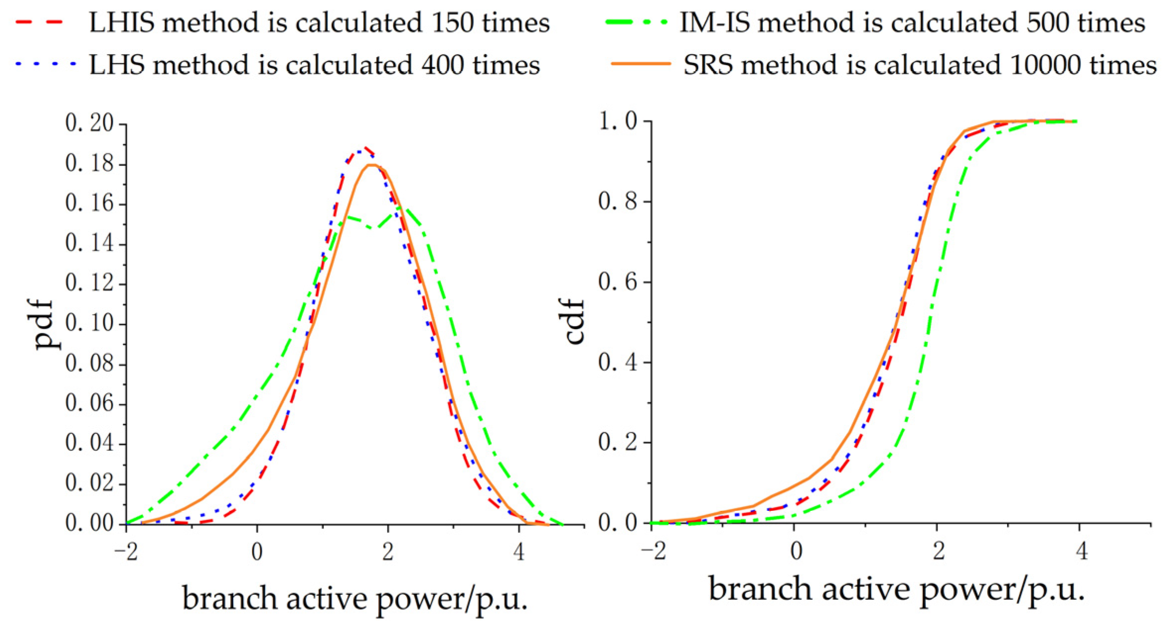
4.1. Verification of Evaluation Methods

In this paper, the accuracy of the evaluation method is measured by the relative error between the expected value and the standard deviation of the results of the probabilistic power flow calculation, and the calculation method is as follows [30]:

$${\epsilon }_{h,\mu }=\left|\frac{{\mu }_{h,\mathrm{acc}}-{\mu }_{h,\mathrm{sim}}}{{\mu }_{h,\mathrm{sim}}}\right|\times 100\%$$

(29)

$${\epsilon }_{h,\sigma }=\left|\frac{{\sigma }_{h,\mathrm{acc}}-{\sigma }_{h,\mathrm{sim}}}{{\sigma }_{h,\mathrm{sim}}}\right|\times 100\%$$

(30)

where ${\mu }_{h,\mathrm{acc}}$ is the expected value, ${\sigma }_{h,\mathrm{acc}}$ is the standard deviation of the calculated results of the probabilistic power flow under a certain sampling scale, ${\mu }_{h,\mathrm{sim}}$ is the expected value, and ${\sigma }_{h,\mathrm{sim}}$ is the standard deviation of the accurate value. In this paper, the result of simple random sampling (SRS) 10,000 times is adopted as the accurate value. h is the physical quantity of the result of the probabilistic power flow calculation and voltage amplitude, u, and line active power, p, are selected as the verification parameters.

Connect a 350 MW wind farm and a 300 MW energy storage system to 15 nodes and use the Latin hypercube important sampling method (LHS) proposed by Huang et al. [7], the improving importance sampling method (IM-IS) proposed by Tómasson et al. [8], and the LHIS method proposed in this paper to perform the probabilistic power flow calculations on the power system. Then, calculate the relative errors of the node voltage, the branch active power expectation, and standard deviation, ${\epsilon }_{u,\mu }$, ${\epsilon }_{u,\sigma }$, ${\epsilon }_{p,\mu }$, ${\epsilon }_{p,\sigma }$, according to Equations (29) and (30). The calculation results are shown in Figure 2. When the relative error of ${\epsilon }_{u,\mu }$ and ${\epsilon }_{p,\mu }$ reaches 0.2%, and the accuracy of ${\epsilon }_{u,\sigma }$ and ${\epsilon }_{p,\sigma }$ reaches 3% of the three calculation methods, the calculation time is calculated, as shown in

Table 3. Calculation time.

	LHIS (s)	LHS (s)	IM-IS (s)
${\epsilon }_{u,\mu }$ (0.2%)	5.002	9.241	9.545
${\epsilon }_{p,\mu }$ (0.2%)	5.091	9.327	10.001
${\epsilon }_{u,\sigma }$ (3%)	6.147	10.202	11.563
${\epsilon }_{p,\sigma }$ (3%)	6.463	10.731	11.799

.

The active power of branch 6–8 is selected as the research object. The probability density function and cumulative distribution function of the calculated results of the LHIS method, the LHS method, and the SRS method are shown in Figure 3.

It can be seen from Figure 2 and Figure 3 that, after the calculation results converge, the relative error of expectation of the LHS and IM-IS calculation results reaches 0.44%, and the relative error of the standard deviation of the LHS and IM-IS calculation results exceeds 4.05%. It can be seen from Table 3 that, when the relative error of the expected value and the relative error of the standard deviation of the calculation result reach 0.2 and 3, respectively, the calculation time of the LHS method and the IM-IS method should be more than 9 s. According to the analysis of Figure 2 and Figure 3 and Table 3, it can be concluded that the LHS method and the IM-IS method still have the problem of poor accuracy of calculation results and a long calculation time.

However, after the calculation results converge, the relative error of expectation of the LHIS method is less than 0.2%, and the relative error of standard deviation of the LHIS method is less than 3%. The calculation result of the LHIS method 150 times is similar to that of the SRS method 10,000 times, while the LHS requires 400 times and the IM-IS requires 500 times. When the evaluation index reaches the allowable accuracy of error, the time that the LHIS method takes is about 5 s, which is nearly 45% shorter than that of the LHS method, and nearly 50% shorter than that of the IM-IS method. It can be concluded that the calculation efficiency of the LHIS method is 40% higher than that of the LHS method and 47% higher than that of the IM-IS method. The calculation accuracy of the LHIS method is 20% higher than that of the LHS method and 33% higher than that of the IM-IS method.

In order to analyze the adaptability of the evaluation methods under different permeability rates, Figure 4 and

Table 4. ${\epsilon }_{u,\mu }$, ${\epsilon }_{u,\sigma }$, ${\epsilon }_{p,\mu }$, and ${\epsilon }_{p,\sigma }$ under different permeability conditions.

	LHIS			LHS			IM-IS
	20%	40%	60%	20%	40%	60%	20%	40%	60%
${\epsilon }_{u,\mu }$ (%)	0.15	0.22	0.26	0.29	0.34	0.38	0.28	0.39	0.41
${\epsilon }_{u,\sigma }$ (%)	2.54	2.78	2.89	2.94	3.23	3.76	2.93	3.51	3.86
${\epsilon }_{p,\mu }$ (%)	0.24	0.29	0.30	0.26	0.32	0.39	0.31	0.39	0.44
${\epsilon }_{p,\sigma }$ (%)	2.76	2.85	2.98	3.01	3.45	3.62	3.31	3.50	4.05

show the error indicators of the three methods under different permeability conditions. The calculation time of the three methods is shown in

Table 5. The calculation time of LHIS, LHS, and IM-IS.

Permeability	LHIS (s)	LHS (s)	IM-IS (s)
20%	5.216	9.321	11.624
40%	5.425	10.012	12.043
60%	5.514	10.424	12.398

.

As can be seen from Figure 4 and Table 4, the relative error of expectation of the LHS and IM-IS calculation results exceeds 0.3% with the increase in permeability, and even the expected relative error of the IM-IS method exceeds 0.4% when the permeability reaches 60%. The relative error of standard deviation of the LHS and IM-IS calculation results exceeds 4% with the increase in permeability. As can be seen from Table 5, when the permeability reaches 60%, the calculation time of LHS and IM-IS exceeds 10 s and 12 s, respectively. According to the analysis of Figure 4 and Table 4 and Table 5, when the power system has high permeability, the LHS and IM-IS methods have obvious lag, the calculation accuracy is poor, and the calculation period is long.

However, with the increase in permeability, the relative error of expectation of the LHIS calculation results does not exceed 0.3%, and the relative error of standard deviation of the LHIS calculation results does not exceed 3%. However, the algorithm still maintains a high precision. The calculation time of the LHIS method also fluctuates in a small range with the increase in permeability, and the calculation time does not exceed 6 s when the permeability reaches 60%. This shows that the LHIS method is universal under the high permeability of the power system and ensures the high precision of the calculation results and a fast calculation time.

4.2. Connecting Wind Farms with Energy Storage Systems at Different Nodes

In order to fully evaluate the influence of wind farms with energy storage systems on the power system at different nodes, this paper chooses to connect a 350 MW wind farm and a 300 MW energy storage system at nodes 1, 2, 13, 15, 16, 18, 21, 22, and 23, and, at the same time, lets the energy storage systems run in charge–discharge strategy 1 and charge–discharge strategy 2, respectively, in order to calculate the $R_{CRI}$ and WSGIEB. The calculation results are shown in Figure 5.

It can be concluded from Figure 5 that the $R_{CRI}$ of Node 1, Node 2, and Node 18 is very high after they are connected to wind farms with energy storage systems. Compared with Table 2, the $R_{CRI}$ exceeds the unacceptable high-risk line and the system reaches the high-risk level after connecting to the wind farms with energy storage systems at Node 2 and Node 18. At the same time, the WSGIEB is negative, therefore, the reliability of the power system is reduced after these three nodes are connected to wind farms with energy storage systems. However, the $R_{CRI}$ of Node 15 is very low and is closest to the negligible low-risk horizontal line, the system operation is in the negligible-risk level, and the WSGIEB is relatively high. Therefore, the reliability of the power system is high after the node is connected to the wind farm with energy storage. Based on the above situation, we can see that it is not suitable to connect wind power at Node 1, Node 2, or Node 18, and the reliability of connecting the wind farm at Node 15 is high.

The reliability of the energy storage systems under charge and discharge strategy 2 is higher than that under charge and discharge strategy 1. This is because, in charging and discharging strategy 2, when the output of the wind turbines cannot reach $P_L(t)·\eta$, the gap will be filled by the output of the conventional power plants first, and the energy storage will be discharged if the sum of the output of the conventional power plants and the wind turbines cannot meet the current power. This discharge strategy can put the energy storage battery in a state of full capacity, or more capacity, for a long time, and, once the power supply is insufficient, there is more energy in the energy storage system to make up for the deficiency. Under charge and discharge strategy 1, the energy storage battery will be discharged for a long time, with relatively low capacity and poor reliability.

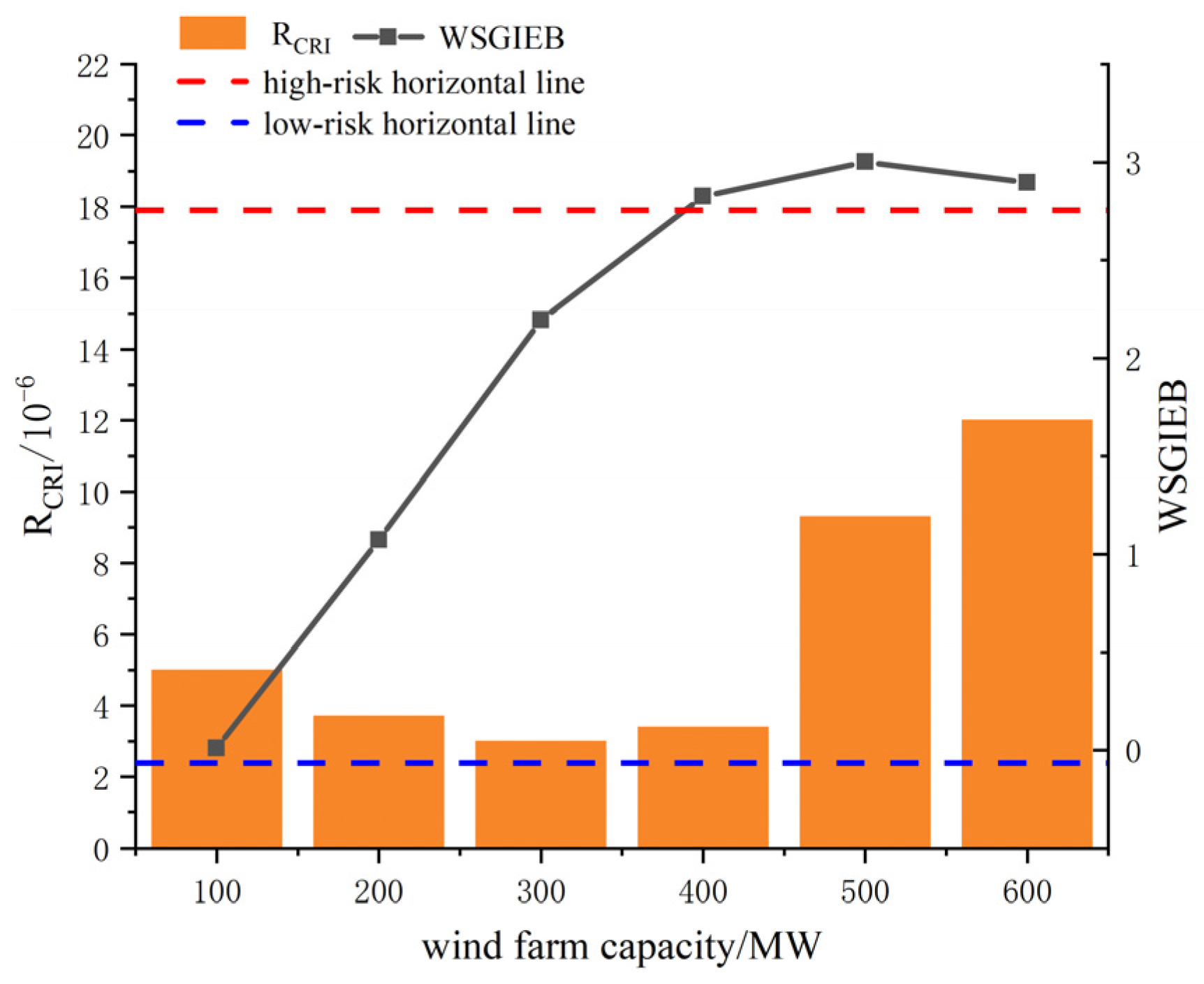
4.3. Connecting Wind Farms of Different Capacities with Energy Storage Systems

According to the analysis results shown in the previous section, the wind farms with energy storage systems are selected to be connected at Node 15, and the energy storage systems are operated under charging and discharging strategy 2, so that the power grid has a higher reliability. The capacity of the energy storage systems is kept constant at 350 MW, and wind power capacities of 100 MW, 200 MW, 300 MW, 400 MW, 500 MW, and 600 MW are connected, respectively. The calculation and evaluation results are shown in Figure 6. With the increase in the connected wind power capacity, the WSGIEB gradually increases, indicating that the increased connected wind power capacity contributes to the reliability of the power system in a certain range; however, when the connected wind power capacity exceeds 500 MW, the WSGIEB decreases, indicating that the newly added wind turbines contribute less and less to the reliability of the power system, resulting in the saturation phenomenon, therefore, further adding wind power capacity will cause a waste of resources.

When the capacity of 15-node-connected wind farms reaches 500 MW, the $R_{CRI}$ increases rapidly. The settlement results of indicators such as $R_{CUT}$, $R_{LINE}$, and $R_V$ are further analyzed, as shown in Figure 7. When the capacity exceeds 500 MW, the $R_V$ and the $R_{LINE}$ increase sharply, which exceeds the unacceptable high-risk line. Through the analysis of Figure 6 and Figure 7, it can be concluded that, when the storage system capacity is 350 MW, it is more appropriate to connect 450 MW of wind power capacity at 15 nodes.

4.4. Connecting Wind Farms with Different Energy Storage Capacities

The capacity of wind farms is kept unchanged at 450 MW, and the energy storage systems capacities of 100 MW, 200 MW, 300 MW, 400 MW, and 500 MW are connected to Node 15, respectively. The calculation results of the evaluation indicators are shown in Figure 8.

With the increase in the energy storage system capacity, the risk of power system failure decreases. In a certain range, the energy storage system capacity increases and the reliability improves. However, when the capacity reaches 400 MW, the value of $R_{CRI}$ is basically unchanged, and the value of WSGIEB will be slightly reduced, mainly because, when the energy storage capacity is too large, the excess output of the wind turbines is completely stored in the energy storage system. Moreover, when the capacity of the energy storage system is increased, the capacity response of the energy storage system reaches saturation, which will not significantly improve the system reliability. When the output of the wind power capacity is kept at 450 MW, the energy storage system capacity of 400 MW is selected in order to optimize the system economy and reliability.

5. Conclusions

In this paper, the LHIS reliability evaluation method was proposed by combining the LHS method and the IS method. Then, the reliability of the power system with wind farms and energy storage systems was evaluated from two aspects of the power system risk and the contribution coefficient to the power system reliability. Through the analysis of the IEEE-RTS79 example, the following conclusions have been obtained:

(1)

Through comparative experiments with the LHIS method, the LHS method, and the IM-IS method, it can be concluded that the calculation efficiency of the LHIS method is 40% higher than that of the LHS method and 47% higher than that of the IM-IS method. The calculation accuracy of the LHIS method is 20% higher than that of the LHS method and 33% higher than that of the IM-IS method.

(2)

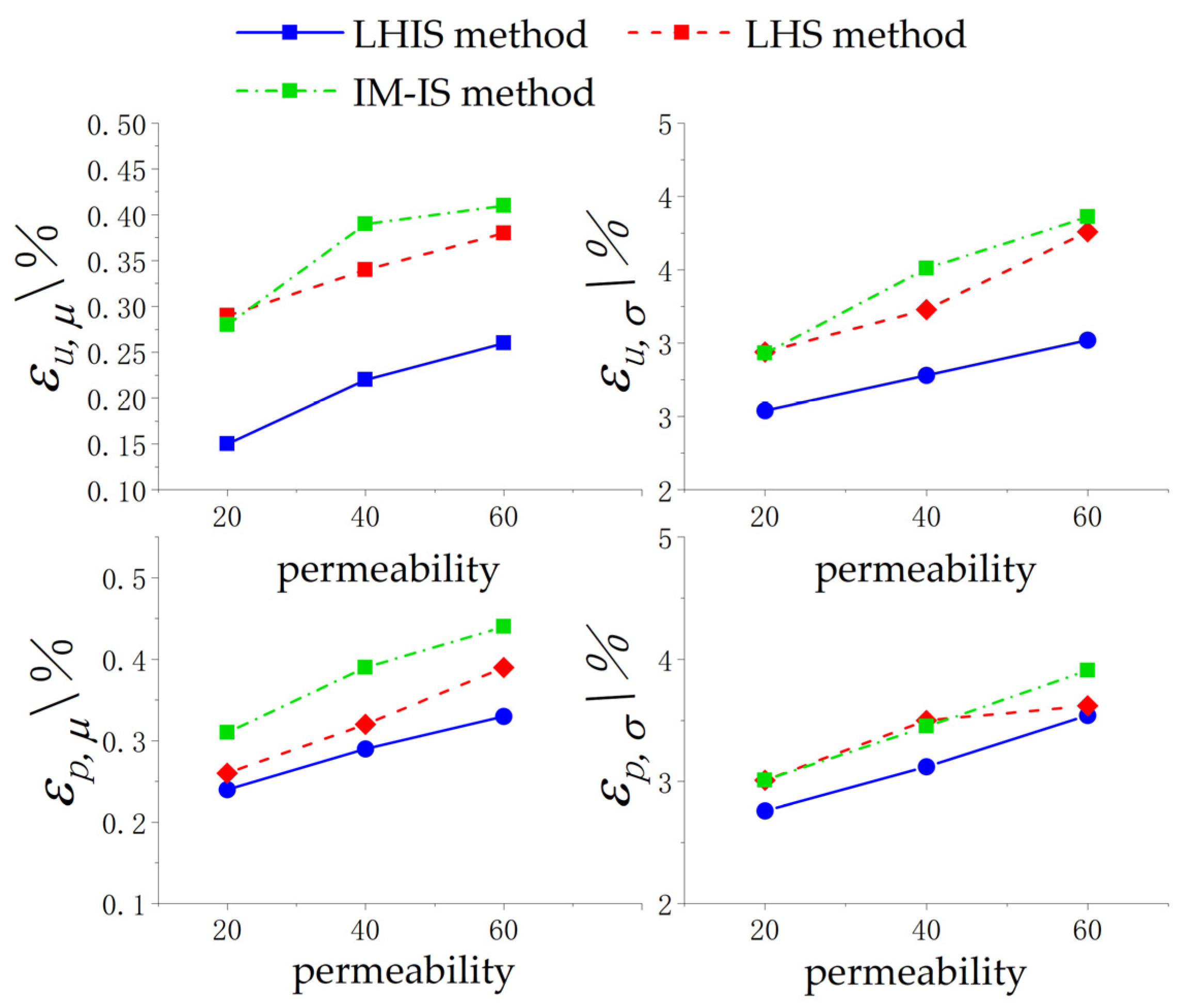
The LHIS method is universal to the reliability analysis of power systems under different permeability conditions. When the permeability reaches 60%, the relative error of expectation does not exceed 0.3%, and the relative error of standard deviation does not exceed 3%. Simultaneously, the calculation time does not exceed 6 s. The LHIS method ensures the high precision of the results and a fast calculation time under high permeability conditions.

(3)

This paper proposed a comprehensive risk indicator to evaluate the operational risk and the wind storage generation interrupted energy benefit (WSGIEB) to evaluate the contribution of the reliability, which solved the problem of a lack of risk analysis of operation state in traditional power system reliability evaluation. Combined with the operation risk division table, the operation of the power system in this state can be more intuitively obtained.

(4)

By analyzing different wind farms with different energy storage system connection strategies, it can be confirmed that the LHIS method can accurately evaluate the reliability of power systems and provide useful references for power system design.

References

1. Yuan, X.M.; Cheng, S.J.; Wen, J.Y. Analysis on the application prospect of energy storage technology in solving large-scale wind power grid connection problems. Power Syst. Autom. 2013, 37, 14–18. [Google Scholar] [CrossRef]
2. Ni, W.; Lv, L.; Xiang, Y.; Liu, J.Y.; Huang, Y.; Wang, P.F. Reliability assessment of integrated energy systems based on Markov Process Monte Carlo method. Power Grid Technol. 2020, 44, 150–158. [Google Scholar] [CrossRef]
3. Gong, L.X.; Liu, T.Q.; He, C.; Nan, L.; Su, X.N.; Hu, X.T. Considering comprehensive gas-electric combined system reliability assessment of demand response. Electr. Power Autom. Equip. 2021, 9, 39–47. [Google Scholar] [CrossRef]
4. Li, Y. Reliability Assessment of Power System with Large-Scale Renewable Energy. Master’s Thesis, Ningxia University, Yinchuan, China, 2020. [Google Scholar]
5. Zhao, Y.; Wang, J.; Geng, L.; Wang, Y.P.; Shuang, Y.J. Extended cross entropy method for non sequential Monte Carlo simulation of power grid reliability. Chin. J. Electr. Eng. 2017, 37, 1963–1974. [Google Scholar] [CrossRef]
6. Jirutitijaroen, P.; Singh, C. Comparison of Simulation Methods for Power System Reliability Indexes and Their Distributions. IEEE Trans. Power Syst. 2008, 23, 486–493. [Google Scholar] [CrossRef]
7. Huang, Y.S.; Chen, S.H.; Chen, Z.; Hu, W.; Huang, Q. Improved probabilistic load flow method based on D-vine Copulas and Latin hypercube sampling in distribution network with multiple wind generators. IET Gener. Transm. Distrib. 2020, 14, 893–899. [Google Scholar] [CrossRef]
8. Tómasson, E.; Söder, L. Generation adequacy analysis of multi-area power systems with a high share of wind power. IEEE Trans. Power Syst. 2018, 33, 3854–3862. [Google Scholar] [CrossRef]
9. Tómasson, E.; Söder, L. Improve important sampling for reliability evaluation of composite power systems. IEEE Trans. Power Syst. 2017, 32, 2426–2434. [Google Scholar] [CrossRef]
10. Cai, J.L.; Xu, Q.S.; Cao, M.J.; Yang, B. A novel importance sampling method of power system reliability assessment considering multi-state units and correlation between wind speed and load. Int. J. Electr. Power Energy Syst. 2019, 109, 217–226. [Google Scholar] [CrossRef]
11. Zhang, W.F.; Che, Y.B.; Liu, Y.S. Improved Latin Hypercube Sampling Method for Reliability Evaluation of Power Systems. Autom. Electr. Power Syst. 2015, 39, 52–57. [Google Scholar] [CrossRef]
12. Oh, U.; Lee, Y.; Choi, J.; Karki, R. Reliability evaluation of power system considering wind generator-s coordinated with multi-energy storage systems. IET Gener. Transm. Distrib. 2020, 14, 786–796. [Google Scholar] [CrossRef]
13. Yuan, M.F.; Zhao, F.Z.; Wang, S.T. Reliability assessment of wind power storage power generation system based on Monte Carlo simulation. Electr. Appl. Energy Effic. Manag. Technol. 2020, 590, 28–34. [Google Scholar] [CrossRef]
14. Jiang, C.; Liu, W.X.; Zhang, J.H.; Yu, Y.; Yu, J.X.; Liu, D.X. Risk assessment of power generation system with battery storage wind farm. J. Sol. Energy 2014, 35, 207–213. [Google Scholar] [CrossRef]
15. Yang, X.Y.; Yang, Y.W.; Liu, Y.Q.; Deng, Z.Q. A reliability assessment approach for electric power systems considering wind power uncertainty. IEEE Access 2020, 8, 12467–12478. [Google Scholar] [CrossRef]
16. Song, T.H.; Li, K.J.; Han, X.Q.; Chen, W.H.; Jia, Y.B.; Wen, F.S. Cooperative operation strategy of energy storage system in multiple application scenarios. Power Syst. Autom. 2021, 45, 43–51. [Google Scholar] [CrossRef]
17. Parvini, Z.; Abbaspour, A.; Fotuhi-Firuzabad, M.; Moeini-Aghtaie, M. Operational reliability studies of power systems in the presence of energy storage systems. IEEE Trans. Power Syst. 2018, 33, 3691–3700. [Google Scholar] [CrossRef]
18. Ponkumar, G.; Jayaprakash, S.; Kanagarathinam, K. Advanced Machine Learning Techniques for Accurate Very-Short-Term Wind Power Forecasting in Wind Energy Systems Using Historical Data Analysis. Energies 2023, 16, 5459. [Google Scholar] [CrossRef]
19. Pan, C.Q.; Wang, C.; Zhao, Z.Y.; Wang, J.; Bie, Z. A copula function based Monte Carlo simulation method of multivariate wind speed and PV power spatio-temporal series. Energy Procedia 2019, 15, 213–218. [Google Scholar] [CrossRef]
20. Huang, D.; Yang, X.; Gao, L.; Zang, C.; Chen, H.Y. Multi-objective cooperative game interval economic scheduling considering wind power and energy storage connected to power grid. Control Theory Appl. 2021, 38, 1061–1070. [Google Scholar] [CrossRef]
21. Shezan, S.A.; Kamwa, I.; Ishraque, M.F.; Muyeen, S.M.; Hasan, K.N.; Saidur, R.; Rizvi, S.M.; Shafiullah, M.; Al-Sulaiman, F.A. Evaluation of Different Optimization Techniques and Control Strategies of Hybrid Microgrid. Energies 2023, 16, 1792. [Google Scholar] [CrossRef]
22. Cai, J.L.; Hao, L.L.; Zhang, K.Q. Non-parametric importance stratified sampling method for Reliability evaluation of power systems with renewable energy. Autom. Electr. Power Syst. 2012, 46, 104–115. [Google Scholar] [CrossRef]
23. Zhao, Y.; Liu, Y.; Ren, H.; Cheng, X.Y.; Xie, K.G. Optimal f-divergence importance sampling method for reliability evaluation of large power grids. J. Electr. Eng. China 2022, 42, 5067–5079. [Google Scholar] [CrossRef]
24. Li, H.; Hu, X.D.; Xuan, W.B. Important sampling effect increment method for reliability evaluation of power systems. J. Power Syst. Autom. 2020, 32, 117–124. [Google Scholar] [CrossRef]
25. Jiang, C.; Wang, S.; Wang, B.Q.; Zhang, J.H.; Zhao, T.Y. Probabilistic reliability assessment of power systems with wind power based on Latin Hypercube sampling. Trans. China Electrotech. Soc. 2016, 31, 193–206. [Google Scholar] [CrossRef]
26. Osama, A.A.; Chung, C.Y. A hybrid framework for short-term risk assessment of wind-integrated composite power systems. IEEE Trans. Power Syst. 2019, 34, 2334–2344. [Google Scholar] [CrossRef]
27. Li, X.; Zhang, X.; Wu, L.; Lu, P.; Zhang, S.H. Transmission line overload risk assessment for power systems with wind and load-power generation correlation. IEEE Trans. Smart Grid 2015, 6, 1233–1242. [Google Scholar] [CrossRef]
28. Ma, Y.F.; Yang, X.K.; Wang, Z.J.; Dong, L.; Zhao, S.Q.; Cai, Y.Q. Operation risk assessment of large-scale wind power grid connected power system based on value-at-risk. Power Grid Technol. 2021, 45, 849–855. [Google Scholar] [CrossRef]
29. Ma, Y.F.; Luo, Z.R.; Zhao, S.Q.; Wang, Z.J.; Xie, J.R.; Zeng, S.M. Risk assessment of wind power system based on improved Monte Carlo mixed sampling. Power Syst. Prot. Control 2022, 50, 75–83. [Google Scholar] [CrossRef]
30. Zhang, Z.H.; Li, Y.T.; He, L.Z.; Yao, F. Application of monte carlo method in static safety risk assessment of power system. Electr. Meas. Instrum. 2015, 52, 106–111. [Google Scholar] [CrossRef]
31. Shang, H.Y.; Liu, T.Q.; Bu, T.; He, C.; Yin, Y.; Ding, L.J. Risk assessment of high proportion new energy grid connected systems based on the ALARP criterion. Power Autom. Equip. 2021, 41, 196–203. [Google Scholar] [CrossRef]
32. Gao, F.Y.; Yuan, C.; Li, Z.J.; Qi, X.D.; Zhuang, S.X. Probabilistic power flow calculation based on approximate Bayesian calculation combined with Markov chain Monte Carlo. J. Sol. Energy 2021, 42, 265–272. [Google Scholar] [CrossRef]
Figure 1. Evaluation flow chart.
Energies 16 06427 g001
Figure 2. ε u , μ , ε u , σ , ε p , μ , and ε p , σ relative error curves.
Energies 16 06427 g002
Figure 3. Active power probability distribution curve.
Energies 16 06427 g003
Figure 4. ε u , μ , ε u , σ , ε p , μ , and ε p , σ relative error curves under different permeability conditions.
Energies 16 06427 g004
Figure 5. Evaluation indexes of grid connection of wind farms with energy storage systems at different nodes.
Energies 16 06427 g005
Figure 6. Evaluation indexes of wind farms with different capacities connected with energy storage.
Energies 16 06427 g006
Figure 7. Calculation results of R C U T , R L I N E , and R V .
Energies 16 06427 g007
Figure 8. Evaluation indicators of wind farms with different energy storage capacities.
Energies 16 06427 g008